DLCV 01A · Training Deep Vision Models in Practice
Needs: DLCV 01 · Deep Learning for Image Processing and Computer Vision
Navigate: this page and this track: Navigate: this page and this track
On this page
- What you’ll learn1 min
- The big picture2 min
- A training checklist2 min
- The data pipeline5 min
- Initialization and normalization in practice2 min
- Choosing the learning rate7 min
- Batch size and gradient accumulation2 min
- Regularization in practice3 min
- Mixed precision and loss scaling1 min
- Transfer learning and fine-tuning strategies2 min
- Debugging a training run5 min
- Reproducibility and fair experiments3 min
- Modern view3 min
- Key takeaways1 min
- Exercises3 min
- Supplementary notes
- Paper guides
- References
Deep Learning for Computer Vision
What you’ll learn
- Build a training workflow that catches cheap mistakes before expensive runs.
- Prevent data leakage and keep image augmentations consistent with labels.
- Choose learning rates, schedules, batch sizes and gradient accumulation settings.
- Apply regularization, mixed precision and pretrained-model fine-tuning.
- Debug losses and gradients, then compare models with controlled budgets and multiple seeds.
The big picture
You already know how convolutional and transformer networks for images are built (DLCV 01). This chapter is about the other half of the job: getting one to train well, quickly, and knowing whether a result is real.
Why spend a chapter on this? Because the recipe often matters as much as the architecture. He et al. combined training refinements, such as learning-rate warmup and cosine decay, with small changes to the network and raised the ImageNet top-1 accuracy of ResNet-50 from 75.3% to 79.29% [1]; DLCV 02 describes a similar result. And training failures are often silent: a network with a bug in its data pipeline usually still trains, just worse, so nothing crashes to warn you [2]. The habits in this chapter are how practitioners catch those bugs early.
The theory behind most tools is already covered elsewhere on this site, and this chapter links to it instead of repeating it:
| Topic | Covered in depth in |
|---|---|
| Floating point, gradient checks, a debugging order for NaN values | ML 01C |
| SGD, momentum, Adam, AdamW, initialization, normalization layers, gradient clipping, basic schedules | ML 02 |
| Baselines, splits and leakage, significance tests, reproducibility, latency and deployment | ML 11 |
| How batch normalization works; knowledge distillation | DLCV 01 notes |
| Classification recipes: augmentation, loss and optimizer choices, transfer learning, calibration | DLCV 02 |
What this chapter adds is the workflow: the order in which to do things, the quick tests that catch mistakes, and the defaults that work for most vision models.
A training checklist
Plain version. Before a large run, verify that a small model can fit one batch. Change one factor at a time.
The list below is the whole chapter in one place. Each item links to the section that explains it.
- Fix the evaluation first. Define the split unit, the metric and a simple baseline before training anything (data pipeline; ML 11).
- Look at the data. Plot a batch after the full input pipeline (decoding, resizing, augmentation, normalization), with its labels drawn on top. This catches most pipeline bugs in a minute.
- Start from known-good defaults. A standard architecture, He initialization, a pretrained backbone if one exists, AdamW or SGD with momentum (initialization).
- Overfit one batch. The training loss on a single fixed batch must go to almost zero (debugging).
- Find the learning rate with a short range test, then pick a schedule with warmup and a decay (learning rate).
- Set the batch size from memory, and scale the learning rate with it (batch size).
- Train the full model, log everything (losses, metrics, learning rate, gradient norms), and keep the best checkpoint by validation score.
- Regularize only when you see overfitting, one tool at a time (regularization).
- Speed up with mixed precision once the run is correct (mixed precision).
- Compare fairly: same budget, same data, several seeds, one change per ablation; open the test set once at the end (fair experiments).
The running example
To show each step with real numbers, the snippets train a small multilayer perceptron (MLP) written in NumPy: 64 inputs, one hidden layer of 32 ReLU units and 10 outputs, trained with SGD and momentum on scikit-learn’s handwritten digits [3]. It is not a deep vision model, but every training decision in this chapter applies to it, and each run takes well under a second on a CPU. All numbers called “our toy runs” below come from this code; the figure script scripts/figures/dl_01a_training_practice.py reproduces them.
The code below defines it once: data loading with a stratified split, normalization with training-split statistics, a two-layer network with He initialization, backpropagation, and a training loop that accepts any learning-rate schedule. The loop also keeps an exponential moving average of the weights, which the EMA section uses. Later snippets reuse these functions, so run this block first.
Code · Python · 65 lines
import numpy as np
from sklearn.datasets import load_digits
from sklearn.model_selection import train_test_split

X, y = load_digits(return_X_y=True)                     # 1,797 images of 8x8 pixels, 10 classes
X_tmp, X_te, y_tmp, y_te = train_test_split(X, y, test_size=0.3, stratify=y, random_state=0)
X_tr, X_va, y_tr, y_va = train_test_split(X_tmp, y_tmp, test_size=0.25, stratify=y_tmp, random_state=0)
mu, sd = X_tr.mean(0), X_tr.std(0) + 1e-8               # statistics of the TRAINING split only
X_tr, X_va, X_te = [(a - mu) / sd for a in (X_tr, X_va, X_te)]

def init(seed, sizes=(64, 32, 10)):                     # He initialization for ReLU layers
    rng = np.random.default_rng(seed)
    return [[rng.normal(0, np.sqrt(2 / m), (m, n)), np.zeros(n)]
            for m, n in zip(sizes[:-1], sizes[1:])]

def forward(P, X):
    h = [X]
    for i, (W, b) in enumerate(P):
        z = h[-1] @ W + b
        h.append(np.maximum(z, 0) if i < len(P) - 1 else z)   # ReLU; the last layer gives logits
    return h

def loss_and_grads(P, X, y):
    h = forward(P, X)
    z = h[-1] - h[-1].max(1, keepdims=True)             # stable log-softmax
    logp = z - np.log(np.exp(z).sum(1, keepdims=True))
    loss = -logp[np.arange(len(y)), y].mean()           # cross-entropy
    d = np.exp(logp)                                    # softmax probabilities
    d[np.arange(len(y)), y] -= 1
    d /= len(y)                                         # dLoss/dlogits
    grads = []
    for i in reversed(range(len(P))):
        grads.insert(0, [h[i].T @ d, d.sum(0)])
        if i:
            d = (d @ P[i][0].T) * (h[i] > 0)            # back through the ReLU
    return loss, grads

def evaluate(P, X, y):
    z = forward(P, X)[-1]
    z = z - z.max(1, keepdims=True)
    logp = z - np.log(np.exp(z).sum(1, keepdims=True))
    return -logp[np.arange(len(y)), y].mean(), (z.argmax(1) == y).mean()

def train(schedule, peak, epochs=15, bs=16, momentum=0.9, seed=0, ema_decay=0.99):
    P = init(seed)
    V = [[np.zeros_like(W), np.zeros_like(b)] for W, b in P]   # momentum buffers
    E = [[W.copy(), b.copy()] for W, b in P]                    # EMA copy of the weights
    rng = np.random.default_rng(seed + 1000)            # data order depends on the seed too
    T, t, log = epochs * int(np.ceil(len(y_tr) / bs)), 0, []
    for _ in range(epochs):
        order = rng.permutation(len(y_tr))
        for i in range(0, len(y_tr), bs):
            idx = order[i:i + bs]
            _, G = loss_and_grads(P, X_tr[idx], y_tr[idx])
            lr = schedule(t, T, peak)
            t += 1
            for (W, b), (gW, gb), v, e in zip(P, G, V, E):   # SGD with momentum, in place
                v[0] = momentum * v[0] + gW
                v[1] = momentum * v[1] + gb
                W -= lr * v[0]
                b -= lr * v[1]
                e[0] += (1 - ema_decay) * (W - e[0])    # e <- decay * e + (1 - decay) * w
                e[1] += (1 - ema_decay) * (b - e[1])
        log.append(evaluate(P, X_tr, y_tr) + evaluate(P, X_va, y_va))
    return P, np.array(log), E   # log columns: train loss, train acc, val loss, val acc
The split is 942 training, 315 validation and 540 test images; the test images are not touched in this chapter.
The data pipeline
Plain version. Inspect the tensors produced by the full data pipeline. Their values and labels determine both learning and evaluation validity.
Splits, leakage and the test set
The test set must be new in the same way deployment data will be new. Split by the unit that will be new (patient, video, camera, site or time period), deduplicate before splitting, fit every preprocessing step on the training split only, and use the validation set for all decisions so that the test set is opened once. ML 11 covers the forms leakage takes and how to measure uncertainty; this chapter assumes those rules.
Normalization statistics
Networks train best when each input channel has a mean near zero and a spread near one. The standard step is
where is a pixel value in channel (for example red, green or blue), and are the mean and standard deviation of channel , and is the value the network sees. Two practical rules follow.
- Training from scratch: compute and on the training split only, store them with the model, and apply the same stored values at validation, test and deployment time. The running example does exactly this, per pixel rather than per channel.
- Fine-tuning a pretrained model: use the statistics the model was pretrained with, not those of your new dataset. The first layer’s filters were learned for inputs on that scale.
The most common bug here is a mismatch: images scaled to in training but raw – values in deployment, or RGB in one place and BGR in another. Both still produce predictions, just bad ones.
Class imbalance
Plain version. Class imbalance can hide rare-class failures behind high overall accuracy. Adjust sampling, loss weights or classifier initialization.
Buda et al. compared remedies for convolutional networks on benchmarks of increasing difficulty [4]. In their experiments oversampling the rare classes was the dominant method in almost all scenarios, it worked best when it removed the imbalance completely, and, unlike for some classical models, it did not cause the networks to overfit; they also recommend thresholding to compensate for the class priors when overall accuracy is what matters [4]. The three levers look like this:
Code · Python · 17 lines
import numpy as np

counts = np.array([900, 80, 20])                        # training images per class
labels = np.repeat([0, 1, 2], counts)

w = counts.sum() / (len(counts) * counts)               # option 1: weight the loss
print("loss weight per class:", np.round(w, 2))

p = 1.0 / counts[labels]                                # option 2: oversample rare classes
p /= p.sum()
rng = np.random.default_rng(0)
drawn = labels[rng.choice(len(labels), size=3000, p=p)]
print("class share in 3,000 sampled examples:", np.round(np.bincount(drawn) / 3000, 3))

prior = counts / counts.sum()                           # option 3: start the output bias at the prior
b0 = np.log(prior)
print("initial softmax output:", np.round(np.exp(b0) / np.exp(b0).sum(), 3))
Output
loss weight per class: [ 0.37  4.17 16.67]
class share in 3,000 sampled examples: [0.33  0.338 0.332]
initial softmax output: [0.9  0.08 0.02]
Option 1 multiplies each example’s loss by , where is the number of training examples, the number of classes and the count of class . Option 2 draws each example with probability proportional to , so every class appears equally often. Option 3 sets the output biases to , so the untrained network already predicts the class frequencies; Lin et al. use the same idea in dense detection, starting every location at a foreground probability of about 0.01 [5] (see the focal loss in DLCV 03). Whatever you choose, report per-class metrics (DLCV 02).
Augmentation as a regularizer
Plain version. Augmentation shows the network a slightly different version of each image every time, so it cannot memorize pixels and must learn what stays the same. The golden rule: a transformation is allowed only if the correct label of the new image is known.
That rule decides the augmentation for each task:
| Task | Usually safe | Needs care or is wrong |
|---|---|---|
| Classification of photos | random crops and rescaling, horizontal flips, color jitter, mild blur | vertical flips for upright scenes; flips for text, digits and left/right-sensitive classes |
| Detection | flips, crops, scaling, color jitter, applied to the image and the boxes | crops that cut objects: clip the box and drop it if too little is left |
| Segmentation | the same geometry applied to the image and the mask | interpolating the mask: resize labels with nearest neighbor, never bilinear |
| Keypoints and pose | geometry applied to the image and the points | a horizontal flip must also swap left and right keypoint labels (DLCV 05) |
| Restoration and low-level vision | flips, 90° rotations, crops applied identically to input and target | color or blur augmentation that changes the target itself |
| Medical and remote sensing | rotations where orientation carries no meaning | intensity changes that alter diagnostic values |
For dense tasks the key word is consistency: every geometric change applied to the pixels must be applied to the labels in the same coordinates. The snippet flips and crops a photo of coins together with a segmentation mask and a bounding box for one coin, then checks that the transformed box equals the box of the transformed mask:
Code · Python · 26 lines
import numpy as np
from scipy import ndimage
from skimage import data, filters, measure, segmentation

img = data.coins()                                      # 303 x 384 grayscale photo
fg = segmentation.clear_border(img > filters.threshold_otsu(img))
lab = measure.label(ndimage.binary_fill_holes(fg))
coin = max(measure.regionprops(lab), key=lambda r: r.area)
mask = lab == coin.label                                # segmentation target for one coin
box = tuple(int(v) for v in coin.bbox)                  # detection target (y0, x0, y1, x1)
H, W = img.shape

def hflip(img, mask, box):
    y0, x0, y1, x1 = box
    return img[:, ::-1], mask[:, ::-1], (y0, W - x1, y1, W - x0)

def crop(img, mask, box, top, left, h, w):
    y0, x0, y1, x1 = box                                # shift, then clip to the crop
    new = (max(y0 - top, 0), max(x0 - left, 0), min(y1 - top, h), min(x1 - left, w))
    return img[top:top + h, left:left + w], mask[top:top + h, left:left + w], new

i2, m2, b2 = crop(*hflip(img, mask, box), top=90, left=0, h=180, w=240)
r, c = np.nonzero(m2)
print("original box:               ", box)
print("box after flip + crop:      ", b2)
print("box of the transformed mask:", (int(r.min()), int(c.min()), int(r.max()) + 1, int(c.max()) + 1))
Output
original box:                (156, 315, 218, 380)
box after flip + crop:       (66, 4, 128, 69)
box of the transformed mask: (66, 4, 128, 69)
Under a horizontal flip of an image of width , a box with columns to moves to columns to : the edges swap roles. Flipping the image but not its labels gives the network contradictory targets (Figure 1, right). Karpathy lists exactly this kind of mistake, flipping images without flipping their labels, among the bugs that make a network train silently worse instead of failing [2]. In practice, use a library that transforms images together with their masks and boxes, such as Albumentations [6], and still verify it once with a check like the one above.
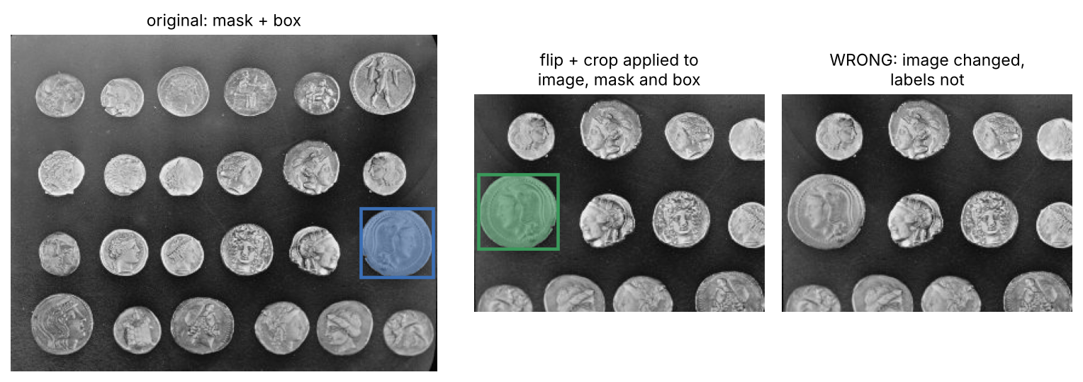
How strong? Augmentation strength is a hyperparameter: tune it on the validation set, and expect a strongly augmented model to show a higher training loss than validation loss. Shorten and Khoshgoftaar survey the families of image augmentation [7]; DLCV 02 shows the mixing augmentations of modern classification recipes.
Initialization and normalization in practice
Plain version. A good start keeps the signal at a sensible size through every layer, so the first steps of training are spent learning instead of recovering from a bad scale. For standard architectures, the defaults below are well tested; use them unless you have a reason not to.
- Weights. Use He initialization for layers followed by ReLU-like activations: draw weights with variance , where is the number of inputs to a unit, which keeps the activation variance roughly constant across layers [8]. Biases start at zero. ML 02 derives this.
- Residual blocks. Initialize the scale of the last batch-normalization layer in each residual branch to zero. Each block then starts as the identity, the signal travels through the shortcuts, and early training is easier; Goyal et al. found that this helped all their models and especially large-batch training [9], and He et al. include it in their bag of tricks [1].
- Output layer. Initialize the classifier bias at the log class prior when classes are imbalanced (option 3 above).
- Pretrained weights. When a pretrained backbone exists for your input type, start from it. A new head is the only part initialized from scratch.
Normalization layers in practice. Batch normalization (BN) [10] standardizes each channel with the mean and variance of the current mini-batch, then keeps running averages for inference (DLCV 01 note). Two habits avoid most BN problems:
- Switch modes. Training mode uses batch statistics and updates the running averages; evaluation mode uses the stored averages. Forgetting to switch to evaluation mode at test time is a classic bug.
- Watch the per-device batch size. BN statistics are computed over the examples on one device. With only one or two images per device, as is common in detection and segmentation, the statistics become noisy. Group Normalization, which normalizes groups of channels within each example, does not depend on the batch size and stays accurate where BN degrades; Wu and He also describe the common detection practice of freezing a pretrained backbone’s BN, using its stored statistics as a fixed linear layer [11].
Transformers use a normalization computed within each example, which does not depend on the batch; ML 02 compares the normalization layers.
Choosing the learning rate
Plain version. The learning rate is the size of each step downhill. Too small and training crawls; too large and the loss jumps around or explodes. The best rate also changes during training: larger steps help early, smaller steps help at the end.
Bengio wrote that the learning rate is often the single most important hyperparameter [12]. The procedure here: measure the usable range once, then let a schedule move through it.
The learning-rate range test
Plain version. Run training once while raising the learning rate a little at every step, and watch the loss. Where the loss stops falling and starts to climb, the rate has become too large.
Smith introduced this learning-rate range test together with cyclical learning rates: train for a short time while increasing the rate between a low and a high value, and read off the range in which the network still learns [13]. In his later guidance, the rate where the loss is lowest (or the accuracy highest) is the largest usable value, a suitable maximum for a schedule that ramps up and down, while a constant learning rate must be smaller or the network will not begin to converge; for a single-cycle schedule he suggests a minimum 10 to 20 times below the maximum [14].
Smith reads the curve from the validation loss or accuracy; our version uses the training loss of each batch, which costs nothing extra. It increases the rate exponentially from to over at most 200 steps, so that every decade gets equal time, and smooths the noisy batch loss with an exponential moving average:
where is the loss of the batch at step , the running average (starting from ), the smoothing factor, and the bias-corrected average that is plotted; the correction removes the pull toward the zero starting value. The test stops when the smoothed loss exceeds four times its minimum. The code below reuses init and loss_and_grads from the running example.
Code · Python · 26 lines
def lr_range_test(lo=1e-4, hi=10.0, steps=200, bs=16, momentum=0.9, seed=0):
    P = init(seed)
    V = [[np.zeros_like(W), np.zeros_like(b)] for W, b in P]
    rng = np.random.default_rng(seed)
    lrs, smooth, avg = [], [], 0.0
    for t in range(steps):
        lr = lo * (hi / lo) ** (t / (steps - 1))        # exponential sweep
        idx = rng.choice(len(y_tr), bs, replace=False)
        loss, G = loss_and_grads(P, X_tr[idx], y_tr[idx])
        avg = 0.9 * avg + 0.1 * loss                    # smooth the noisy batch loss
        lrs.append(lr)
        smooth.append(avg / (1 - 0.9 ** (t + 1)))       # bias-corrected average
        if not np.isfinite(loss) or smooth[-1] > 4 * min(smooth):
            break                                       # the loss has blown up: stop
        for (W, b), (gW, gb), v in zip(P, G, V):
            v[0] = momentum * v[0] + gW
            v[1] = momentum * v[1] + gb
            W -= lr * v[0]
            b -= lr * v[1]
    return np.array(lrs), np.array(smooth)

lrs, smooth = lr_range_test()
best = lrs[smooth.argmin()]
print(f"lowest smoothed loss {smooth.min():.3f} at lr {best:.3f}; stopped at lr {lrs[-1]:.3f}")
print(f"suggested peak for a one-cycle or warmup schedule: about {best:.2f}")
print(f"suggested constant learning rate: about {best / 10:.3f}")
Output
lowest smoothed loss 0.270 at lr 0.138; stopped at lr 0.392
suggested peak for a one-cycle or warmup schedule: about 0.14
suggested constant learning rate: about 0.014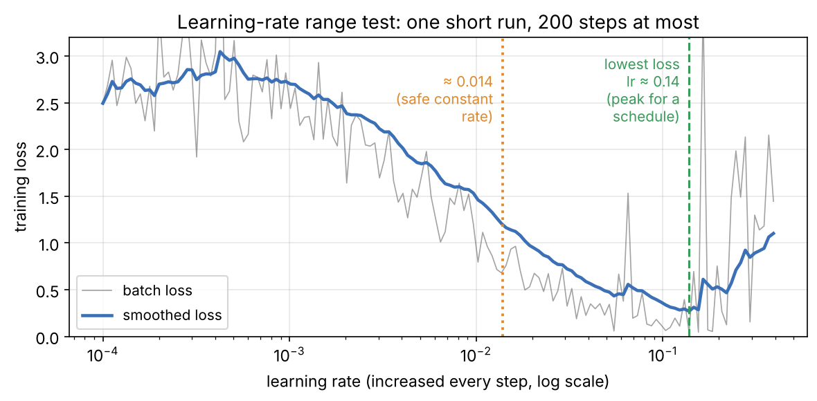
Read Figure 2 from left to right: too small to change anything, then the useful range where the loss falls steeply, then steps that are too large. The code takes a tenth of the minimum as the constant rate; that factor is our rule of thumb, not a value from [14]. A range test costs a few hundred steps, so rerun it whenever you change the model, batch size, optimizer or weight decay. Treat the result as a range, not an exact value: the curve is noisy and depends on the seed.
Warmup
Plain version. Start with a small learning rate and raise it to the target over the first few hundred or thousand steps. At the start, the weights are random and the optimizer’s running statistics are empty, so a full-size step can throw the model into a bad region it never leaves.
With a linear warmup over steps, the rate at step is
where is the target rate reached at the end of warmup. Goyal et al. showed why the shape matters: in large-batch ImageNet training, a constant low rate for the first epochs followed by a jump to the target made the training error spike, while a gradual ramp avoided that spike [9]. Warmup matters most for large batches, large learning rates, adaptive optimizers and Transformers, and it is cheap insurance in fine-tuning. Goyal et al. report that even a constant low-rate warmup was particularly helpful when prototyping detection and segmentation models that fine-tune pretrained layers together with new ones [9]. Our toy warms up over the first 5% of the steps.
Schedules: step, cosine and one-cycle
Plain version. After warmup, the rate should fall. How it falls matters less than that it falls: large steps explore, small steps at the end settle into a good region.
ML 02 introduces step decay, cosine annealing and warmup; this section adds one-cycle and compares all of them on one problem. Write for the current step, for the total number of steps and for the largest rate. The four schedules in Figure 3 are:
- Constant: . Simple, but the final steps are as large as the first ones.
- Step decay: multiply the rate by a factor (often 0.1) at fixed milestones, for example at 50% and 75% of training. The classic choice for CNNs trained with SGD.
- Warmup + cosine: after warmup steps, with progress running from 0 to 1, so the rate glides from to zero. The cosine shape comes from SGDR, which also restarted it periodically [15]; He et al. adopted the plain cosine decay for ImageNet classification, where it improved accuracy over their step-decay baseline [1].
- One-cycle: a single long rise from a low rate to , then a fall to a value far below the starting rate. Smith and Topin used this “1cycle” policy with a large maximum rate to train some networks much faster than with standard schedules, which they called super-convergence [16]. Our version follows the defaults of PyTorch’s
OneCycleLR: a cosine-shaped rise over the first 30% of steps from , then a cosine fall to times below the start [17]. That implementation also lowers the momentum while the rate rises, as Smith recommends [14]; our toy keeps momentum fixed.
Code · Python · 26 lines
import numpy as np

def constant(t, T, peak):
    return peak

def step_decay(t, T, peak, milestones=(0.5, 0.75), factor=0.1):
    return peak * factor ** sum(t >= m * T for m in milestones)

def warmup_cosine(t, T, peak, warmup=0.05):
    W = max(1, int(warmup * T))
    if t < W:
        return peak * (t + 1) / W                       # linear warmup
    q = (t - W) / max(1, T - W)                         # progress after warmup, 0 -> 1
    return 0.5 * peak * (1 + np.cos(np.pi * q))         # cosine decay to 0

def one_cycle(t, T, peak, pct=0.3, div=25, final_div=1e4):
    up, lo = max(1, int(pct * T)), peak / div
    if t < up:                                          # rise from peak/div to peak
        return lo + (peak - lo) * 0.5 * (1 - np.cos(np.pi * t / up))
    q = (t - up) / max(1, T - up)                       # fall far below the start
    end = lo / final_div
    return end + (peak - end) * 0.5 * (1 + np.cos(np.pi * q))

T = 900
for f in (constant, step_decay, warmup_cosine, one_cycle):
    print(f"{f.__name__:13s}", [f"{f(t, T, 0.1):.2g}" for t in (0, 20, 270, 450, 700, 899)])
Output
constant      ['0.1', '0.1', '0.1', '0.1', '0.1', '0.1']
step_decay    ['0.1', '0.1', '0.1', '0.01', '0.001', '0.001']
warmup_cosine ['0.0022', '0.047', '0.084', '0.054', '0.013', '3.4e-07']
one_cycle     ['0.004', '0.0053', '0.1', '0.081', '0.023', '1e-06']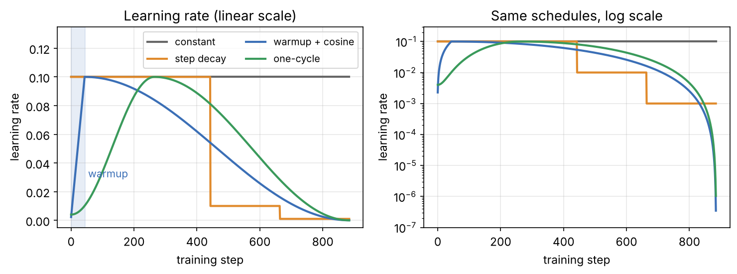
Optional: Cosine annealing with warm restarts (in the Supplementary notes). The SGDR formula with restart periods, and when restarts are useful.
What the schedules do on the toy
The loop below trains the running example once with each schedule at a peak of 0.1, and once more with a constant rate of 0.01. It uses train from the running example and the schedule functions just above.
Code · Python · 5 lines
for f in (constant, step_decay, warmup_cosine, one_cycle):
    _, log, _ = train(f, peak=0.1)
    print(f"{f.__name__:13s} peak 0.1   final train loss {log[-1, 0]:8.3f}   val acc {log[-1, 3]:.3f}")
_, log, _ = train(constant, peak=0.01)
print(f"{'constant':13s} peak 0.01  final train loss {log[-1, 0]:8.3f}   val acc {log[-1, 3]:.3f}")
Output
constant      peak 0.1   final train loss  995.468   val acc 0.917
step_decay    peak 0.1   final train loss    0.000   val acc 0.940
warmup_cosine peak 0.1   final train loss    0.000   val acc 0.971
one_cycle     peak 0.1   final train loss    0.000   val acc 0.956
constant      peak 0.01  final train loss    0.021   val acc 0.959
Figure 4 shows the runs epoch by epoch. Three lessons come out of this toy, and they match the advice above:
- A peak near the edge needs a schedule. At a constant 0.1, close to the range-test minimum, the loss explodes and validation accuracy swings between 81% and 92%. The same peak is fine inside a schedule that ramps up and decays (warmup + cosine reached 97.1%, one-cycle 95.6% in this run).
- Decay rescues, but late. Step decay spends half of training at the unstable rate; once the rate drops, during epoch 8, the loss recovers and validation accuracy reaches 94.0%.
- A constant rate can work if it is small. At 0.01, a tenth of the peak as the range test suggested, the constant schedule trains smoothly (95.9%), just less far in the same budget: its training loss is still 0.021.
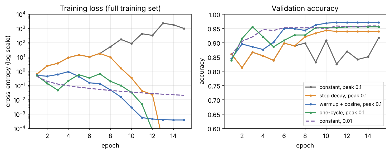
Do not read the ranking between cosine and one-cycle into this figure: it is one seed, and the seed study below shows that their order flips from seed to seed. The robust lesson is the first one.
Which schedule to pick. Warmup followed by cosine decay is a safe default; step decay is fine when reproducing an older paper; one-cycle suits short budgets; a constant rate with a short final decay helps when the training length is not known in advance (Modern view). Schedules are defined in steps, so recompute when the epochs, batch size or dataset size change.
Batch size and gradient accumulation
Plain version. A bigger batch gives a less noisy gradient, so each step can be bigger. If you double the batch, you can usually double the learning rate, up to a point. (ML 02 defines batches, iterations and epochs.)
Goyal et al. trained ResNet-50 [18] on ImageNet [19] with mini-batches of up to 8,192 images without losing accuracy, using two rules [9]:
- Linear scaling rule: when the mini-batch size is multiplied by , multiply the learning rate by and keep the other hyperparameters, such as weight decay, unchanged. He et al. state the same rule in the form for a ResNet-50 trained with SGD at batch size [1].
- Gradual warmup: ramp the rate from the small-batch value to the scaled value over the first 5 epochs.
The rule is an approximation. It assumes the gradient changes little over the small steps that one big step replaces, which fails early in training (hence warmup) and beyond some batch size; in their ImageNet experiments that limit was around 8,000 images [9]. For adaptive optimizers the relationship is less simple, so re-run the range test after a large change in batch size.
Optional: Accurate, Large Minibatch SGD (Goyal et al.) (in the Paper guides). Where the scaling rule comes from, how to read their warmup comparison, and the implementation pitfalls they list.
Gradient accumulation. When the batch you want does not fit in memory, run several smaller micro-batches, add up their gradients, and take one optimizer step. With a loss that is a mean over examples and micro-batches of equal size,
where is the mean loss over all examples, the mean loss over micro-batch of examples, and the parameters. The snippet checks this on the toy (it reuses init and loss_and_grads from the running example):
Code · Python · 13 lines
P = init(0)
xb, yb = X_tr[:32], y_tr[:32]
_, full = loss_and_grads(P, xb, yb)                     # one batch of 32

acc = [[np.zeros_like(W), np.zeros_like(b)] for W, b in P]
k = 4                                                   # 4 micro-batches of 8
for j in range(k):
    _, G = loss_and_grads(P, xb[8 * j:8 * j + 8], yb[8 * j:8 * j + 8])
    for a, (gW, gb) in zip(acc, G):
        a[0] += gW / k                                  # divide by k: mean of means
        a[1] += gb / k
diff = max(np.abs(a[0] - g[0]).max() for a, g in zip(acc, full))
print(f"largest difference, accumulated vs full batch: {diff:.1e}")
Output
largest difference, accumulated vs full batch: 1.1e-16The difference is floating-point rounding: the update is the same. Two things break the equivalence in real models. Batch normalization computes its statistics per micro-batch, so accumulation does not give BN a larger batch. And a loss averaged over a variable number of items per image (valid pixels in segmentation, boxes in detection, tokens in a caption) needs the accumulated sum divided by the total count, not by .
Optional: Gradient accumulation when the loss is not a plain mean (in the Supplementary notes). The correct weighting for per-pixel and per-box losses, and which counters (schedule, weight decay, EMA) must advance per optimizer step.
Regularization in practice
Plain version. Regularizers make memorizing harder so that the network learns patterns that generalize. They all pull in the same direction, so add them one at a time and only when the validation curve shows overfitting.
Smith and Topin stress a point that is easy to miss: large learning rates regularize too, so a high peak needs less of the other kinds, and all forms (large learning rates, small batch sizes, weight decay, dropout) must be balanced together [16]. When you change the schedule, re-tune weight decay and augmentation, and vice versa.
Weight decay. Weight decay shrinks every weight a little at each step. With plain SGD this equals adding an L2 penalty to the loss; with adaptive optimizers such as Adam [20] it does not, because the penalty’s gradient gets rescaled per parameter. Loshchilov and Hutter’s AdamW decouples the decay from the gradient step [21]; ML 02 derives the difference. Two practical rules:
- In PyTorch,
torch.optim.AdamWapplies decoupled decay, while theweight_decayargument oftorch.optim.Adamadds an L2 term to the gradient unlessdecoupled_weight_decay=Trueis set [22]. Use decoupled decay with Transformers and modern CNN recipes. - Do not decay biases and the scale and shift of normalization layers. He et al. list this “no bias decay” among their refinements [1]; DLCV 02 shows the two parameter groups in code.
Dropout and stochastic depth. Dropout zeroes random activations during training [23]; stochastic depth skips whole residual blocks at random, with a skip probability that grows with depth [24]. Dropout is common in classifier heads and Transformer blocks, stochastic depth in deep residual networks and vision Transformers. Both change behavior between training and evaluation mode.
Early stopping and checkpoint selection. Evaluate on the validation set at regular intervals, keep the best checkpoint, and stop when the score has not improved for a while (the “patience”). In Prechelt’s study on multilayer perceptrons, slower stopping criteria gave small improvements in generalization at a much higher training cost [25]. The Tuning Playbook recommends saving checkpoints regularly and selecting the best one retrospectively [26].
EMA of the weights
Plain version. Keep a slowly moving average of the weights next to the weights themselves, and evaluate the average. The last few noisy steps cancel out, much as averaging several photos of the same scene removes noise.
DLCV 02 lists the EMA among the parts of a modern classification recipe; this section is about choosing its window. After every optimizer step, update
where are the current weights, their exponential moving average (EMA), and the decay. The average effectively covers about the last steps: about 100 steps for , about 1,000 for . Averaging the iterates of stochastic gradient descent is an old idea in optimization [27], and stochastic weight averaging (SWA) brought an equal-weight version to deep learning [28]. Morales-Brotons et al. studied the EMA of weights systematically: EMA models generalized better than the last iterate and needed less learning-rate decay, and batch normalization limited how long the averaging window could be unless its statistics were recomputed [29].
The window must be short compared with the run. Our toy makes this concrete (it reuses train, constant and evaluate from above):
Code · Python · 9 lines
for decay in (0.99, 0.999):
    raw, avg = [], []
    for s in range(5):
        P, log, E = train(constant, peak=0.05, seed=s, ema_decay=decay)
        raw.append(evaluate(P, X_va, y_va)[1])
        avg.append(evaluate(E, X_va, y_va)[1])
    print(f"decay {decay}: window ~{1 / (1 - decay):.0f} steps   "
          f"val acc raw {np.mean(raw):.3f}   EMA {np.mean(avg):.3f}")
print("steps in the whole run:", 15 * int(np.ceil(len(y_tr) / 16)))
Output
decay 0.99: window ~100 steps   val acc raw 0.963   EMA 0.963
decay 0.999: window ~1000 steps   val acc raw 0.963   EMA 0.945
steps in the whole run: 885
On this small, easy problem the EMA brings no gain at , and at it is worse: its window of about 1,000 steps is longer than the whole 885-step run, so the average still carries weight from the poor early iterates. EMA pays off in long runs with noisy updates, which is where it is used in practice.
Optional: EMA of weights: choosing the decay (in the Supplementary notes). The effective window, a bias correction for the start, batch-normalization statistics and how to evaluate the average.
Mixed precision and loss scaling
Plain version. Doing most arithmetic with 16-bit numbers halves memory traffic and uses fast hardware units, but 16 bits cannot hold everything. Keep a few sensitive quantities in 32 bits, and scale the loss so that tiny gradients do not round to zero.
Micikevicius et al. made float16 training work with two techniques: a float32 master copy of the weights that accumulates the updates, and loss scaling, which multiplies the loss by a factor before backpropagation and divides the gradients by before the update [30]. Both problems are easy to reproduce:
Code · Python · 9 lines
import numpy as np

g = np.float32(2e-8)                                    # a small, real gradient value
print("float16 gradient:          ", np.float16(g))     # underflows to zero
S = np.float32(1024)                                    # loss scale
g16 = np.float16(g * S)                                 # scaled: representable in float16
print("scaled, then unscaled:     ", np.float32(g16) / S)
print("float16 weight 1 + 1e-4:   ", np.float16(1) + np.float16(1e-4))   # update lost
print("float32 weight 1 + 1e-4:   ", np.float32(1) + np.float32(1e-4))
Output
float16 gradient:           0.0
scaled, then unscaled:      2.0023435e-08
float16 weight 1 + 1e-4:    1.0
float32 weight 1 + 1e-4:    1.0001
The first line is underflow: is below the smallest positive float16 value, so it becomes zero, and scaling by 1,024 moves it back into range. The third line is a lost update: near 1.0, float16 numbers are spaced too far apart to register a change of , which is why the weights themselves stay in float32.
In PyTorch, automatic mixed precision combines torch.autocast, which runs each operation in a suitable precision, with torch.amp.GradScaler, which performs dynamic loss scaling; its bfloat16 example on the CPU uses autocast alone [31]. bfloat16 keeps the 8 exponent bits of float32, and therefore its range, so it rarely needs loss scaling (ML 01C). Make the run correct in float32 first, then switch on mixed precision and check that the loss curve barely changes; if NaNs appear only in mixed precision, look for operations that overflow in 16 bits. ML 01C explains the formats in detail.
Transfer learning and fine-tuning strategies
Plain version. A pretrained network already knows edges, textures and object parts. Fine-tuning teaches it your task without destroying that knowledge: change the new parts quickly and the old parts gently.
DLCV 02 defines linear probing and full fine-tuning; this section is about choosing between them and making fine-tuning gentle. Yosinski et al. measured how general the features of each layer are: early layers learn features that transfer across datasets, later layers are more task-specific, and transferability falls as the source and target tasks drift apart, though transferred features beat random ones even for distant tasks [32]. That is the reason behind the strategies below, ordered from cheapest to most flexible:
| Strategy | What trains | When it fits |
|---|---|---|
| Linear probe | only a new linear head on frozen features | very little data; features already good for the task; also to measure feature quality |
| Partial fine-tuning | the head and the last stages | moderate data; target close to the pretraining domain |
| Full fine-tuning | everything, with a small learning rate for the backbone | enough data or a large domain gap |
| Linear probe, then fine-tune (LP-FT) | first the head alone, then everything | when robustness to distribution shift matters |
| Parameter-efficient fine-tuning | small added modules, such as low-rank updates (LoRA [33]) | very large models; many tasks sharing one backbone |
Three tools make full fine-tuning gentler:
- Discriminative learning rates. Give each layer group its own rate, smaller for earlier layers. Howard and Ruder introduced this as discriminative fine-tuning, together with gradual unfreezing (train the last layer first, then unfreeze one more layer group per epoch) [34]. In vision recipes the backbone often gets a rate 10 to 100 times smaller than the head (DLCV 02).
- LP-FT. Kumar et al. showed that full fine-tuning with a randomly initialized head can distort good pretrained features: while the random head is being fitted, the backbone changes for training-like inputs but much less for different-looking ones. Training the linear head first, then fine-tuning everything (LP-FT), kept the in-distribution gain of fine-tuning and the out-of-distribution robustness of linear probing in their experiments [35].
- Warmup and BN. A short warmup protects the pretrained weights from the first large gradients of the new head, and with small per-device batches the backbone’s BN layers are often frozen (above).
Optional: Discriminative learning rates and gradual unfreezing (in the Supplementary notes). How to set per-layer rates, the layer-wise decay rule, and how to unfreeze in stages.
Optional: Fine-Tuning can Distort Pretrained Features (Kumar et al.) (in the Paper guides). The argument for LP-FT and how to read its in-distribution and out-of-distribution results.
Debugging a training run
Plain version. Most training bugs do not crash; they make the model a little worse. Debugging means running cheap tests that a correct pipeline must pass, in an order that isolates the cause (Figure 5).
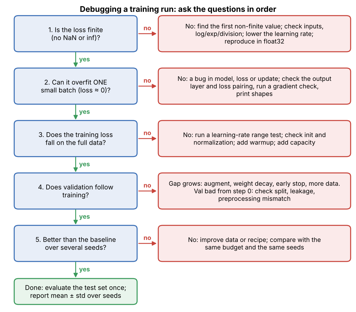
Overfit one batch first
Plain version. Take one small batch and train on it over and over. A correct model and training loop can memorize a handful of images, so the loss must fall to nearly zero. If it cannot, something is broken, and you have found that out in seconds instead of days.
Karpathy’s recipe for training networks puts this test early: overfit a single small batch, and before that, check that the loss at initialization is what it should be [2]. For balanced classes and a well-initialized final layer, the first predictions are close to uniform, so the cross-entropy starts near ( for our digits). The snippet checks that, then runs the one-batch test on 16 digits twice: once correctly, and once with a bug that is easy to make, applying softmax in the model and inside the loss. It reuses init and forward from the running example.
Code · Python · 29 lines
def overfit_one_batch(double_softmax=False, steps=300, lr=0.1, seed=0):
    P = init(seed)
    xb, yb = X_tr[:16], y_tr[:16]                       # ONE fixed batch of 16 images
    for step in range(steps):
        h = forward(P, xb)
        z = h[-1]
        if double_softmax:                              # BUG: the "logits" are already probabilities
            z = np.exp(z - z.max(1, keepdims=True))
            z = z / z.sum(1, keepdims=True)
        s = z - z.max(1, keepdims=True)
        p = np.exp(s) / np.exp(s).sum(1, keepdims=True)
        loss = -np.log(p[np.arange(16), yb]).mean()
        d = p.copy()
        d[np.arange(16), yb] -= 1
        d /= 16
        if double_softmax:                              # chain rule through the extra softmax
            d = z * (d - (d * z).sum(1, keepdims=True))
        for i in reversed(range(len(P))):
            gW, gb = h[i].T @ d, d.sum(0)
            if i:
                d = (d @ P[i][0].T) * (h[i] > 0)
            P[i][0] -= lr * gW
            P[i][1] -= lr * gb
    return loss

print(f"loss at init:          {evaluate(init(0), X_tr, y_tr)[0]:.4f}   (ln 10 = {np.log(10):.4f})")
print(f"correct loss:          {overfit_one_batch():.4f}")
print(f"double-softmax bug:    {overfit_one_batch(double_softmax=True):.4f}")
print(f"floor of the bug:      {-np.log(np.e / (np.e + 9)):.4f}")
Output
loss at init:          2.8204   (ln 10 = 2.3026)
correct loss:          0.0036
double-softmax bug:    1.4661
floor of the bug:      1.4612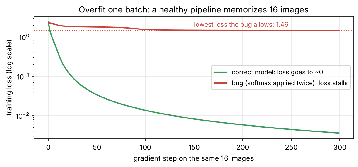
The initial loss is somewhat above because the He-initialized output layer produces logits of moderate size, so the first predictions are not exactly uniform; that is harmless here. A value far above means the network starts out confidently wrong, and scaling the last layer’s initial weights down fixes it. The bug has a hard floor. After the first softmax, the “logits” passed to the loss lie between 0 and 1, so the best the second softmax can do is give the true class against for each of the nine others: a probability of and a loss of . On the full dataset this bug does not crash and still produces a usable classifier, so it can go unnoticed; the one-batch test exposes it in seconds.
A passing test proves less than it seems. Zhang et al. showed that standard image classifiers can fit random labels, and even random noise images, perfectly [36], so memorizing one batch says that the model, the loss and the update can learn, not that the labels are correct. Mislabeled or misaligned data must be caught by looking at it (checklist item 2).
Reading loss curves
Plain version. A loss curve is the main record of a run: its shape tells you which part of the pipeline to suspect. Plot training and validation curves together, on a log scale for the loss.
ML 02 explains the four basic shapes (flat, overfitting, converged, healthy). A few more patterns are typical of vision training:
- Stuck exactly at . The network outputs uniform probabilities: the gradient is not reaching it (a detached tensor, frozen parameters, a learning rate of zero) or the labels are constant.
- Loss spikes that recover. The learning rate is near the edge of stability, as in Figure 4, or a few batches contain corrupted images or labels. Log the indices of the batches with the largest loss and look at them.
- Validation better than training. Normal with strong augmentation or dropout, because the training loss is measured on harder, augmented inputs.
- Validation accuracy flat while validation loss rises. The network becomes overconfident on the examples it gets wrong; the ranking is fine, but the probabilities are not (calibration in DLCV 02).
- A drop at every milestone. Expected with step decay. If the curve is still falling steeply at the end of a cosine schedule, the budget is too short.
- Good validation, bad deployment. Suspect a preprocessing mismatch, or shortcut learning: the network relies on a cue that the validation set shares with the training set but deployment data lacks [37] (DLCV 02).
Gradient norms, dead units and NaNs
Plain version. Log a few health numbers every few hundred steps: the size of each layer’s gradient, the fraction of units that never activate, and whether anything has become NaN. When training goes wrong, these numbers usually go wrong first.
The snippet computes two of them after three epochs at three constant learning rates. It reuses train, forward, loss_and_grads and constant from above.
Code · Python · 12 lines
def health(P, X, y):
    _, G = loss_and_grads(P, X, y)
    h = forward(P, X)[1]                                # hidden ReLU activations
    dead = (h.max(0) == 0).mean()                       # units that are zero for every input
    norms = [np.linalg.norm(gW) for gW, _ in G]
    return norms, dead

for peak in (0.01, 0.1, 0.3):
    P, log, _ = train(constant, peak=peak, epochs=3)
    norms, dead = health(P, X_tr, y_tr)
    print(f"lr {peak:<5} train loss {log[-1, 0]:9.3g}  grad norms "
          f"{norms[0]:9.3g} {norms[1]:9.3g}  dead units {dead:.0%}")
Output
lr 0.01  train loss     0.127  grad norms    0.0664    0.0496  dead units 0%
lr 0.1   train loss      3.61  grad norms      1.44      2.11  dead units 0%
lr 0.3   train loss   2.1e+08  grad norms  1.02e+04  1.31e+04  dead units 0%
The gradient norms grow by more than five orders of magnitude between the healthy and the diverging run, long before the loss becomes NaN, so logging them is cheap insurance. Gradient clipping (ML 02) is a sensible guard, but it hides a too-large learning rate rather than fixing it. No units die here, because this toy fails by explosion. A dead ReLU outputs zero for every input, so it gets no gradient and never recovers; many dead units, typically after a huge step or with strongly negative biases, mean lost capacity.
When the loss becomes NaN or infinite, find the first operation that produced a non-finite value rather than clipping everything: check inputs, then the forward pass, the loss, the gradients and the update size, and reproduce in float32 before blaming mixed precision. ML 01C gives this order in detail, and its section on checking derivatives shows how to test a hand-written backward pass.
Reproducibility and fair experiments
Plain version. A result is only useful if it can be repeated and if the comparison behind it is fair. Fix the seeds, log what you did, and run each setting several times, because random chance alone can move a score by more than the improvement you hope to show.
Seeds, determinism and logging
Seed every random number generator: Python’s, NumPy’s, the framework’s and the data-loader workers’. Even then, runs can differ: the PyTorch documentation states that completely reproducible results are not guaranteed across releases, commits or platforms, or between CPU and GPU. Within one setup it recommends torch.use_deterministic_algorithms(True), disabling cuDNN benchmarking, and seeding data-loader workers through worker_init_fn and a generator, and it warns that deterministic operations are often slower [38]. Log enough to rerun the experiment: code version, configuration, data version and split identifiers, seeds, environment and hardware, and the curves of loss, metrics, learning rate and gradient norm (ML 11).
How much do seeds matter?
The seed changes the initialization and the order of the data, and therefore the result. The snippet trains two configurations on the toy, A (warmup + cosine) and B (one-cycle), each with five seeds, and compares them pair by pair (it reuses train and the schedule functions):
Code · Python · 8 lines
seeds = range(5)
A = [train(warmup_cosine, peak=0.1, seed=s)[1][-1, 3] for s in seeds]
B = [train(one_cycle, peak=0.1, seed=s)[1][-1, 3] for s in seeds]
print("A (warmup + cosine):", np.round(A, 3))
print("B (one-cycle):      ", np.round(B, 3))
d = np.array(B) - np.array(A)                           # paired: same seed, same data order
print(f"A mean {np.mean(A):.3f} +- {np.std(A, ddof=1):.3f}   B mean {np.mean(B):.3f} +- {np.std(B, ddof=1):.3f}")
print(f"paired difference B - A: mean {d.mean():+.3f}, range {d.min():+.3f} to {d.max():+.3f}")
Output
A (warmup + cosine): [0.971 0.962 0.956 0.956 0.959]
B (one-cycle):       [0.956 0.952 0.952 0.978 0.956]
A mean 0.961 +- 0.007   B mean 0.959 +- 0.011
paired difference B - A: mean -0.002, range -0.016 to +0.022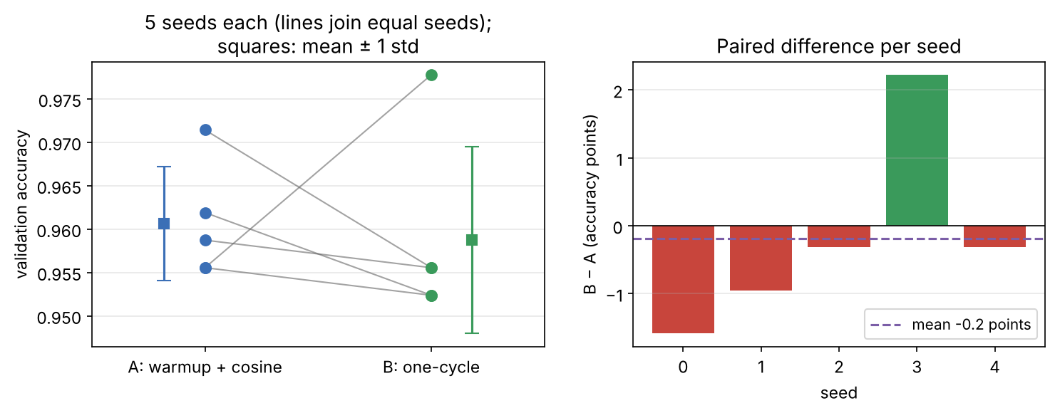
With only seed 3 you would report that one-cycle wins by 2.2 points; with seed 0, that it loses by 1.6. Over five seeds the mean difference is 0.2 points with a spread far larger than that: no detectable difference on this toy (and one validation image is worth about 0.3 points here). Report the mean and standard deviation over seeds, compare configurations paired on the same seeds and splits, and use the confidence intervals and paired tests of ML 11 before claiming an improvement. Published large-scale results do this too: Goyal et al. report every ImageNet error as a mean and standard deviation over five trials [9].
Baselines, ablations and budgets
A fair experiment changes one thing and holds everything else fixed:
- Baselines. Always include a simple baseline and the previous best recipe, trained by you in the same pipeline. A new method compared with a baseline from an old paper mixes the effect of the method with the effect of the recipe (DLCV 02).
- Equal tuning budget. Give every method the same number of trials for its hyperparameters. A method tuned for a week against a baseline run once wins by tuning, not by design.
- Equal training budget. Compare at the same number of steps or the same compute; a longer schedule alone can explain a gain.
- Ablations. Remove one component at a time from the full method, with several seeds each, and report the drop. An ablation that changes two things at once cannot tell you which one mattered.
- One test evaluation. Make every decision on validation data; evaluate the final choice on the test set once.
The Deep Learning Tuning Playbook organizes this into an incremental strategy: decide on the goal of each round of experiments, separate the hyperparameters being studied from those that must be re-tuned for each setting (“nuisance” hyperparameters) and those held fixed, and adopt a change only when the evidence is strong [26].
Modern view
Plain version. The core habits of this chapter are stable. Recent work changes how training methods are compared, how much of the schedule must be fixed in advance, and how large pretrained models are adapted.
What the surveys and guides say
Practical training knowledge lives more in reviews and guides than in single papers. Bengio’s chapter in Neural Networks: Tricks of the Trade collects recommendations for gradient-based training, from the learning rate and mini-batch size to early stopping and hyperparameter search [12]. The Deep Learning Tuning Playbook covers choosing the architecture, optimizer, batch size and initial configuration, an incremental, scientific tuning process, how long to train, and pipeline details such as checkpoint selection and experiment tracking [26]. Shorten and Khoshgoftaar organize image augmentation into geometric and color transformations, kernel filters, mixing images, random erasing, feature-space and adversarial augmentation, generative and style-transfer augmentation, and meta-learned policies, and also discuss test-time augmentation [7]. Xin et al. divide parameter-efficient fine-tuning of vision models into addition-based, partial-based, unified-based and multi-task tuning, and propose a unified benchmark [39].
Comparing training methods fairly is itself hard. Dahl et al. argue that the community cannot reliably identify training-algorithm improvements, because it is unclear when training is complete, results are sensitive to workload details, and methods that need tuning are hard to compare fairly; they introduced the AlgoPerf benchmark, which measures time to reach a target result on fixed hardware across several workloads [40].
The state of the art, 2023–2026
- Benchmarked training algorithms. The first AlgoPerf competition drew 18 submissions from 10 teams. In the ruleset where submitters provide a search space, the winner used non-diagonal preconditioning and beat popular methods such as Adam even on wall-clock time; in the ruleset with no tuning allowed, the winner was based on Schedule-Free AdamW [41].
- Fewer schedules to tune. Defazio et al.’s Schedule-Free approach removes the need to know the stopping step in advance by unifying scheduling and iterate averaging, without new hyperparameters beyond those of momentum optimizers [42]. A simpler alternative is a constant learning rate followed by a short “cooldown” decay, named warmup-stable-decay (WSD) in MiniCPM [43]. Hägele et al. found that this scales as predictably as a cosine schedule, that a cooldown over a modest fraction of training is enough, and that weight averaging improves results along the trajectory at no extra training cost; their experiments are on language models, so verify the transfer to vision workloads yourself [44].
- Weight averaging everywhere. Beyond the EMA study above [29], averaging is also used in fine-tuning: WiSE-FT interpolates between the zero-shot and fine-tuned weights of a pretrained model and improves robustness under distribution shift [45], and model soups average several fine-tuned models to improve accuracy without extra inference cost [46].
- Fine-tuning foundation models. With very large pretrained backbones, full fine-tuning can be replaced by linear probing, LP-FT [35], or parameter-efficient methods such as LoRA [33], [39]. The practical questions shift from “which architecture” to “which pretrained model, and how much of it to adapt”.
Open problems
- Hyperparameters that transfer. Best learning rates, warmup lengths and weight decays still change with model size, batch size and dataset; the range test and the linear scaling rule are approximations, not laws.
- Fair, affordable comparison. Tuning budgets differ between papers, and seeds are often too few to separate methods. Benchmarks such as AlgoPerf address this for training algorithms [40], but no comparable standard exists for most vision tasks.
- Determinism at scale. Bit-exact reproducibility is not guaranteed across hardware and software versions [38], which makes small regressions hard to diagnose in large training runs.
- Augmentation for dense and specialized tasks. How to choose augmentation automatically for detection, segmentation, medical and remote-sensing images, where geometry and intensity carry label information, is still an open question.
- Fine-tuning without forgetting. Adapting a foundation model to a narrow task while keeping its robustness out of distribution is still an active research question [35], [45].
Key takeaways
- Inspect a processed batch, check the initial loss and overfit one batch before scaling up.
- Split by the deployment unit, fit preprocessing on training data, and transform spatial labels with the image.
- Use a learning-rate range test, warmup and decay; recheck the schedule when batch size changes.
- Accumulation matches a larger batch only under compatible loss weighting and batch-dependent operations; normalize by the actual sample, pixel or box count.
- Tune interacting regularizers together and select checkpoints using validation data.
- Fine-tune pretrained features gently and check normalization behavior with small batches.
- Report multiple seeds, matched budgets and isolated ablations; reserve the test set for final evaluation.
Exercises
- Range test, then schedule. Rerun the range test with batch sizes 8, 16 and 64 (change
bs). How does the learning rate of the minimum move? Then train withwarmup_cosineat each batch size, using a peak taken from its own range test, and compare with the linear scaling rule.
Hint
In our runs (seeds 0 and 1) the minimum sat at about 0.15–0.16 for batch 8, 0.13–0.14 for batch 16 and 0.35 for batch 64: it moves up with the batch size, but not in exact proportion, and a short test is noisy. Remember that in steps shrinks as the batch grows at a fixed number of epochs, so the larger batches also get fewer updates.
- A one-batch test that passes for the wrong reason. Shuffle
y_tr[:16](so labels no longer match images) and runoverfit_one_batch. What happens to the loss, and what does that tell you about what the test can and cannot detect? Which check from the checklist would have caught the shuffled labels?
Hint
The loss still goes to nearly zero (0.0056 in our run with the labels permuted by np.random.default_rng(0)), because a network can memorize any 16 labels, as Zhang et al. showed for random labels at scale [36]. The test checks the model, the loss and the update, not the data. Looking at a batch with its labels drawn on it (item 2) catches misaligned labels; so does a validation accuracy near chance.
- Flip a keypoint. Extend the
hflipfunction so it also transforms a list of keypoints given as(x, y, name)with names such asleft_eyeandright_eye. Write a check that fails if a flippedleft_eyeis still calledleft_eye.
Hint
The coordinates follow for pixel centers (or for continuous coordinates, matching the box convention used here), unchanged. Then swap every left/right name pair with a lookup table. Applying the flip twice must return the original keypoints exactly, which is a good test.
- Accumulation with ignored pixels. A segmentation loss averages the per-pixel cross-entropy over pixels whose label is not “ignore”. Micro-batch 1 has 1,000 valid pixels with mean loss 0.5; micro-batch 2 has 3,000 valid pixels with mean loss 0.9. What is the mean loss of the combined batch, and what does averaging the two micro-batch means give instead?
Hint
The combined mean is . Averaging the means gives , which underweights the micro-batch with more valid pixels. The same weighting applies to the gradients: accumulate sums and divide by the total count.
- How many seeds? Using
train, run configurations A and B with 10 seeds each instead of 5. Does the mean difference change sign? Estimate the standard error of the paired mean difference, , where is the standard deviation of the per-seed differences and the number of seeds, and decide whether a 0.5-point improvement could be detected with 10 seeds.
Hint
In our run with seeds 0–9 the sign does change: the mean difference B − A becomes about +0.6 points, against −0.2 points with five seeds. With points, the standard error is points, so a 0.5-point improvement is only about one standard error away from zero: not convincing. Larger validation sets and more seeds both help; ML 10 shows paired bootstrap intervals.
- Fine-tuning plan. You have 2,000 labeled X-ray images, a backbone pretrained on natural photos and one GPU that fits 8 images per batch. Write a training plan: normalization statistics, augmentations (which ones are unsafe?), how to handle batch normalization, the fine-tuning strategy, the learning-rate procedure and how you will decide that a change helped.
Hint
Use the pretrained normalization statistics; avoid intensity augmentations that change diagnostic values, and be careful with flips if laterality matters; freeze the backbone BN statistics (or use group normalization in new layers) because 8 images per batch give noisy statistics; start with a linear probe, then LP-FT with smaller rates for early layers and a short warmup; run a range test for the head; split by patient; compare variants over several seeds with paired intervals.
References
- T. He, Z. Zhang, H. Zhang, Z. Zhang, J. Xie and M. Li, “Bag of tricks for image classification with convolutional neural networks,” in Proc. IEEE/CVF CVPR, 2019. doi
- A. Karpathy, “A recipe for training neural networks,” blog post, 2019. link
- scikit-learn developers, “load_digits,” scikit-learn documentation, version 1.9.1. link
- M. Buda, A. Maki and M. A. Mazurowski, “A systematic study of the class imbalance problem in convolutional neural networks,” Neural Networks, vol. 106, 2018. doi
- T.-Y. Lin, P. Goyal, R. Girshick, K. He and P. Dollár, “Focal loss for dense object detection,” in Proc. IEEE ICCV, 2017. doi
- A. Buslaev, V. I. Iglovikov, E. Khvedchenya, A. Parinov, M. Druzhinin and A. A. Kalinin, “Albumentations: Fast and flexible image augmentations,” Information, vol. 11, no. 2, 2020. doi
- C. Shorten and T. M. Khoshgoftaar, “A survey on image data augmentation for deep learning,” Journal of Big Data, vol. 6, 2019. doi
- K. He, X. Zhang, S. Ren and J. Sun, “Delving deep into rectifiers: Surpassing human-level performance on ImageNet classification,” in Proc. IEEE ICCV, 2015. doi
- P. Goyal, P. Dollár, R. Girshick, P. Noordhuis, L. Wesolowski, A. Kyrola, A. Tulloch, Y. Jia and K. He, “Accurate, large minibatch SGD: Training ImageNet in 1 hour,” arXiv:1706.02677 (technical report), 2017. arXiv
- S. Ioffe and C. Szegedy, “Batch normalization: Accelerating deep network training by reducing internal covariate shift,” in Proc. ICML, PMLR 37, 2015. link
- Y. Wu and K. He, “Group normalization,” in Proc. ECCV, 2018. doi
- Y. Bengio, “Practical recommendations for gradient-based training of deep architectures,” in Neural Networks: Tricks of the Trade, 2nd ed., LNCS 7700, Springer, 2012. doi
- L. N. Smith, “Cyclical learning rates for training neural networks,” in Proc. IEEE WACV, 2017. doi
- L. N. Smith, “A disciplined approach to neural network hyper-parameters: Part 1 — learning rate, batch size, momentum, and weight decay,” US Naval Research Laboratory Technical Report 5510-026, arXiv:1803.09820, 2018. arXiv
- I. Loshchilov and F. Hutter, “SGDR: Stochastic gradient descent with warm restarts,” in Proc. ICLR, 2017. arXiv
- L. N. Smith and N. Topin, “Super-convergence: Very fast training of neural networks using large learning rates,” in Artificial Intelligence and Machine Learning for Multi-Domain Operations Applications, Proc. SPIE 11006, 2019. doi
- PyTorch contributors, “torch.optim.lr_scheduler.OneCycleLR,” PyTorch 2.15 documentation, 2026. link
- K. He, X. Zhang, S. Ren and J. Sun, “Deep residual learning for image recognition,” in Proc. IEEE CVPR, 2016. doi
- J. Deng, W. Dong, R. Socher, L.-J. Li, K. Li and L. Fei-Fei, “ImageNet: A large-scale hierarchical image database,” in Proc. IEEE CVPR, 2009. doi
- D. P. Kingma and J. Ba, “Adam: A method for stochastic optimization,” in Proc. ICLR, 2015. arXiv
- I. Loshchilov and F. Hutter, “Decoupled weight decay regularization,” in Proc. ICLR, 2019. arXiv
- PyTorch contributors, “torch.optim.Adam,” PyTorch 2.15 documentation, 2026. link
- N. Srivastava, G. Hinton, A. Krizhevsky, I. Sutskever and R. Salakhutdinov, “Dropout: A simple way to prevent neural networks from overfitting,” Journal of Machine Learning Research, vol. 15, 2014. link
- G. Huang, Y. Sun, Z. Liu, D. Sedra and K. Q. Weinberger, “Deep networks with stochastic depth,” in Proc. ECCV, 2016. doi
- L. Prechelt, “Early stopping — but when?,” in Neural Networks: Tricks of the Trade, 2nd ed., LNCS 7700, Springer, 2012. doi
- V. Godbole, G. E. Dahl, J. Gilmer, C. J. Shallue and Z. Nado, “Deep learning tuning playbook,” Google Research, GitHub repository, 2023. link
- B. T. Polyak and A. B. Juditsky, “Acceleration of stochastic approximation by averaging,” SIAM Journal on Control and Optimization, vol. 30, no. 4, 1992. doi
- P. Izmailov, D. Podoprikhin, T. Garipov, D. Vetrov and A. G. Wilson, “Averaging weights leads to wider optima and better generalization,” in Proc. UAI, 2018. arXiv
- D. Morales-Brotons, T. Vogels and H. Hendrikx, “Exponential moving average of weights in deep learning: Dynamics and benefits,” Transactions on Machine Learning Research, 2024. arXiv
- P. Micikevicius, S. Narang, J. Alben, G. Diamos, E. Elsen, D. Garcia, B. Ginsburg, M. Houston, O. Kuchaiev, G. Venkatesh and H. Wu, “Mixed precision training,” in Proc. ICLR, 2018. arXiv
- PyTorch contributors, “Automatic mixed precision package — torch.amp,” PyTorch 2.15 documentation, 2026. link
- J. Yosinski, J. Clune, Y. Bengio and H. Lipson, “How transferable are features in deep neural networks?,” in Advances in Neural Information Processing Systems 27, 2014. link
- E. J. Hu, Y. Shen, P. Wallis, Z. Allen-Zhu, Y. Li, S. Wang, L. Wang and W. Chen, “LoRA: Low-rank adaptation of large language models,” in Proc. ICLR, 2022. arXiv
- J. Howard and S. Ruder, “Universal language model fine-tuning for text classification,” in Proc. ACL, 2018. doi
- A. Kumar, A. Raghunathan, R. Jones, T. Ma and P. Liang, “Fine-tuning can distort pretrained features and underperform out-of-distribution,” in Proc. ICLR, 2022. arXiv
- C. Zhang, S. Bengio, M. Hardt, B. Recht and O. Vinyals, “Understanding deep learning requires rethinking generalization,” in Proc. ICLR, 2017. arXiv
- R. Geirhos, J.-H. Jacobsen, C. Michaelis, R. Zemel, W. Brendel, M. Bethge and F. A. Wichmann, “Shortcut learning in deep neural networks,” Nature Machine Intelligence, vol. 2, 2020. doi
- PyTorch contributors, “Reproducibility,” PyTorch 2.15 documentation, 2026. link
- Y. Xin, J. Yang, S. Luo, Y. Du, Q. Qin, K. Cen, Y. He, Z. Zhang, B. Fu, X. Yang, G. Zhai, M.-H. Yang and X. Liu, “Parameter-efficient fine-tuning for pre-trained vision models: A survey and benchmark,” arXiv:2402.02242, 2024. arXiv
- G. E. Dahl, F. Schneider, Z. Nado, N. Agarwal, C. S. Sastry, P. Hennig, S. Medapati, R. Eschenhagen, P. Kasimbeg, D. Suo et al., “Benchmarking neural network training algorithms,” arXiv:2306.07179, 2023. arXiv
- P. Kasimbeg, F. Schneider, R. Eschenhagen, J. Bae, C. S. Sastry, M. Saroufim, B. Feng, L. Wright, E. Z. Yang, Z. Nado, S. Medapati, P. Hennig, M. Rabbat and G. E. Dahl, “Accelerating neural network training: An analysis of the AlgoPerf competition,” in Proc. ICLR, 2025. arXiv
- A. Defazio, X. A. Yang, H. Mehta, K. Mishchenko, A. Khaled and A. Cutkosky, “The road less scheduled,” in Advances in Neural Information Processing Systems 37, 2024. link
- S. Hu, Y. Tu, X. Han, C. He, G. Cui, X. Long, Z. Zheng, Y. Fang, Y. Huang, W. Zhao et al., “MiniCPM: Unveiling the potential of small language models with scalable training strategies,” in Proc. Conference on Language Modeling (COLM), 2024. arXiv
- A. Hägele, E. Bakouch, A. Kosson, L. Ben Allal, L. Von Werra and M. Jaggi, “Scaling laws and compute-optimal training beyond fixed training durations,” in Advances in Neural Information Processing Systems 37, 2024. link
- M. Wortsman, G. Ilharco, J. W. Kim, M. Li, S. Kornblith, R. Roelofs, R. Gontijo Lopes, H. Hajishirzi, A. Farhadi, H. Namkoong and L. Schmidt, “Robust fine-tuning of zero-shot models,” in Proc. IEEE/CVF CVPR, 2022. doi
- M. Wortsman, G. Ilharco, S. Y. Gadre, R. Roelofs, R. Gontijo-Lopes, A. S. Morcos, H. Namkoong, A. Farhadi, Y. Carmon, S. Kornblith and L. Schmidt, “Model soups: Averaging weights of multiple fine-tuned models improves accuracy without increasing inference time,” in Proc. ICML, PMLR 162, 2022. link
- PyTorch contributors, “Automatic mixed precision examples,” PyTorch 2.15 documentation, 2026. link
- PyTorch contributors, “DistributedDataParallel,” PyTorch 2.15.0 source documentation, 2026. Official source.
Check your understanding
This tutorial has 6 exercises. Can you solve them without opening the hints?
Go to the exercises ↑Next DLCV 01B · Building Blocks and How to Compose Them: Classification and Restoration Networks · 42 min