DLCV 09B · Generative Image Restoration: Sampling a Plausible Answer
Needs: DLCV 09 · Deep Image Restoration: Low-Level Vision, ML 07 · Generative Models: Autoencoders, VAEs, GANs and Flows
Navigate: this page and this track: Navigate: this page and this track
On this page
- What you’ll learn1 min
- The big picture2 min
- Why regression gives blur: the posterior mean3 min
- What “generative” restoration means2 min
- The perception–distortion trade-off3 min
- Family 1: GAN-based restoration and GAN priors3 min
- Family 2: diffusion models as priors9 min
- Family 3: latent-diffusion and foundation-model restorers3 min
- Family 4: flow matching and rectified flow restorers1 min
- Evaluating generative restoration3 min
- Failure modes and when NOT to use generative restoration2 min
- Modern view3 min
- Key takeaways1 min
- Exercises4 min
- Supplementary notes
- Paper guides
- References
- Blau and Michaeli, “The Perception-Distortion Tradeoff” (CVPR 2018)
- Chung et al., “Diffusion Posterior Sampling for General Noisy Inverse Problems” (ICLR 2023)
- DDNM: preserve measured components and generate the null space
- BlindDPS: infer an image and its degradation together
- Li et al., “Diffusion Models for Image Restoration and Enhancement: A Comprehensive Survey” (IJCV 2025)
Deep Learning for Computer Vision
Explore this chapter 1 interactive experiment
A blurry observation fits two sharp clean signals. The blurry average has the lowest expected squared error; a sharp guess looks better but is usually farther from the truth.
What you’ll learn
- Explain why squared-error restoration averages uncertain detail.
- Distinguish plausible posterior samples from faithful recovery.
- Compare GAN priors, conditional diffusion and pretrained-prior inverse solvers.
- Trace prior guidance and measurement consistency in a runnable toy example.
- Evaluate randomness, hallucination and complete inference cost.
The big picture
DLCV 09 trained restoration networks to be close to the clean image on average. That works well for mild damage. When the damage destroys a lot of information (a 16-pixel-wide face, a heavily compressed photo, a large hole), “close on average” produces a smooth, waxy guess. Generative restoration takes a different stance: since many clean images are consistent with the input, pick one of them, and make sure it looks like a real photo.
Why it matters. The most convincing real-world super-resolution and face or old-photo restoration of recent years comes from generative models, GANs first and diffusion models since about 2021. The same machinery is used for medical and scientific inverse problems, where an invented detail can do real harm. So you need two skills at once: how these methods work, and how to measure what they invent.
Where this chapter sits. It builds on the degradation model, losses and metrics of DLCV 09 and the generative models of ML 07; diffusion and flow matching are derived in ML 08, and here we only use them. Super-resolution, which has its own chapters (DLCV 09A for images, DLCV 09A.3 for video), appears here only as an example. All code runs in seconds on a CPU with NumPy and SciPy, on toy problems whose exact answer is known, so every claim can be checked.
Why regression gives blur: the posterior mean
Plain version. Squared-error training favors the conditional average. When several sharp structures explain the same input, their average can be blurry.
One input, many answers
Write the measurement as , as in DLCV 09. For super-resolution, deblurring, inpainting or heavy compression, throws information away, so a whole set of clean images explains the same almost equally well. In the Bayesian language, the uncertainty that remains after seeing is the posterior distribution
where is the prior (how likely an image is before we look at : natural images are likely, noise is not), is the likelihood (how well explains the measurement; for Gaussian noise of standard deviation it is proportional to ), and is a normalizing constant that does not depend on . Mild damage gives a narrow posterior, and every reasonable method agrees. Severe damage gives a wide posterior, often with several separate modes (“the edge is here” or “two pixels to the right”).
The math: squared error is minimized by the posterior mean
A restoration network trained on pairs with the squared error minimizes the expected loss over the data distribution. For each fixed , the best output minimizes
where the expectation is over the posterior and is the posterior mean. The second term does not depend on (it is the irreducible uncertainty), so the minimum is at
the minimum mean squared error (MMSE) estimator. A large enough network trained long enough approaches it. (The L1 loss gives the per-pixel posterior median instead: sometimes sharper, but still chosen pixel by pixel rather than as one coherent image; DLCV 09 compares the losses.) The posterior mean is the right answer if you are scored by MSE or PSNR, and the wrong one if you want an image that looks real: averaging images with edges in different places gives an image with no sharp edge at all.
Code: a toy where the mean is blurry and every sample is sharp
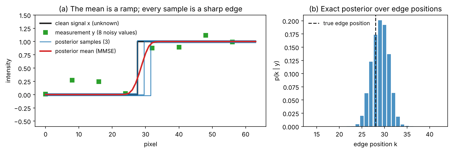
We need a problem whose posterior we can compute exactly. The clean “images” are 1-D signals of 64 pixels with one step edge (0 on the left, 1 on the right) at an unknown position between pixels 8 and 55, all equally likely. The degradation blurs with a Gaussian of standard deviation 3 pixels, keeps one pixel in eight and adds Gaussian noise of standard deviation 0.2. With only 48 possible clean signals, the posterior is an exact list of 48 probabilities.
Code · Python · 37 lines
import numpy as np
from scipy.ndimage import gaussian_filter1d
from scipy.stats import wasserstein_distance

rng = np.random.default_rng(0)
n, factor, sigma = 64, 8, 0.2
positions = np.arange(8, 56)                                     # where the edge may be
X = (np.arange(n)[None, :] >= positions[:, None]).astype(float)  # every possible clean signal
A = lambda x: gaussian_filter1d(x, 3.0, axis=-1, mode="nearest")[..., ::factor]  # blur, keep 1 of 8
AX = A(X)                                                        # every candidate, degraded

def posterior(y):
    """Exact p(edge position | y): uniform prior, Gaussian noise of std sigma."""
    logp = -np.sum((y - AX) ** 2, axis=1) / (2 * sigma**2)
    p = np.exp(logp - logp.max())
    return p / p.sum()

truth, mean, post, prior = [], [], [], []
for _ in range(2000):
    x = X[rng.integers(len(positions))]
    y = A(x) + sigma * rng.standard_normal(n // factor)
    p = posterior(y)
    truth.append(x)
    mean.append(p @ X)                                           # posterior mean (MMSE)
    post.append(X[rng.choice(len(positions), p=p)])              # a sample from p(x | y)
    prior.append(X[rng.integers(len(positions))])                # a sample that ignores y
truth = np.array(truth)

for name, est in [("posterior mean", mean), ("posterior sample", post), ("prior sample", prior)]:
    est = np.array(est)
    mse = np.mean((est - truth) ** 2)
    w1 = wasserstein_distance(est.ravel(), truth.ravel())        # pixel values like real ones?
    jump = np.abs(np.diff(est, axis=1)).max(axis=1).mean()       # sharpest step (real: 1.0)
    print(f"{name:16s} MSE {mse:.4f} | W1 {w1:.4f} | largest step {jump:.2f}")
# posterior mean   MSE 0.0169 | W1 0.0243 | largest step 0.22
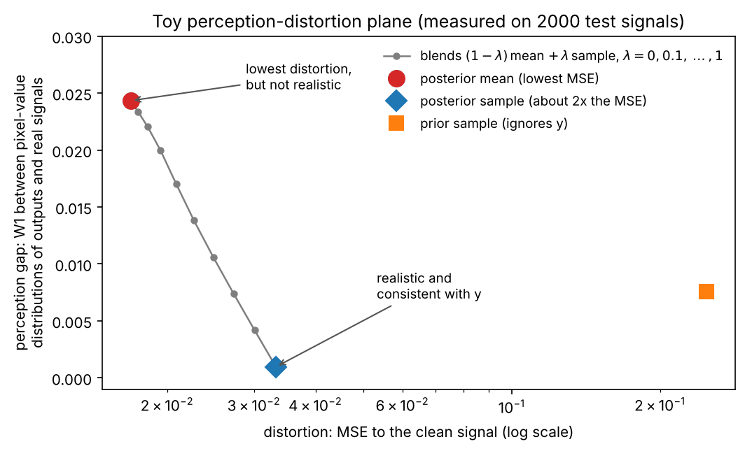
# posterior sample MSE 0.0333 | W1 0.0010 | largest step 1.00
# prior sample     MSE 0.2485 | W1 0.0076 | largest step 1.00
Three estimators are compared over 2,000 random test signals. The columns are the MSE to the clean signal; a crude “realism” score, the 1-D Wasserstein distance W1 between the distribution of output pixel values and that of real pixel values (real signals contain only 0s and 1s, so in-between gray values are unrealistic); and the height of the sharpest step in the output (1.0 for every real signal). All numbers in this chapter’s code blocks come from our own runs.
- The posterior mean has the lowest MSE, but its sharpest step averages 0.22: it is a ramp, not an edge, and its gray values make it statistically unlike any real signal.
- A posterior sample is a real edge (step 1.00, W1 near zero) placed where the data allow. Its MSE is 0.0333, almost exactly twice the posterior mean’s 0.0169. That factor of two is not a coincidence (next section).
- A prior sample ignores . It is perfectly realistic and useless: its MSE is about 15 times worse. Realism alone is not restoration. (Its W1 of 0.0076 instead of 0 is sampling noise of the 2,000-signal test.)
What “generative” restoration means
Plain version. A generative restorer selects a plausible answer. An ideal posterior sampler would reproduce the input’s conditional uncertainty across repeated draws.
Precise version. A generative (or stochastic, or posterior-sampling) restorer is a random map: given and a random seed , it returns whose distribution, for fixed , is meant to approximate . Three ingredients appear in every method of this chapter:
- A prior of natural images, learned by a generative model (a GAN, a diffusion model, a flow, a codebook).
- A likelihood or data-consistency term that ties the output to the input, either explicitly ( with a known ) or implicitly (a network that is shown and trained on pairs).
- A way to produce samples: one forward pass of a generator, or many steps of a sampler.
A convenient identity connects the three. Taking the gradient of the logarithm of Bayes’ rule with respect to removes the constant :
where is the score of the prior (a vector field pointing toward more likely images) and is the gradient of the likelihood (pointing toward images that explain better). Every sampler that follows “uphill directions plus noise” can therefore be split into a prior push and a data push. This split is the backbone of zero-shot diffusion restoration below.
There are two broad ways to build such a restorer:
- Learn the posterior directly (supervised): train a conditional generator on pairs , as conditional GANs and conditional diffusion models do. never has to be written down, but a new degradation needs new training.
- Combine a prior with a known likelihood (zero-shot): train an unconditional generative model on clean images once, then steer its sampler with and at test time, as GAN inversion and DPS-type methods do. One model serves many tasks, but must be known and sampling is usually slower.
The perception–distortion trade-off
Plain version. Realistic samples commit to uncertain detail. Under the ideal exact-posterior assumptions, sampling has twice the optimal mean estimator’s expected MSE; learned generators have no such guarantee.
Precise version. Blau and Michaeli [1] define, for any restoration method that outputs from , its distortion , where is any per-image distortion measure such as squared error, and its perceptual quality as a divergence between the distribution of real images and the distribution of restored images (zero means the outputs are statistically indistinguishable from real images, for example by a perfect discriminator). The perception–distortion function is
where the minimum is over all, possibly random, restoration methods and is the distortion budget. They prove that is non-increasing, and convex when is convex in its second argument [1]. So there is an unattainable region near the origin of the (distortion, perception) plane: lowering distortion past a point forces outputs away from the real-image distribution. They also show that this holds for any distortion measure, not only for MSE.
Two points on the curve matter most. Let be the lowest possible distortion (achieved by the MMSE estimator for squared error) and the lowest distortion achievable with perfect perceptual quality (). For squared error the paper proves (in its extended arXiv version [1])
and the bound is reached by posterior sampling, . In PSNR terms, perfect realism never needs to cost more than about 3 dB, because . This is exactly the factor of two in our toy (0.0333 versus 0.0169). The paper also notes that the bound need not be tight: some problems allow perfect realism for less than twice the MMSE.
Optional: Why posterior sampling exactly doubles the MSE (in the Supplementary notes). A four-line proof of the factor of two.
Figure 2 places the toy’s estimators on the plane. Between the posterior mean and the posterior sample we also plot simple blends , a simple way to trade the two. Their expected MSE is , because a posterior sample’s deviation from the mean is uncorrelated with the truth’s deviation, so gives the factor of two. The blends are one achievable path; the true bound may lie below it.
What this means in practice:
- A method is a point, not a score. Report a distortion metric (PSNR, SSIM) and a perceptual one, and say which point your method aims for. Comparing a GAN restorer with an MSE restorer by PSNR alone is comparing two different targets.
- “Better PSNR and better realism” is possible only for methods away from the bound. Once a method is near the curve, it can only move along it.
- Many generative restorers expose a knob that slides along the curve: a GAN loss weight, a fidelity weight in CodeFormer [10], a feature-wrapping scalar in StableSR [24], a guidance scale in DiffBIR [25]. Choosing the knob is choosing a point on the trade-off.
Optional: Blau and Michaeli, “The Perception-Distortion Tradeoff” (in the Paper guides). How to read the theorems and the super-resolution comparison.
Family 1: GAN-based restoration and GAN priors
Plain version. A GAN adds a critic that has seen many real photos and complains whenever the restored image looks fake. The restorer learns to produce outputs the critic accepts, which pushes it off the blurry average and onto realistic texture. A second idea reuses a GAN that was already trained to generate faces or scenes: restoration becomes “find the image this generator can make that matches the damaged input”.
Adversarial and perceptual losses
The first route keeps supervised training and changes the loss (DLCV 09 has the formulas). SRGAN [2] combined an adversarial loss with a loss on pretrained VGG features, following the perceptual-loss idea of Johnson et al. [3]; ESRGAN [4] improved the generator and discriminator; Real-ESRGAN [5] trained such a model on a rich synthetic degradation pipeline for real photos (DLCV 09A covers SRGAN and ESRGAN; blind and real-world SR covers the real-world degradation pipelines). In this chapter’s terms, the total loss
has a pixel term (separable L1 targets coordinate-wise posterior medians; squared L2 targets the posterior mean), a feature term (matching deep features, which tolerates small shifts), and an adversarial term (pulling the output distribution toward real images), with weights . Blau and Michaeli point out that the adversarial term approximates a divergence , so minimizing this loss is a Lagrangian form of the perception–distortion problem, and changing moves along the curve [1].
Two caveats. Most such networks are deterministic, so they give one plausible answer, not samples with the right probabilities. And GAN training can mode-collapse (ML 07), while the adversarial term rewards any texture the discriminator likes, including textures that were never in the scene.
Pretrained GANs as image priors
The second route separates “what images look like” from “what this input says”. A GAN generator trained on clean images, for example a StyleGAN [6] trained on faces, maps a latent code to an image . Its outputs form a learned image manifold: restoration can search on that manifold for an image consistent with .
GAN inversion by optimization. Solve
where keeps in the region the generator was trained on and weights it. Nothing is trained per task, and can be any differentiable degradation. PULSE [7] does this for face super-resolution, searching a StyleGAN’s latent space for faces that downscale to the input; different random starts give different faces that all fit, a direct picture of “many answers”.
Generators inside a feed-forward network. To avoid one optimization per image, GLEAN [8] and GFP-GAN [9] put a pretrained, frozen GAN inside an encoder–decoder: the encoder reads the damaged image, the generator supplies realistic features, and one forward pass gives the result. CodeFormer [10] uses a learned discrete codebook of face parts instead of a GAN latent space and has a test-time knob that trades fidelity for quality.
Optional: GAN-prior restorers in more detail (in the Supplementary notes). How PULSE, GLEAN, GFP-GAN and CodeFormer use their priors, with a 2-D inversion toy.
Strengths and limits. GAN priors give sharp, realistic results in one pass on narrow domains with good generators, such as aligned faces. But they can only produce what the generator can produce: an input unlike the training faces is pulled toward a “typical” face, which is a fidelity and fairness problem, and the PULSE authors discuss such biases explicitly [7]. A diffusion-restoration survey [44] names unstable training and fake-looking textures as the two main weaknesses of GAN-based restoration, one motivation for the diffusion priors that follow. The survey of Xia et al. [47] reviews GAN inversion and its use for restoration and editing.
Family 2: diffusion models as priors
Plain version. A diffusion model is a denoiser trained at every noise level. Starting from pure noise and denoising a little at a time turns noise into a realistic image. For restoration, we either teach the denoiser to look at the damaged input while it denoises (conditional diffusion), or we take a denoiser that only knows clean images and, after each small denoising step, nudge the current guess so that it agrees with the damaged input (zero-shot posterior sampling).
Diffusion in one page
The full derivation is in ML 08; we need only four facts, in the variance-preserving DDPM convention [11].
Forward noising. For a clean image and steps ,
where decreases from about 1 (almost clean) to about 0 (pure noise) along a chosen schedule and is standard Gaussian noise.
A denoiser is a score estimator. A network trained to predict from gives the score of the noisy distribution : (ML 08) [12].
Tweedie’s formula [13] turns the score into a clean-image estimate,
where is the posterior mean of the clean image given the noisy one, so it is blurry when is large, exactly as in the first section.
Sampling. Start from and repeatedly draw from a Gaussian centered between and with a small, known variance (ML 08). Each step costs one network call; classic samplers use hundreds. Annealed Langevin dynamics with score networks [48] and the continuous-time SDE view [12] describe the same idea in other terms.
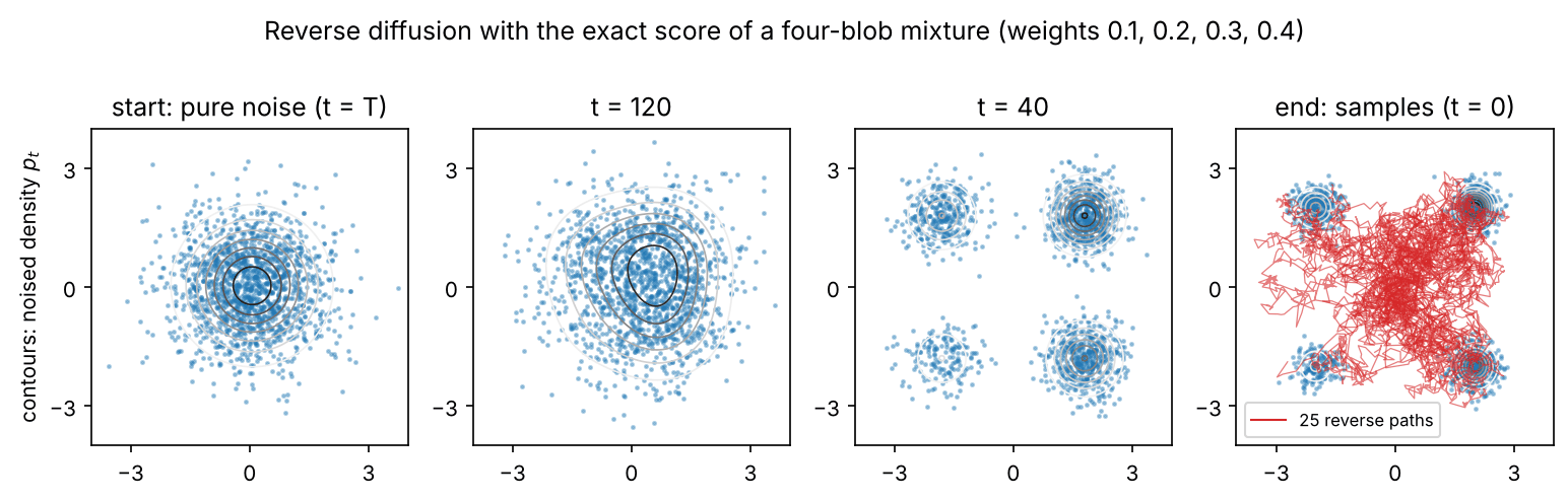
Code: diffusion with an exact score. Image-scale diffusion needs a trained network. On a 2-D toy we can skip the network: if the “image” distribution is a mixture of Gaussians, every noisy marginal is again a mixture of Gaussians, and its score has a closed form. The prior below has four blobs with weights 0.1, 0.2, 0.3, 0.4 and standard deviation 0.3.
Code · Python · 40 lines
import numpy as np

rng = np.random.default_rng(1)
mu = np.array([[-2.0, -2.0], [-2.0, 2.0], [2.0, -2.0], [2.0, 2.0]])  # a 2-D "image" prior:
w = np.array([0.1, 0.2, 0.3, 0.4])                                   # four Gaussian blobs
s2 = 0.3**2                                                          # each with variance s2 * I

T = 200
beta = np.linspace(1e-4, 0.05, T)
alpha = 1 - beta
abar = np.cumprod(alpha)

def score(x, ab):
    """Exact grad log p_t(x) of the noised mixture, plus responsibilities r."""
    m, v = np.sqrt(ab) * mu, ab * s2 + (1 - ab)            # component k at time t: N(m_k, v I)
    d2 = ((x[:, None, :] - m[None]) ** 2).sum(-1)         # (N, K) squared distances
    logr = np.log(w) - d2 / (2 * v)
    r = np.exp(logr - logr.max(1, keepdims=True)); r /= r.sum(1, keepdims=True)
    return (r[:, :, None] * (m[None] - x[:, None, :])).sum(1) / v, r

def x0_hat(x, ab):                                         # Tweedie: E[x_0 | x_t]
    return (x + (1 - ab) * score(x, ab)[0]) / np.sqrt(ab)

def ddpm_step(x, t, x0):
    """Sample x_{t-1} from the Gaussian q(x_{t-1} | x_t, x_0 = x0)."""
    ab_prev = abar[t - 1] if t > 0 else 1.0
    mean = (np.sqrt(ab_prev) * beta[t] * x0 + np.sqrt(alpha[t]) * (1 - ab_prev) * x) / (1 - abar[t])
    var = beta[t] * (1 - ab_prev) / (1 - abar[t])
    return mean + np.sqrt(var) * rng.standard_normal(x.shape)

x = rng.standard_normal((4000, 2))                         # start from pure noise
for t in reversed(range(T)):
    x = ddpm_step(x, t, x0_hat(x, abar[t]))
_, r = score(x, 1.0)
print("signal left at t=T:", round(abar[-1], 5))
print("fraction per blob :", np.bincount(r.argmax(1), minlength=4) / len(x), "(target", w, ")")
print("spread inside blob:", round(float(np.sqrt(((x - mu[r.argmax(1)]) ** 2).mean())), 3), "(target 0.3)")
# signal left at t=T: 0.00612
# fraction per blob : [0.09675 0.2005  0.3075  0.39525] (target [0.1 0.2 0.3 0.4] )
# spread inside blob: 0.283 (target 0.3)
The sampler reproduces the blob weights to within sampling error. The spread inside each blob is 0.283 instead of 0.3: with only 200 coarse steps the reverse process is slightly too narrow (with 1,000 smaller steps we measured 0.296). This is the first lesson about step count: fewer steps are cheaper and less exact. Figure 3 shows the particle cloud contracting from noise to the four blobs.
Route A: train a conditional diffusion restorer
The direct approach lets the denoiser see the input: train on pairs, so the sampler draws from an approximation of . SR3 [14] did this for super-resolution: the upsampled low-resolution image is given to the U-Net with the noisy image, and sampling refines pure noise step by step. In the paper’s human study on face super-resolution, raters were fooled by SR3 close to 50% of the time, against at most 34% for GAN baselines [14]. Palette [15] applied the recipe to colorization, inpainting, uncropping and JPEG restoration, and showed that one multi-task model can match task-specific ones.
Conditional models need pairs and new training for each family of degradations, but they cope with noise and with operators that are hard to write down (camera processing, compression). Starting from pure noise wastes steps re-creating what already contains; ResShift [16] instead builds a chain that moves between the high- and low-resolution images by shifting their residual, and reports competitive results with only 15 sampling steps.
Route B: zero-shot posterior sampling with a pretrained model
Plain version. Train one unconditional diffusion model on clean images. To restore, run its sampler as usual, but after every step check the current clean guess against the input and correct it a little. The model contributes “looks real”; the correction contributes “agrees with what we measured”.
Precise version. Apply the score identity of the previous section to the noisy variable :
where the first term is the pretrained model’s score and the second is the noisy likelihood: how well the noisy state explains . The first term we have. The second is the hard part, because depends on the clean image, and
averages the likelihood over all clean images that could have produced , which is intractable for an image-scale model. The methods differ mainly in how they approximate this term, and they all end up with the same loop (Figure 4): a prior step (one reverse-diffusion step with the pretrained model) and a data-consistency step (a gradient step, a projection or a closed-form correction toward ).
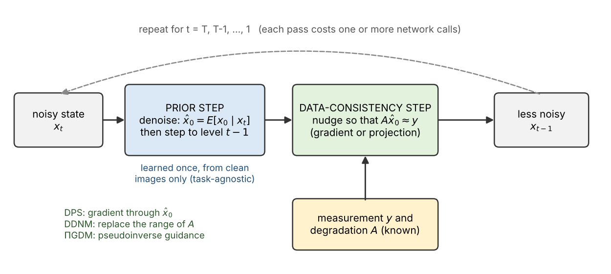
DPS (diffusion posterior sampling) [17] is the simplest to state. It replaces the average over by its mean, . With Gaussian noise this gives the data step
where is the result of the ordinary prior step and is a step size; the paper uses with a constant . The gradient passes through , so it needs backpropagation through the denoiser at every step. Because it never projects exactly onto the measurements, DPS also works with noisy and nonlinear degradations (the paper includes Poisson noise, Fourier phase retrieval and non-uniform deblurring).
The other members differ mainly in the data step:
- DDRM (denoising diffusion restoration models) [18] handles linear degradations in the coordinates of the degradation’s singular value decomposition, treating measured and unmeasured coordinates differently; no backpropagation, few steps.
- DDNM (denoising diffusion null-space model) [19] copies the part of that the measurement determines from the data, (with the pseudoinverse of a linear ), and keeps the model’s guess only in the part the measurement cannot see.
- ΠGDM (pseudoinverse-guided diffusion models) [20] builds its guidance from a pseudoinverse of the degradation and an explicit uncertainty for ; it backpropagates through the denoiser but not through the degradation, so it also covers non-differentiable measurements such as JPEG.
- DiffPIR [21] puts plug-and-play splitting (a data step and a denoiser step in turn, as described in DLCV 09) inside the diffusion sampler and reports good results with at most 100 network evaluations.
Optional: How the zero-shot diffusion samplers differ (in the Supplementary notes). The data step of each method, the range–null-space split and the SVD view, with a three-line check.
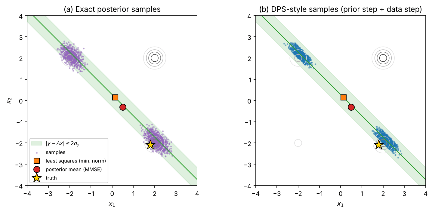
Code: a DPS-style sampler where the true posterior is known. We reuse the four-blob prior and observe one linear projection of the 2-D “image”, with and noise standard deviation . The blobs at and both have , so a measurement near 0 is genuinely ambiguous. Prior and likelihood are Gaussian within each blob, so the exact posterior is again a four-blob mixture and we can check the sampler against it. The Jacobian of is taken by finite differences, cheap in 2-D; at image scale this is the backpropagation step.
Code · Python · 43 lines
# Continues the previous snippet (same session): mu, w, s2, T, abar, x0_hat, ddpm_step.
rng = np.random.default_rng(3)
A = np.array([[1.0, 1.0]]) / np.sqrt(2)          # we only observe one projection of x
sig_y = 0.2
x_true = np.array([1.8, -2.1])
y = A @ x_true + sig_y * rng.standard_normal(1)

# Reference: the exact posterior of a Gaussian mixture under a linear-Gaussian measurement.
S = (A @ A.T)[0, 0] * s2 + sig_y**2               # variance of y within one blob
logpost = np.log(w) - (y - mu @ A.T)[:, 0] ** 2 / (2 * S)
post_w = np.exp(logpost - logpost.max()); post_w /= post_w.sum()
gain = s2 * A.T / S                               # Kalman gain, shape (2, 1)
post_mu = mu + (y - mu @ A.T) @ gain.T            # posterior mean inside each blob
post_cov = s2 * (np.eye(2) - gain @ A)
k = rng.choice(4, size=2000, p=post_w)
exact = post_mu[k] + rng.multivariate_normal(np.zeros(2), post_cov, size=2000)
mmse = post_w @ post_mu                           # posterior mean
least_sq = (np.linalg.pinv(A) @ y).ravel()        # minimum-norm solution of A x = y

def data_grad(x, ab, h=1e-4):
    """grad_x ||y - A x0_hat(x)||^2 through Tweedie's estimate (finite-difference Jacobian)."""
    J = np.stack([(x0_hat(x + h * e, ab) - x0_hat(x - h * e, ab)) / (2 * h) for e in np.eye(2)], -1)
    resid = y - x0_hat(x, ab) @ A.T                # (N, 1)
    return -2 * np.einsum("nij,ik,nk->nj", J, A.T, resid), np.abs(resid)

x = rng.standard_normal((2000, 2))
for t in reversed(range(T)):
    x_prior = ddpm_step(x, t, x0_hat(x, abar[t]))  # 1) prior step: one reverse-diffusion step
    g, res = data_grad(x, abar[t])
    x = x_prior - 0.1 / (res + 1e-8) * g           # 2) data-consistency step, DPS step size

blob = lambda pts: np.bincount(np.argmin(((pts[:, None] - mu) ** 2).sum(-1), 1), minlength=4) / len(pts)
print("least squares", least_sq.round(2), "| posterior mean", mmse.round(2), "| truth", x_true)
for name, pts in [("exact posterior", exact), ("DPS", x)]:
    print(f"{name:15s} blob shares {blob(pts)} | median |y - Ax| {np.median(np.abs(y - pts @ A.T)):.3f}"
          f" | mean sq. error {np.mean(((pts - x_true) ** 2).sum(1)):.2f}")
for name, est in [("least squares", least_sq), ("posterior mean", mmse)]:
    print(f"{name:15s} sq. error {np.sum((est - x_true) ** 2):.2f}")
# least squares [0.14 0.14] | posterior mean [ 0.5 -0.3] | truth [ 1.8 -2.1]
# exact posterior blob shares [0.    0.409 0.591 0.   ] | median |y - Ax| 0.122 | mean sq. error 12.97
# DPS             blob shares [0.     0.4055 0.5945 0.    ] | median |y - Ax| 0.100 | mean sq. error 13.09
# least squares   sq. error 7.77
# posterior mean  sq. error 4.93
Read the output with Figure 5:
- The least-squares solution and the posterior mean both lie between the two plausible blobs, where the prior is almost empty: the “blurry” answers of this toy. The posterior mean has the lowest squared error (4.93) because it hedges.
- The DPS-style samples fall in the two right blobs with shares 0.41 and 0.59, matching the exact posterior. Their mean squared error (13.09) is much higher, because about 40% of them land in the other blob: a confident, wrong answer. That is posterior sampling working as intended, and also the 2-D version of a hallucinated detail.
- DPS fits the measurement slightly more tightly than the true posterior (median residual 0.100 versus 0.122): it is an approximation, and its residual depends on the step size (Exercise 3). In high dimensions such deviations are much harder to see.
Optional: Chung et al., “Diffusion Posterior Sampling for General Noisy Inverse Problems” (in the Paper guides). What the paper approximates, what it measured and what to check in its tables.
Choosing between conditional and zero-shot
| Question | Conditional (SR3, Palette, ResShift) | Zero-shot (DPS, DDRM, DDNM, ΠGDM, DiffPIR) |
|---|---|---|
| Training | One model per family of degradations, on pairs | One unconditional model on clean images |
| Degradation at test time | Implicit; can be unknown if it was in training | Must be known (or estimated) and usually differentiable |
| Noise and real camera pipelines | Handled if they were in training | Handled only as far as the likelihood model allows |
| Cost per image | Tens to hundreds of steps, no backpropagation | Often hundreds of steps; DPS-type methods also backpropagate |
| Good fit | One task with plenty of training pairs | Known physics, new operators, no retraining |
A rough rule: if you can collect or synthesize pairs for exactly your degradation, train a conditional model (or a non-generative one). If the operator is known physics (a blur kernel, a sampling mask, a tomography projector) and retraining for every setting is impractical, zero-shot sampling is attractive.
Family 3: latent-diffusion and foundation-model restorers
Plain version. The strongest image generators are large text-to-image diffusion models trained on huge image collections. They know what grass, fabric and brick look like far better than any restoration dataset could teach. Recent real-world restorers keep such a model frozen (or almost frozen), add a small network that shows it the damaged image, and let it paint in the missing detail. The result can look stunning, and it can invent things.
Building on a pretrained text-to-image model
Latent diffusion [22] runs diffusion in the compressed latent space of an autoencoder instead of on pixels, which is what makes large text-to-image models affordable (ML 08). ControlNet [23] showed how to add a new image condition to such a model, which its authors describe as pretrained with billions of images, without damaging it: the pretrained model is locked, a trainable copy of its encoding layers receives the condition, and the two are joined by zero-initialized convolutions, so training starts from the unchanged model. Restoration methods adapt both ideas. StableSR [24] keeps the generator fixed and injects the low-quality image through a time-aware encoder, with a user-set scalar that trades quality for fidelity. DiffBIR [25] first removes the degradation with an ordinary restoration network and then regenerates lost detail with a ControlNet-style adapter, again with a tunable fidelity guidance. SUPIR [26] scales up the prior and the data (the paper describes 20 million high-resolution images with text annotations) and lets text prompts steer the restoration.
Fewer steps: from hundreds to one
Multi-step latent restorers are slow, and their random starting noise makes outputs vary from run to run. Distilled and re-designed models reduce both: SinSR [27], OSEDiff [28] and TSD-SR [30] restore in one step, and InvSR [29] in one to five, mostly by starting from the low-quality image instead of pure noise and by distilling a many-step teacher. The general distillation families (progressive, consistency, adversarial) are described in ML 08.
Optional: Latent and one-step restorers, method by method (in the Supplementary notes). What StableSR, DiffBIR, SUPIR, SinSR, OSEDiff, InvSR and TSD-SR each add.
Two consequences. First, a one-step restorer that starts from the input is nearly deterministic: it gives one plausible answer, like a GAN, rather than samples with the right spread. Second, step count is not the whole cost: a one-step model may have a larger network, and latent methods also pay for the autoencoder’s encoder and decoder at full resolution.
The hallucination problem
Plain version. A strong prior fills gaps with what is typical, not with what was there. Where the input says little, the output is mostly prior: it looks real, and nothing in the image tells you it was invented. Where it shows up:
- Text and symbols. Letters on signs, plates and documents are very specific: a small error changes the meaning. A generative restorer can produce clean, legible, wrong characters.
- Faces and identity. Face priors produce a face from the training distribution; for a specific person, a slightly different nose or eye is an identity change.
- Textures. Brick, fabric and foliage may be replaced by a different but equally plausible pattern.
- Latent decoders. The autoencoder of a latent restorer has its own reconstruction error; encode and decode a clean image to see what it alone changes, as ML 08 recommends.
- Medical and scientific images. A plausible structure that is not there, or a real lesion smoothed away, is a diagnostic error. Bhadra et al. [35] analyze this in tomographic reconstruction by splitting an estimate into the part determined by the measurements and a null-space part supplied by the prior, and define a hallucination map from it.
The null-space view explains the mechanism in one line, using the decomposition behind DDNM: for a linear , any estimate satisfies . Data consistency constrains only the first part. Everything in the second part, which is large when discards a lot, comes from the prior, so a perfectly data-consistent output can still be largely invented. Consistency with is necessary, never sufficient.
Measuring hallucination is itself a research topic. A recent study of generative super-resolution argues that hallucinated details are poorly captured both by fidelity metrics and by no-reference quality models, and proposes a “Hallucination Score” obtained by prompting a multimodal large language model, which its authors found to align closely with human judgments [36].
Family 4: flow matching and rectified flow restorers
Plain version. Flow matching learns a smooth “velocity field” that carries noise to images along nearly straight paths, so it needs few steps. For restoration, one can carry a blurry best guess to a realistic image, or plug a pretrained flow into the same prior-plus-data loop as diffusion.
Flow matching [31] and rectified flow [32] train a network to predict the velocity of a path between a simple distribution and the data distribution; samples come from integrating an ordinary differential equation, and straight paths need few integration steps (ML 08). Two verified restoration uses:
- PMRF (posterior-mean rectified flow) [33] targets the point of the perception–distortion section directly: the estimator with the lowest MSE among those whose outputs are distributed like real images. Following a theoretical result the paper cites, it first predicts the posterior mean (an ordinary MMSE network) and then transports that blurry estimate to a realistic image with a rectified flow model that approximates the optimal transport map. This is a clean way to think about the whole chapter: first get the best average, then move it as little as possible to make it look real.
- PnP-Flow [34] defines a time-dependent denoiser from a pretrained flow-matching model and alternates gradient steps on the data-fidelity term, reprojections onto the learned flow path, and denoising: the loop of Figure 4 with a flow instead of a diffusion model, avoiding backpropagation through the ODE.
Evaluating generative restoration
Plain version. Ask four separate questions: is the output close to the truth (when you have it)? Does it look real? Does it agree with the input? And how much does it change when you run it again? One number cannot answer all four, and a pretty picture answers none of them.
The metric definitions are in DLCV 09. For a generative restorer, use them as follows.
- Fidelity, when a reference exists. PSNR and SSIM [39] (low distortion), LPIPS [38] (perceptual distance to the reference). An exact, conditionally independent posterior sample has twice the MMSE estimator’s expected squared error under the same data model [1]. This gives about a 3 dB gap only when PSNR is computed from those expected MSEs, not necessarily when per-image PSNR is averaged. A learned generator and a trained regression baseline need not satisfy these ideal assumptions. Measure their actual trade-off; a lower PSNR alone is not evidence of greater realism.
- Realism. No-reference metrics such as NIQE [41], MUSIQ [42] and CLIP-IQA [43] score single images; FID [40] compares Gaussian approximations to feature distributions of output and real-image sets. It is a practical distributional proxy, not an exact distance between the full image distributions and , and it needs many images. No-reference metrics can be gamed by adding texture, so never use them alone.
- Consistency with the input. Re-apply the degradation and compare: should be about the noise level. This needs no reference and catches outputs that ignore the input. It cannot catch null-space hallucinations (previous section).
- Stochasticity. A sampler gives a distribution of outputs. Report it.
Reporting several samples. The snippet continues the step-edge toy: one test input, eight restorations per run, and three runs with different seeds, as three users of the same method would see.
Code · Python · 31 lines
# Recreate the step-edge toy: the intervening DPS example uses a different A.
import numpy as np
from scipy.ndimage import gaussian_filter1d
n, factor, sigma = 64, 8, 0.2
positions = np.arange(8, 56)
X = (np.arange(n)[None, :] >= positions[:, None]).astype(float)
A = lambda x: gaussian_filter1d(x, 3.0, axis=-1, mode="nearest")[..., ::factor]
AX = A(X)

def posterior(y):
    logp = -np.sum((y - AX)**2, axis=1) / (2 * sigma**2)
    p = np.exp(logp - logp.max())
    return p / p.sum()

rng = np.random.default_rng(5)
x = X[20]                                                   # a test signal: edge at pixel 28
y = A(x) + sigma * rng.standard_normal(n // factor)
p = posterior(y)
for seed in range(3):                                       # three "users" with different seeds
    r = np.random.default_rng(seed)
    S = X[r.choice(len(positions), size=8, p=p)]            # 8 restorations of the same input
    err = ((S - x) ** 2).mean(axis=1)
    print(f"seed {seed}: MSE mean {err.mean():.4f} ± {err.std():.4f} | best of 8 {err.min():.4f}"
          f" | edges at {sorted(set(np.argmax(S, axis=1).tolist()))}")
S = X[rng.choice(len(positions), size=200, p=p)]
std = S.std(axis=0)                                         # per-pixel spread across samples
print("pixels with std > 0.1:", np.flatnonzero(std > 0.1), "| true edge at", np.argmax(x))
# seed 0: MSE mean 0.0273 ± 0.0268 | best of 8 0.0000 | edges at [23, 24, 26, 27, 28, 29]
# seed 1: MSE mean 0.0273 ± 0.0103 | best of 8 0.0156 | edges at [25, 26, 27, 29, 30]
# seed 2: MSE mean 0.0293 ± 0.0213 | best of 8 0.0000 | edges at [24, 25, 26, 27, 28]
# pixels with std > 0.1: [22 23 24 25 26 27 28 29 30] | true edge at 28
Three lessons, each with a reporting rule:
- The spread is as large as the mean. On one input, the per-sample MSE varies by about as much as its average. Report the mean and the spread over samples (and over seeds), not one sample.
- “Best of K” is an oracle. Picking the sample closest to the ground truth gives an MSE of zero for two of the three seeds, a number no user can obtain because users do not have the ground truth. If a paper reports best-of-K, it must say so, and it should not be compared with single-sample results. (DPS, for example, reports the best of four samples for phase retrieval, following common practice for that problem, and says so [17].)
- Sample spread is a diagnostic, not a calibrated error map. The per-pixel standard deviation over 200 samples is large around the edge (pixels 22 to 30) in this exact-posterior toy. A learned sampler can instead repeat the same wrong detail, giving low spread despite high error; additional samples also cost computation. Angelopoulos et al. [37] calibrate image-valued prediction sets on held-out data: with a chosen confidence over calibration, they bound the expected fraction of uncovered pixels on fresh images from the same distribution. That is not a guarantee for every pixel of every individual image, nor a guarantee under arbitrary distribution shift.
Compute. Report the number of network evaluations (NFE), including guidance and any extra passes, the resolution, the hardware and wall-clock time, and for latent methods the autoencoder’s cost. As a concrete anchor, the DPS paper reports about 95 seconds per FFHQ image and about 600 seconds per ImageNet image, each with 1,000 network evaluations on one RTX 2080 Ti GPU [17]. Distilled one-step restorers cut the step count to one, but compare full pipelines, not step counts.
A minimal honest report: PSNR/SSIM and LPIPS on references; two or three no-reference metrics from different families, plus FID on a large enough set; the re-degradation residual; mean and spread over samples and seeds; NFE and time; a user study for headline claims; and a gallery that includes failures, not only the best-looking results.
Failure modes and when NOT to use generative restoration
Plain version. Generative restoration is the right tool when the goal is a pleasant, plausible picture. It is the wrong tool when the picture will be used as evidence.
Typical failure modes.
- Hallucinated specifics: text, digits, faces, small objects, medical findings (see the hallucination section).
- Ignoring the input: weak data consistency, especially with strong guidance toward the prior or a prompt, gives realistic images of a slightly different scene; color shifts are a known issue of diffusion super-resolution [46].
- Mismatch between assumed and real degradation: zero-shot methods need the right . A wrong blur kernel or noise level is propagated by the data step, and the prior then makes the wrong answer look convincing.
- Out-of-distribution inputs: a prior trained on faces or natural photos pulls microscopy, satellite or medical images toward the wrong “typical” appearance, and faces unlike the training data toward the typical face (the bias discussed for PULSE [7]).
- Instability across runs and sizes: different seeds give different details, and models trained at a fixed size need special handling for larger images (StableSR’s progressive aggregation sampling is one answer [24]).
- Cost: hundreds of network calls per image, or a very large one-step network.
When not to use it, or to use it only with explicit labeling and uncertainty:
- Evidence and measurement: forensic, legal, journalistic and surveillance use, license plates, documents to be read, anything where a person will act on a detail. Prefer an MMSE restorer (smooth, but it does not commit to specifics) or show a set of samples with an uncertainty map.
- Medicine and science: diagnosis, quantification and any downstream measurement. Use methods validated for the task, with hallucination analysis such as [35], and keep the measured data visible.
- Mild degradations: when the posterior is narrow (light noise, super-resolution of a clean image), a regression network already gives a sharp answer, faster and with less risk.
- Pipelines that feed another algorithm (detection, OCR, measurement): restoration should be judged by the downstream task; invented detail can create false detections.
A short decision rule: if a wrong but realistic detail is worse than a blurry region, do not use a generative restorer without uncertainty reporting.
Modern view
Survey papers.
- Li et al., “Diffusion Models for Image Restoration and Enhancement: A Comprehensive Survey” (IJCV 2025) [44]. Splits diffusion restoration into supervised methods (grouped by how they condition the sampler) and zero-shot methods (projection, decomposition and posterior estimation), adds blind and real-world restoration, and compares methods on several tasks. Takeaway: the best perceptual quality, with sampling cost, model size, real-world degradations and evaluation as the main obstacles.
- Daras et al., “A Survey on Diffusion Models for Inverse Problems” (arXiv 2024) [45]. Covers methods that use a pretrained diffusion model without further training, in four families by how they treat the measurement term: explicit approximations of (DPS, ΠGDM and the DDRM family among them), variational inference, CSGM-type latent optimization and asymptotically exact Monte Carlo methods; a second taxonomy sorts them by how consistency is enforced (gradients, projections, sampling, optimization). Takeaway: many seemingly different methods compute a measurement error and “lift” it back to image space in different ways, and the field lacks a standard benchmark of quality versus compute.
- Moser et al., “Diffusion Models, Image Super-Resolution, and Everything: A Survey” (IEEE TNNLS 2025) [46]. Concentrates on super-resolution: foundations, input domains (pixel or latent), conditioning, guidance, corruption spaces and zero-shot methods. Takeaway: diffusion closed much of the gap to human preference, while computational cost, comparability between papers, explainability and color shifts are open.
- Xia et al., “GAN Inversion: A Survey” (IEEE TPAMI 2023) [47]. Reviews how images are mapped back into a pretrained GAN’s latent space and how this supports restoration and editing. Takeaway: the GAN-prior methods of Family 1 are special cases of inversion, and their limits are the generator’s coverage and the inversion’s cost.
Optional: Li et al., “Diffusion Models for Image Restoration and Enhancement: A Comprehensive Survey” (in the Paper guides). How to use the survey’s taxonomy and comparison tables.
State of the art, 2023–2026.
- Pretrained text-to-image models became the default prior for real-world restoration, connected through adapters (StableSR, DiffBIR, SUPIR), with explicit fidelity knobs because uncontrolled generation drifts from the input.
- Step counts fell from hundreds to one through residual-shifting chains, distillation and inversion (ResShift, SinSR, OSEDiff, InvSR, TSD-SR). One-step models trade the posterior’s spread for speed and repeatability.
- Zero-shot posterior sampling matured into a family with shared structure (DPS, DDRM, DDNM, ΠGDM, DiffPIR) and was extended to flows (PnP-Flow), with surveys that unify the approximations [45].
- Theory re-entered practice: the perception–distortion bound now guides method design directly, as in PMRF’s “posterior mean, then transport” [33].
- Hallucination started to be measured, not only mentioned, for example with dedicated scores [36].
Open problems.
- Measuring faithfulness: no accepted metric says “sharp and correct”. Fidelity metrics penalize all detail; no-reference metrics reward invented detail.
- True posterior sampling at image scale: zero-shot methods are approximate (our toy shows a small bias even in 2-D), and few-step models give little diversity. Calibrated uncertainty for high-resolution images is largely open.
- Unknown degradations: zero-shot methods need ; supervised ones need the right training distribution.
- Cost: high-resolution and video restoration with large priors remain expensive.
- Responsible use: domain shift, demographic bias of face priors and the labeling of generated content are unsolved in practice.
Optional: DDNM, DPS, BlindDPS (in the Paper guides). Compare a known noiseless linear operator, noisy likelihood guidance and a jointly estimated unknown operator.
Key takeaways
- The optimal squared-error estimate is the conditional mean; averaging ambiguous structures can blur them.
- A plausible generated detail may differ from the original scene.
- Perception–distortion bounds concern ideal distributions and estimators [1]; learned generators do not automatically satisfy them.
- Distinguish task-trained conditional models from pretrained priors coupled to measurement constraints.
- Input consistency cannot detect inventions in unobserved components; fewer sampling steps do not remove this ambiguity.
- Report fidelity, realism, consistency, seeds and full cost; never hide best-of-many selection.
- Choose conservative restoration when a realistic wrong detail would undermine the application.
Exercises
- The factor of two, by hand. In the step-edge toy, suppose that for one input the posterior puts probability 0.5 on an edge at pixel 30 and 0.5 on an edge at pixel 32, and the truth is at 30. Compute the MSE (per pixel, over 64 pixels) of the posterior mean and the expected MSE of a posterior sample. Is the ratio two? Explain why the factor of two in the theorem is an average over inputs, not a guarantee for each input.
Hint
The two candidates differ only at pixels 30 and 31. The mean is 0.5 there, so its MSE is ; a sample is right with probability 0.5 and wrong by 1 at two pixels otherwise, so its expected MSE is : a ratio of two. If instead the posterior put 0.9 on the wrong position, the ratio for this truth would be . The theorem averages over and jointly, where the truth itself is distributed like the posterior.
- Walking the trade-off. Using the first snippet, compute MSE and W1 for (a) the posterior mean plus Gaussian noise of standard deviation 0.1, (b) the posterior median edge position (choose the position where the posterior’s cumulative probability first exceeds 0.5), and (c) the posterior mode. Place them on Figure 2’s plane. Which are near the posterior-sample point?
Hint
Adding noise does not create edges: in our run the largest step was only 0.40, W1 grew to about 0.095 (noise creates many unrealistic in-between values) and the MSE grew to 0.0274, so (a) moves away from both goals. The median and the mode are single real edges, so their W1 is near zero like a sample’s (0.0009 and 0.0011 in our run), and their MSE (0.0245 and 0.0259) is below a random sample’s (0.0338) because they never pick an unlikely position. They are deterministic, though: they do not reproduce the posterior’s spread, which a set-level metric could detect (all outputs for similar inputs agree).
- DPS step size. In the DPS-style snippet, replace the constant 0.1 in the data step by 0.02, 0.5 and 2.0. For each, report the blob shares, the median residual and the mean squared error, and compare with the exact posterior. Then replace the normalized step by an unnormalized step . What do you conclude about how DPS’s step size relates to the noise level ?
Hint
With the normalized step, each data step has roughly the same length whatever the residual, so the final median residual settles near the constant itself (in our runs 0.021, 0.100, 0.496 and 1.994 for 0.02, 0.1, 0.5 and 2.0). Large values leave residuals far above the noise level and distort the blob shares (0.24 and 0.76 at 2.0, against 0.41 and 0.59 exactly); at 0.02 about 1% of the samples ended in a blob the measurement rules out, because the early corrections were too weak. The unnormalized step gave a median residual of 0.007, far tighter than the noise level allows. Neither choice is tied to the way an exact posterior is: the step size is a tuned hyperparameter, one reason DPS is an approximation.
- Steps and accuracy. In the diffusion snippet, run the sampler with (and
beta = np.linspace(1e-4, 0.2, T)) and with (andnp.linspace(1e-4, 0.01, T)). Record the spread inside each blob. Relate the result to the cost discussion and to why distilled one-step restorers are trained rather than obtained by simply using fewer steps.
Hint
In our runs the spread was about 0.263 for 50 steps, 0.283 for 200 and 0.296 for 1,000 (target 0.3): coarse steps make the reverse process too narrow even with the exact score. A one-step model cannot get its accuracy by taking one huge step of the same sampler; it must be trained (distilled or built differently) to jump correctly.
- Null-space hallucination. Take a 1-D signal of length 16 and = average of consecutive pairs (an matrix). Compute and verify that is a projection (). Construct two different signals with exactly the same measurement , one smooth and one with a sharp checkerboard pattern. Which one would a generative prior of natural signals pick, and which part of each signal is “invented”?
Hint
The null space of pair-averaging contains every pattern that alternates sign within a pair, with any amplitude per pair; adding it to a smooth signal leaves unchanged. The within-pair differences, , are invisible to the data and supplied entirely by the prior: a smooth-signal prior picks small ones, a texture prior may add some. This is the hallucination-map idea of [35].
- Design an evaluation. You must decide whether a one-step latent-diffusion restorer can replace an MSE-trained network for restoring scanned archival documents. Write the evaluation protocol: data, metrics, number of samples and seeds, a check for hallucinated characters, compute measurements, and a decision rule.
Hint
Use real scans with references where possible (rescan at high resolution) plus synthetic degradations of clean documents. Report PSNR/SSIM/LPIPS, a no-reference metric, and, crucially, an OCR character error rate against the true text for both methods and for several seeds; also report how often two seeds disagree on a character (an uncertainty signal). Include NFE, time and memory including the autoencoder. Decide by the task: if the generative model raises character errors or changes characters between seeds, keep the MSE network for reading and use the generative one only for display, clearly labeled.
References
- Y. Blau and T. Michaeli, “The Perception-Distortion Tradeoff,” in Proc. IEEE/CVF CVPR, 2018, pp. 6228–6237 (extended version on arXiv). doi · arXiv
- C. Ledig, L. Theis, F. Huszár, J. Caballero, A. Cunningham, A. Acosta, A. Aitken, A. Tejani, J. Totz, Z. Wang and W. Shi, “Photo-Realistic Single Image Super-Resolution Using a Generative Adversarial Network,” in Proc. IEEE CVPR, 2017, pp. 105–114. doi · arXiv
- J. Johnson, A. Alahi and L. Fei-Fei, “Perceptual Losses for Real-Time Style Transfer and Super-Resolution,” in Proc. ECCV, 2016, pp. 694–711. doi · arXiv
- X. Wang, K. Yu, S. Wu, J. Gu, Y. Liu, C. Dong, Y. Qiao and C. C. Loy, “ESRGAN: Enhanced Super-Resolution Generative Adversarial Networks,” in Proc. ECCV Workshops, 2018 (LNCS, 2019), pp. 63–79. doi · arXiv
- X. Wang, L. Xie, C. Dong and Y. Shan, “Real-ESRGAN: Training Real-World Blind Super-Resolution with Pure Synthetic Data,” in Proc. IEEE/CVF ICCV Workshops, 2021, pp. 1905–1914. doi · arXiv
- T. Karras, S. Laine and T. Aila, “A Style-Based Generator Architecture for Generative Adversarial Networks,” in Proc. IEEE/CVF CVPR, 2019, pp. 4396–4405. doi · arXiv
- S. Menon, A. Damian, S. Hu, N. Ravi and C. Rudin, “PULSE: Self-Supervised Photo Upsampling via Latent Space Exploration of Generative Models,” in Proc. IEEE/CVF CVPR, 2020, pp. 2434–2442. doi · arXiv
- K. C. K. Chan, X. Wang, X. Xu, J. Gu and C. C. Loy, “GLEAN: Generative Latent Bank for Large-Factor Image Super-Resolution,” in Proc. IEEE/CVF CVPR, 2021, pp. 14240–14249. doi · arXiv
- X. Wang, Y. Li, H. Zhang and Y. Shan, “Towards Real-World Blind Face Restoration with Generative Facial Prior,” in Proc. IEEE/CVF CVPR, 2021, pp. 9164–9174. doi · arXiv
- S. Zhou, K. C. K. Chan, C. Li and C. C. Loy, “Towards Robust Blind Face Restoration with Codebook Lookup Transformer,” in Proc. NeurIPS, vol. 35, 2022, pp. 30599–30611. doi · arXiv
- J. Ho, A. Jain and P. Abbeel, “Denoising Diffusion Probabilistic Models,” in Proc. NeurIPS, 2020. proceedings · arXiv
- Y. Song, J. Sohl-Dickstein, D. P. Kingma, A. Kumar, S. Ermon and B. Poole, “Score-Based Generative Modeling through Stochastic Differential Equations,” in Proc. ICLR, 2021. arXiv
- B. Efron, “Tweedie’s Formula and Selection Bias,” Journal of the American Statistical Association, vol. 106, no. 496, pp. 1602–1614, 2011. doi
- C. Saharia, J. Ho, W. Chan, T. Salimans, D. J. Fleet and M. Norouzi, “Image Super-Resolution via Iterative Refinement,” IEEE TPAMI, 2022 (early access). doi · arXiv
- C. Saharia, W. Chan, H. Chang, C. Lee, J. Ho, T. Salimans, D. Fleet and M. Norouzi, “Palette: Image-to-Image Diffusion Models,” in Proc. ACM SIGGRAPH Conference, 2022, pp. 1–10. doi · arXiv
- Z. Yue, J. Wang and C. C. Loy, “ResShift: Efficient Diffusion Model for Image Super-resolution by Residual Shifting,” in Proc. NeurIPS, vol. 36, 2023, pp. 13294–13307. doi · arXiv
- H. Chung, J. Kim, M. T. McCann, M. L. Klasky and J. C. Ye, “Diffusion Posterior Sampling for General Noisy Inverse Problems,” in Proc. ICLR, 2023. arXiv
- B. Kawar, M. Elad, S. Ermon and J. Song, “Denoising Diffusion Restoration Models,” in Proc. NeurIPS, vol. 35, 2022, pp. 23593–23606. doi · arXiv
- Y. Wang, J. Yu and J. Zhang, “Zero-Shot Image Restoration Using Denoising Diffusion Null-Space Model,” in Proc. ICLR, 2023. arXiv
- J. Song, A. Vahdat, M. Mardani and J. Kautz, “Pseudoinverse-Guided Diffusion Models for Inverse Problems,” in Proc. ICLR, 2023. ICLR page
- Y. Zhu, K. Zhang, J. Liang, J. Cao, B. Wen, R. Timofte and L. Van Gool, “Denoising Diffusion Models for Plug-and-Play Image Restoration,” in Proc. IEEE/CVF CVPR Workshops, 2023, pp. 1219–1229. doi · arXiv
- R. Rombach, A. Blattmann, D. Lorenz, P. Esser and B. Ommer, “High-Resolution Image Synthesis with Latent Diffusion Models,” in Proc. IEEE/CVF CVPR, 2022, pp. 10674–10685. doi · arXiv
- L. Zhang, A. Rao and M. Agrawala, “Adding Conditional Control to Text-to-Image Diffusion Models,” in Proc. IEEE/CVF ICCV, 2023, pp. 3813–3824. doi · arXiv
- J. Wang, Z. Yue, S. Zhou, K. C. K. Chan and C. C. Loy, “Exploiting Diffusion Prior for Real-World Image Super-Resolution,” International Journal of Computer Vision, vol. 132, no. 12, pp. 5929–5949, 2024. doi · arXiv
- X. Lin, J. He, Z. Chen, Z. Lyu, B. Dai, F. Yu, Y. Qiao, W. Ouyang and C. Dong, “DiffBIR: Toward Blind Image Restoration with Generative Diffusion Prior,” in Proc. ECCV, 2024 (LNCS), pp. 430–448. doi · arXiv
- F. Yu, J. Gu, Z. Li, J. Hu, X. Kong, X. Wang, J. He, Y. Qiao and C. Dong, “Scaling Up to Excellence: Practicing Model Scaling for Photo-Realistic Image Restoration In the Wild,” in Proc. IEEE/CVF CVPR, 2024, pp. 25669–25680. doi · arXiv
- Y. Wang, W. Yang, X. Chen, Y. Wang, L. Guo, L.-P. Chau, Z. Liu, Y. Qiao, A. C. Kot and B. Wen, “SinSR: Diffusion-Based Image Super-Resolution in a Single Step,” in Proc. IEEE/CVF CVPR, 2024, pp. 25796–25805. doi · arXiv
- R. Wu, L. Sun, Z. Ma and L. Zhang, “One-Step Effective Diffusion Network for Real-World Image Super-Resolution,” in Proc. NeurIPS, vol. 37, 2024, pp. 92529–92553. doi · arXiv
- Z. Yue, K. Liao and C. C. Loy, “Arbitrary-steps Image Super-resolution via Diffusion Inversion,” in Proc. IEEE/CVF CVPR, 2025, pp. 23153–23163. doi · arXiv
- L. Dong, Q. Fan, Y. Guo, Z. Wang, Q. Zhang, J. Chen, Y. Luo and C. Zou, “TSD-SR: One-Step Diffusion with Target Score Distillation for Real-World Image Super-Resolution,” in Proc. IEEE/CVF CVPR, 2025, pp. 23174–23184. doi · arXiv
- Y. Lipman, R. T. Q. Chen, H. Ben-Hamu, M. Nickel and M. Le, “Flow Matching for Generative Modeling,” in Proc. ICLR, 2023. arXiv
- X. Liu, C. Gong and Q. Liu, “Flow Straight and Fast: Learning to Generate and Transfer Data with Rectified Flow,” in Proc. ICLR, 2023. arXiv
- G. Ohayon, T. Michaeli and M. Elad, “Posterior-Mean Rectified Flow: Towards Minimum MSE Photo-Realistic Image Restoration,” in Proc. ICLR, 2025. arXiv
- S. Martin, A. Gagneux, P. Hagemann and G. Steidl, “PnP-Flow: Plug-and-Play Image Restoration with Flow Matching,” in Proc. ICLR, 2025. arXiv
- S. Bhadra, V. A. Kelkar, F. J. Brooks and M. A. Anastasio, “On Hallucinations in Tomographic Image Reconstruction,” IEEE Transactions on Medical Imaging, vol. 40, no. 11, pp. 3249–3260, 2021. doi · arXiv
- W. Ren, R. Goyal, Z. Hu, T. T. Aumentado-Armstrong, I. Mohomed and A. Levinshtein, “Hallucination Score: Towards Mitigating Hallucinations in Generative Image Super-Resolution,” arXiv:2507.14367, 2025. arXiv
- A. N. Angelopoulos, A. P. Kohli, S. Bates, M. I. Jordan, J. Malik, T. Alshaabi, S. Upadhyayula and Y. Romano, “Image-to-Image Regression with Distribution-Free Uncertainty Quantification and Applications in Imaging,” in Proc. ICML, PMLR 162, 2022. proceedings · arXiv
- R. Zhang, P. Isola, A. A. Efros, E. Shechtman and O. Wang, “The Unreasonable Effectiveness of Deep Features as a Perceptual Metric,” in Proc. IEEE/CVF CVPR, 2018, pp. 586–595. doi · arXiv
- Z. Wang, A. C. Bovik, H. R. Sheikh and E. P. Simoncelli, “Image Quality Assessment: From Error Visibility to Structural Similarity,” IEEE Transactions on Image Processing, vol. 13, no. 4, pp. 600–612, 2004. doi
- M. Heusel, H. Ramsauer, T. Unterthiner, B. Nessler and S. Hochreiter, “GANs Trained by a Two Time-Scale Update Rule Converge to a Local Nash Equilibrium,” in Proc. NeurIPS (NIPS), 2017. arXiv
- A. Mittal, R. Soundararajan and A. C. Bovik, “Making a ‘Completely Blind’ Image Quality Analyzer,” IEEE Signal Processing Letters, vol. 20, no. 3, pp. 209–212, 2013. doi
- J. Ke, Q. Wang, Y. Wang, P. Milanfar and F. Yang, “MUSIQ: Multi-scale Image Quality Transformer,” in Proc. IEEE/CVF ICCV, 2021, pp. 5128–5137. doi · arXiv
- J. Wang, K. C. K. Chan and C. C. Loy, “Exploring CLIP for Assessing the Look and Feel of Images,” in Proc. AAAI, vol. 37, no. 2, 2023, pp. 2555–2563. doi · arXiv
- X. Li, Y. Ren, X. Jin, C. Lan, X. Wang, W. Zeng, X. Wang and Z. Chen, “Diffusion Models for Image Restoration and Enhancement: A Comprehensive Survey,” International Journal of Computer Vision, vol. 133, no. 11, pp. 8078–8108, 2025. doi · arXiv
- G. Daras, H. Chung, C.-H. Lai, Y. Mitsufuji, J. C. Ye, P. Milanfar, A. G. Dimakis and M. Delbracio, “A Survey on Diffusion Models for Inverse Problems,” arXiv:2410.00083, 2024. arXiv
- B. B. Moser, A. S. Shanbhag, F. Raue, S. Frolov, S. Palacio and A. Dengel, “Diffusion Models, Image Super-Resolution, and Everything: A Survey,” IEEE Transactions on Neural Networks and Learning Systems, vol. 36, no. 7, pp. 11793–11813, 2025. doi · arXiv
- W. Xia, Y. Zhang, Y. Yang, J.-H. Xue, B. Zhou and M.-H. Yang, “GAN Inversion: A Survey,” IEEE TPAMI, vol. 45, no. 3, pp. 3121–3138, 2023. doi · arXiv
- Y. Song and S. Ermon, “Generative Modeling by Estimating Gradients of the Data Distribution,” in Proc. NeurIPS, 2019. arXiv
- H. Chung, J. Kim, S. Kim and J. C. Ye, “Parallel Diffusion Models of Operator and Image for Blind Inverse Problems,” in Proc. IEEE/CVF CVPR, 2023, pp. 6059–6069. paper
Check your understanding
This tutorial has 6 exercises. Can you solve them without opening the hints?
Go to the exercises ↑Next DLCV 09C · Low-Light Image Enhancement · 42 min