NLP 07 · Attention Mechanism and Transformers
Needs: NLP 06 · Sequence Labeling with RNNs (POS Tagging, Information Extraction)
Navigate: this page and this track: Navigate: this page and this track
On this page
- What you’ll learn1 min
- The big picture1 min
- 1. The encoder–decoder bottleneck1 min
- 2. Additive attention (Bahdanau)1 min
- 3. Multiplicative attention (Luong)1 min
- 4. Queries, keys and values: from alignment to self-attention1 min
- 5. Scaled dot-product attention3 min
- 6. Multi-head attention1 min
- 7. Self-attention and cross-attention1 min
- 8. Masks: padding and causal3 min
- 9. Position: telling attention where tokens are2 min
- 10. The Transformer encoder and decoder blocks3 min
- 11. Cost and long-context variants2 min
- Modern view2 min
- Key takeaways1 min
- Exercises2 min
- Paper guides
- References
Natural Language Processing
Explore this chapter 1 interactive experiment
Compare bidirectional and causal attention using the same query, keys and values.
What you’ll learn
- Why squeezing a whole source sentence into one vector limits an encoder–decoder, and how attention removes that bottleneck.
- The additive (Bahdanau) and multiplicative (Luong) attention equations, and how they generalize to queries, keys and values.
- Scaled dot-product attention, multi-head attention, and the difference between self-attention and cross-attention.
- How padding masks and causal masks encode what each position is allowed to read, and how to test that they work.
- Why attention needs position information, and the main ways to supply it.
- How Transformer encoder and decoder blocks are assembled, what they cost, and which variants target long contexts.
The big picture
Recurrent networks (NLP 05) read a sentence one token at a time and carry a running summary. That summary has a fixed size, whether the sentence has five words or fifty. Attention changes the access pattern: instead of relying on one summary, a position can look back at every stored representation and decide which ones matter for the prediction it is making now. The Transformer takes this idea to its conclusion and builds both the encoder and the decoder out of attention and small per-token networks, with no recurrence at all.
Three decisions organize this chapter, and they are worth keeping separate. The scoring rule decides how strongly one position matches another. The visibility rule, expressed as a mask, decides which positions may be read at all. The position rule decides how word order enters a computation that would otherwise ignore it. A change to one does not fix a mistake in another: a better scoring function cannot repair a mask that leaks future tokens.
Hagiwara’s Chapter 8 develops attention and Transformers for practical NLP [1]. This chapter adds the derivations, connects them to the original papers, and builds every mechanism in small CPU examples. ML 05 treats the same machinery from the vision side, with the full positional-encoding math; NLP 08 uses it to build a translation model.
1. The encoder–decoder bottleneck
Plain version. A sequence-to-sequence model has an encoder that reads the source and a decoder that writes the target. If the only bridge between them is one vector, every detail the decoder needs must fit through that vector.
The recurrent encoder–decoder models of Sutskever, Vinyals and Le [2] and Cho et al. [3] read a source sequence with an encoder RNN and pass its final state to the decoder:
Here is the encoder state after reading source token ; is the source length; is the single context vector; is the decoder state at target step ; is the previous target token; is the target prefix; and are recurrent update functions such as LSTM or GRU cells; and is an output layer followed by a softmax over the target vocabulary. ML 04 derives these cells and trains such a model.
The vector has the same dimension for every input. A ten-word sentence and a sixty-word paragraph must both be compressed into it before the first target word is produced. Bahdanau, Cho and Bengio named this fixed-length vector as a likely bottleneck for basic encoder–decoders and proposed letting the decoder search the source for the relevant parts instead [4]. Sutskever et al. also reported that reversing the source order helped their LSTM model, which is consistent with the same diagnosis: shortening the path between the first source words and the first target words made them easier to use [2].
The bottleneck is about information flow, not only capacity. Even a large must be computed before the decoder knows which source detail it will need at step . Attention postpones that choice: the encoder keeps one vector per source token, and the decoder chooses a different mixture of them at every step.
2. Additive attention (Bahdanau)
Plain version. At each target step, score every source position against what the decoder currently needs, turn the scores into weights that sum to one, and take the weighted average of the encoder states.
Bahdanau et al. [4] keep all encoder states (from a bidirectional encoder) and compute, for target step ,
Here is the previous decoder state; is the encoder state for source position ; , and are learned matrices and a learned vector; is the alignment score; is the attention weight, nonnegative and summing to one over ; and is the step-specific context vector, which the decoder uses together with its own state to predict . The notation matches ML 04. Because the score passes the two vectors through a small feedforward layer before comparing them, this form is called additive attention.
Two consequences matter for NLP. First, the decoder now has a direct path to every source token, so the information about the first source word no longer has to survive many recurrent updates. Second, the weights form a soft alignment between target and source positions, which can be plotted and inspected. That inspection is a diagnostic, not a guarantee: as discussed below, a large weight shows where the computation read from, not why the final prediction is correct.
3. Multiplicative attention (Luong)
Plain version. Replace the small scoring network by a dot product, possibly through one learned matrix. It is cheaper and turns attention into matrix multiplication.
Luong, Pham and Manning [5] compared several scoring functions for a global attention model that attends to all source states. They score the current decoder state (rather than the previous one) against each source state :
Here is the top-layer decoder state at target step ; is the encoder state at source position ; is a learned matrix; and is the attention weight. Their third option, concat, scores the concatenation with a feedforward layer, as in additive attention. The context vector is combined with the decoder state into an attentional hidden state, which feeds the output softmax:
Here is vector concatenation and , are learned matrices. Luong et al. also proposed local attention, which first predicts an aligned source position and attends only to a window around it, and input feeding, which passes into the next decoder step so the model knows its earlier alignment decisions [5].
The “general” score is the bridge to Transformers. Write and ; then the score is just . Once every score is a dot product between a query and a key, a whole table of scores is a single matrix product, which is what modern hardware does best.
4. Queries, keys and values: from alignment to self-attention
Plain version. Generalize the decoder state into a query (what this position is looking for), the source states into keys (what each position offers for matching) and values (what each position passes on if it is read). Attention then works between any two sets of vectors, including a sequence and itself.
In additive and multiplicative attention, the same encoder state is used both for matching and for the weighted sum. The Transformer separates these roles with three learned projections [6]. If the queries come from the decoder and the keys and values come from the encoder, the operation is cross-attention, the direct descendant of Bahdanau and Luong attention. If queries, keys and values all come from the same sequence, it is self-attention: every token builds a new representation of itself by reading the other tokens of its own sentence.
Self-attention produces contextual representations. In “the crane lifts steel” and “the crane eats fish,” the embedding lookup for crane is the same, but after self-attention each occurrence has read different neighbors, so the two output vectors can differ. This is the representation idea that NLP 10 develops into BERT. Reuse of such representations requires the matching tokenizer and vocabulary: an embedding row has meaning only relative to the model’s token IDs, and swapping in a different tokenizer without adapting the weights turns valid-looking numbers into unrelated symbols.
5. Scaled dot-product attention
Plain version. Each position asks which other positions contain useful information. Attention converts those comparisons into weights and combines the corresponding value vectors.
For one attention head:
Here contains input representations; are learned query and key projections; is the value projection; are projected matrices; and are key and value widths; is an additive visibility mask, with entries (allowed) or (blocked); contains row-normalized attention weights; and is the output. The softmax is applied separately to each query row. This is the mechanism introduced in the Transformer paper [6].
The scale factor prevents dot products from growing simply because the key vector has more dimensions under common initialization assumptions: if query and key components are independent with mean zero and unit variance, has variance , and dividing by restores unit variance so the softmax does not saturate (ML 05 works through this). It does not turn attention weights into calibrated semantic importance. A large weight indicates a large contribution within this computation, after learned projections. It is not a proof that the attended token caused the final answer or supports the generated statement.
Code: attention from scratch on a toy sentence
To see what the equations do without a training run, we build the vectors by hand. Each token of “the pump stopped because it overheated” gets a four-feature vector (device noun, pronoun, event verb, function word), and the sentence is padded with one <pad> slot as it would be in a batch. The projections are chosen so that pronouns and verbs look for devices, nouns look for events, and a pronoun weakly offers device information. Nothing is learned; the point is to watch scores, masking and averaging work.
Code · Python · 34 lines
import numpy as np

tokens = ["the", "pump", "stopped", "because", "it", "overheated", "<pad>"]
# Hand-built features: [device noun, pronoun, event verb, function word]
X = np.array([[0, 0, 0, 1], [1, 0, 0, 0], [0, 0, 1, 0], [0, 0, 0, 1],
              [0, 1, 0, 0], [0, 0, 1, 0], [0, 0, 0, 0]], dtype=float)
# Query space: [looking for a device, looking for an event]
W_Q = 3.0 * np.array([[0, 1], [1, 0], [1, 0], [0, 0]])   # nouns seek events; pronouns, verbs seek devices
W_K = np.array([[1, 0], [0.5, 0], [0, 1], [0, 0]])       # devices offer "device"; a pronoun weakly so
W_V = np.eye(4)                                          # pass the features through unchanged

def attention(X, mask):
    Q, K, V = X @ W_Q, X @ W_K, X @ W_V
    scores = Q @ K.T / np.sqrt(K.shape[1])
    scores = np.where(mask, scores, -np.inf)              # blocked pairs get zero weight
    A = np.exp(scores - scores.max(axis=1, keepdims=True))
    A /= A.sum(axis=1, keepdims=True)
    return A @ V, A

T = len(tokens)
real = np.array([t != "<pad>" for t in tokens])
padding_mask = np.broadcast_to(real, (T, T))              # every query may read real keys
causal_mask = padding_mask & np.tri(T, dtype=bool)        # ...and only earlier ones
out, A = attention(X, padding_mask)
_, A_causal = attention(X, causal_mask)
it, pump = tokens.index("it"), tokens.index("pump")
print("weights of 'it':", " ".join(f"{t}={w:.2f}" for t, w in zip(tokens, A[it])))
print("output of 'it' (device, pronoun, event, function):", out[it].round(2))
print("'pump' reads 'stopped': bidirectional", A[pump, 2].round(2),
      "| causal", A_causal[pump, 2].round(2))
X2 = X.copy(); X2[-1] = [5, 5, 5, 5]                      # garbage in the padding slot
out2, _ = attention(X2, padding_mask)
print("padding changes real outputs:", not np.allclose(out[real], out2[real]))
assert np.allclose(A.sum(axis=1), 1) and A[:, -1].max() == 0
Output:
Code · 4 lines
weights of 'it': the=0.07 pump=0.55 stopped=0.07 because=0.07 it=0.19 overheated=0.07 <pad>=0.00
output of 'it' (device, pronoun, event, function): [0.55 0.19 0.13 0.13]
'pump' reads 'stopped': bidirectional 0.4 | causal 0.0
padding changes real outputs: False
The pronoun’s new vector is mostly the device feature it borrowed from pump: after one attention step, it carries information about its likely antecedent. The padding column receives exactly zero weight, so even garbage stored in the padding slot cannot change a real token’s output. Under the causal mask, pump can no longer read the later verb stopped. Real models learn the projections; here we wrote them by hand, and the example deliberately contains only one device, so it says nothing about how a trained model resolves harder references (that is a coreference problem, treated in NLP 12).
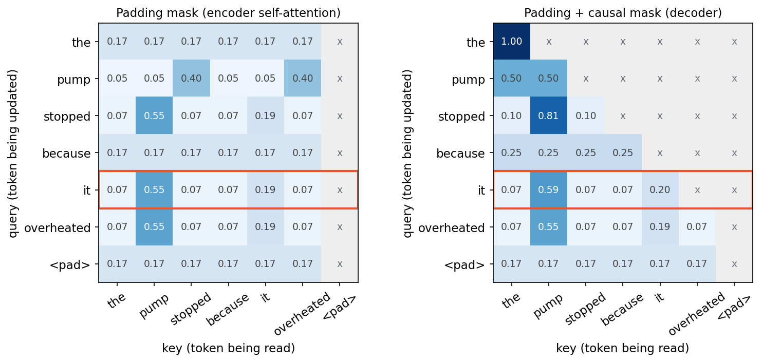
Notice the <pad> row in the figure: a padding query still produces a (meaningless) output, because its keys are not all blocked. This keeps the manual softmax defined for this right-padded example. An all-blocked row makes the ordinary softmax undefined and can produce NaN; kernel behavior for that case should not be assumed. Reject empty real sequences or handle padding-only query rows explicitly, especially when combining left padding with a causal mask. Mask padding keys, and ignore padding outputs in the loss.
6. Multi-head attention
Plain version. Run several smaller attention operations in parallel, each with its own projections, so that different heads can match on different relationships. Then concatenate their outputs and mix them with one more projection.
With heads, head has its own projections :
Here is the scaled dot-product operation of Section 5 with ; the brackets concatenate the outputs (each ) back to width ; and is the output projection. The original Transformer used heads with model width [6]. Because each head is times narrower, multi-head attention costs about as much as one full-width head, and its four projection matrices hold weights (plus biases), the same count as in ML 05.
One head forms one weighted average per query. If a verb needs both its subject and its object, a single softmax must split its weight between them, blurring both. Several heads can each concentrate on one relationship. Do not over-read this: heads are not guaranteed to learn human-readable roles, and some are redundant.
Two later variants change only how keys and values are shared. Multi-query attention uses one key head and one value head for all query heads, which shrinks the memory read at every decoding step [15]. Grouped-query attention shares each key/value head among a group of query heads, an intermediate point between the two [16]. Both matter mainly for fast autoregressive decoding, discussed in NLP 09.
7. Self-attention and cross-attention
Plain version. The same operation connects tokens within one sequence (self-attention) or connects one sequence to another (cross-attention). The only change is where the queries, keys and values come from.
| Mechanism | Queries from | Keys and values from | Typical use in NLP |
|---|---|---|---|
| Bidirectional self-attention | the sequence | the same sequence, all real tokens | encoders such as BERT; the source side of a translator |
| Causal self-attention | the sequence | the same sequence, current and earlier positions | decoder-only language models; the target side of a translator |
| Cross-attention | the decoder | the encoder outputs | encoder–decoder translation and summarization |
For cross-attention, let be decoder states and the encoder outputs (often called the memory):
Here and are the target and source lengths; the score matrix has shape , one row per target position; blocks source padding; and has one output per target position. This is Bahdanau and Luong attention with learned query, key and value projections. No causal mask is needed here, because the source is fully known before decoding begins.
The task’s available information should determine the mask, not a model name. A sentence classifier may use a bidirectional encoder because the complete sentence is available. A streaming continuation must exclude future output tokens. Translation can use the entire source after it arrives, but simultaneous translation, which starts speaking before the source sentence ends, needs a more restrictive source visibility rule.
8. Masks: padding and causal
Plain version. A mask is a table that says which query may read which key. Padding masks hide artificial filler tokens; causal masks hide the future.
For causal self-attention, when and otherwise. Here is the query position and is the candidate key position. With shifted targets, the current input position is an allowed prefix token, so the diagonal remains visible. A fully bidirectional self-attention layer permits every real input position, although padding can still be blocked. For a padding mask, whenever key is a padding position, for every query . Masks combine by blocking a pair if either mask blocks it.
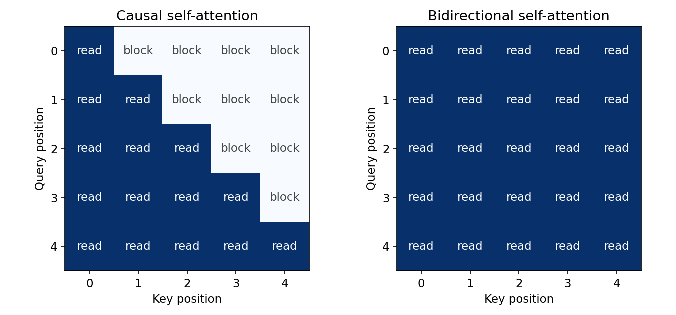
Two different masks are easy to confuse. An attention mask controls what representations may read. A loss mask controls which target positions contribute to the training objective. Padding needs both: padded keys must not contribute context, and padded targets must not contribute loss. They solve different problems and should be tested independently.
A Boolean mask’s meaning also depends on the API. In PyTorch’s scaled_dot_product_attention, True means a pair is allowed [22]. In MultiheadAttention, True in attn_mask means blocked, and True in key_padding_mask marks an ignored key [23]. Name the logical relation first (allowed or blocked) and convert explicitly. Reusing the same Boolean array can silently reverse the information-flow rule. Floating-point masks instead add score biases, such as zero or negative infinity; a floating array of zeros and ones is not the same as a Boolean mask.
The following independent example uses identity projections and uniform scores to make the expected output visible. The first query reads only the first value; the second averages both. The two APIs agree after the Boolean mask is inverted. SDPA also takes a dropout probability directly, so evaluation must explicitly pass dropout_p=0.0 [22].
Code · Python · 22 lines
import torch
from torch import nn
from torch.nn import functional as F

# Two queries and keys, with zero scores: allowed keys receive equal weights.
q = torch.zeros(1, 2, 2)
k = torch.zeros_like(q)
v = torch.tensor([[[10.0, 0.0], [0.0, 20.0]]])
allowed = torch.tril(torch.ones(2, 2, dtype=torch.bool))
blocked = ~allowed
sdpa = F.scaled_dot_product_attention(q[:, None], k[:, None], v[:, None],
                                     attn_mask=allowed, dropout_p=0.0)[:, 0]
mha = nn.MultiheadAttention(2, 1, bias=False, dropout=0.0, batch_first=True).eval()
with torch.no_grad():
    mha.in_proj_weight.copy_(torch.eye(2).repeat(3, 1))
    mha.out_proj.weight.copy_(torch.eye(2))
    module_out, _ = mha(q, k, v, attn_mask=blocked, need_weights=False)
expected = torch.tensor([[[10.0, 0.0], [5.0, 10.0]]])
assert torch.allclose(sdpa, expected)
assert torch.allclose(module_out, expected)
print('mask conventions agree:', torch.allclose(sdpa, module_out))
print('outputs:', sdpa[0].tolist())
Output
mask conventions agree: True
outputs: [[10.0, 0.0], [5.0, 10.0]]
Inspect attention and test its information flow
This standalone matrix example separates learned scores from the visibility rule. All vectors and projections are synthetic, so the weights have no linguistic interpretation.
Code · Python · 26 lines
import numpy as np

rng = np.random.default_rng(0)
T, d = 5, 8                                   # 5 tokens, 8-dimensional embeddings
X = rng.normal(size=(T, d))                   # token embeddings (+ positions)
Wq, Wk, Wv = (rng.normal(size=(d, d)) / np.sqrt(d) for _ in range(3))

def attention(X, causal):
    Q, K, V = X @ Wq, X @ Wk, X @ Wv
    scores = Q @ K.T / np.sqrt(d)             # (T, T) query-key similarities
    if causal:                                # position t may only look at <= t
        scores = np.where(np.tri(T, dtype=bool), scores, -np.inf)
    w = np.exp(scores - scores.max(axis=1, keepdims=True))
    w /= w.sum(axis=1, keepdims=True)         # softmax over keys
    return w @ V, w

out, w = attention(X, causal=True)
print(np.round(w, 2))

# Changing the LAST token must not change any earlier causal output...
X2 = X.copy(); X2[-1] += 5.0
out2, _ = attention(X2, causal=True)
print("causal: earlier outputs unchanged:", np.allclose(out[:-1], out2[:-1]))
# ...but in a bidirectional encoder every position can see it.
b1, _ = attention(X, causal=False); b2, _ = attention(X2, causal=False)
print("bidirectional: earlier outputs unchanged:", np.allclose(b1[:-1], b2[:-1]))
Output:
Code · 7 lines
[[1.   0.   0.   0.   0.  ]
 [0.88 0.12 0.   0.   0.  ]
 [0.42 0.29 0.29 0.   0.  ]
 [0.28 0.24 0.29 0.19 0.  ]
 [0.34 0.06 0.24 0.11 0.26]]
causal: earlier outputs unchanged: True
bidirectional: earlier outputs unchanged: False
The causal weights are lower-triangular: the first token can only read itself, the last can read everything. The numerical checks illustrate the mask’s visibility rule. More generally, row only aggregates value vectors from positions at most . If its queries, keys and values were computed from states that also exclude future information, future inputs cannot affect that output. This condition must hold throughout the network, including any preprocessing that mixes positions. The same mask permits parallel evaluation of all next-token training losses while keeping each prediction restricted to its own prefix.
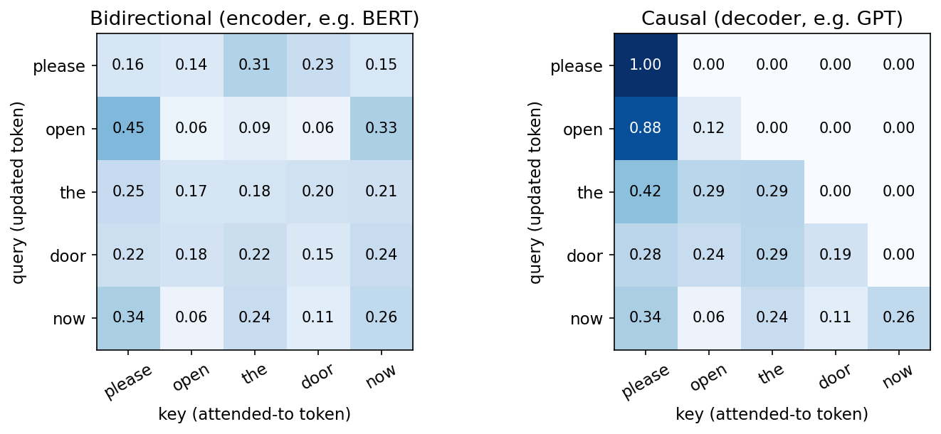
A perturbation test like this one is worth keeping in any real code base. Low training loss cannot reveal a leaking mask, because a model that can see the answer also achieves low loss; only a test that changes a future input and checks earlier outputs targets the visibility contract directly.
9. Position: telling attention where tokens are
Plain version. Attention compares token representations, and position information tells it where those tokens occur. A token’s identity alone does not say whether it is the subject or the final word.
Without position information, self-attention is permutation-equivariant: shuffle the input tokens and the outputs are shuffled the same way, because nothing in the formula refers to order. “Dog bites man” and “man bites dog” would produce the same set of vectors. The encoder-block code in Section 10 checks this property and shows that adding positions breaks it.
The simplest fix adds a position vector to each token embedding before the first layer. For a learned embedding and position table:
Here is the initial representation at position ; is a token embedding table; selects the row for token ; is a position table; selects the position row; and is representation width. A learned position table also imposes a maximum supported position. Giving a sequence beyond that range is not an ordinary longer input; it is an invalid lookup. Record context limits in the serving contract. Extending the table or changing positional behavior is a model change that should be evaluated, rather than assumed to preserve performance on longer documents.
The original Transformer instead used fixed sinusoidal encodings [6]:
Here is the position and indexes a pair of dimensions, each pair rotating at its own frequency. This is the same formula as in ML 05, written there as ; that page proves the two properties that make it useful (a fixed offset acts as a rotation, and dot products depend only on the offset) and plots the pattern. The original paper also multiplies token embeddings by before adding the encoding [6]; the translation model in NLP 08 follows that convention.
Later schemes put position into the attention score itself, so that the model sees relative offsets:
- Relative position representations add learned vectors that depend on the clipped offset to the keys and values [9].
- Rotary position embedding (RoPE) rotates each query and key by an angle proportional to its position, so the score depends on positions only through [10].
- ALiBi adds a fixed, head-specific penalty proportional to the distance to each causal attention score, and was designed so that a model trained on short inputs can be evaluated on longer ones [11].
The choice interacts with the context-length contract. A learned absolute table has a hard maximum; relative methods remove that hard limit but do not guarantee good accuracy beyond the lengths seen in training. Evaluate at the lengths you intend to serve.
10. The Transformer encoder and decoder blocks
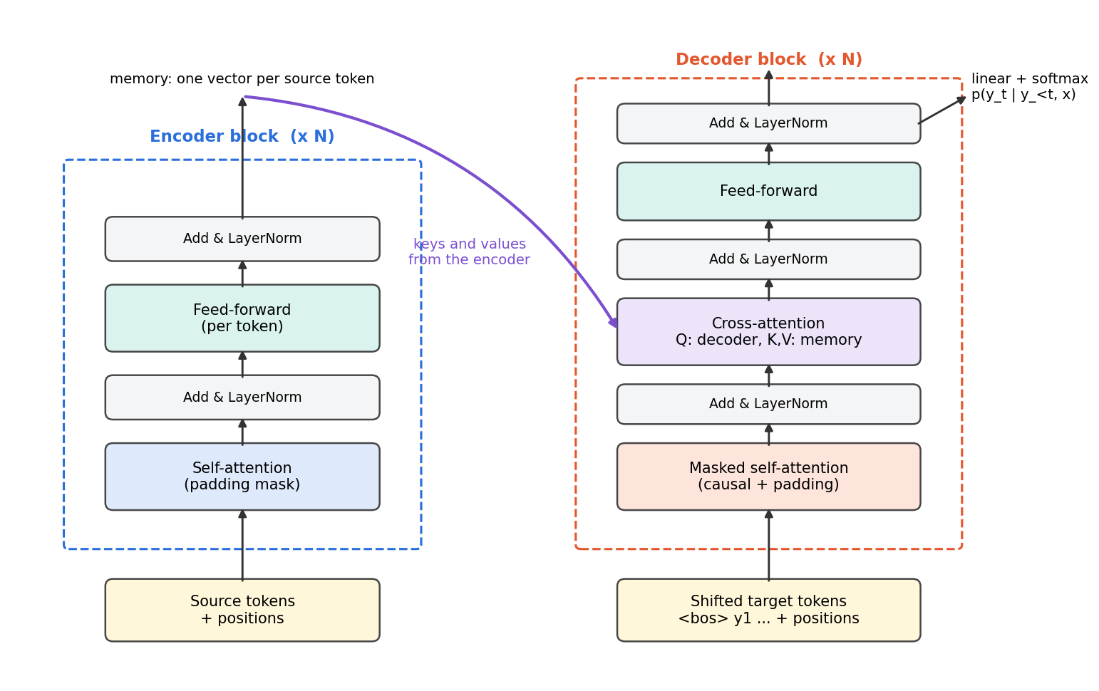
Plain version. A block alternates two jobs. Attention lets tokens exchange information; a small feedforward network then processes each token on its own. Residual connections and normalization keep a deep stack trainable. The decoder adds one more job between them: reading the encoder through cross-attention.
The original encoder block [6] wraps each sublayer in a residual connection followed by layer normalization (post-norm):
Here is the block input; is multi-head self-attention with a padding mask; is layer normalization, which standardizes each token’s features and applies a learned scale and shift [7]; is applied to each position separately with , and a hidden width (2048 for in the original); and is the block output. Many later models move the normalization before each sublayer (pre-norm, ). Xiong et al. analyzed why post-norm needs a learning-rate warm-up while pre-norm can train without one [8]. So “a Transformer” is not fully specified until you say where normalization goes.
The decoder block has three sublayers, each with its own residual connection and normalization:
- Masked self-attention over the target prefix, with a causal mask (and a padding mask for batches).
- Cross-attention, with queries from step 1 and keys and values from the final encoder output, masked only for source padding.
- A position-wise feedforward network.
Stacking encoder blocks and decoder blocks gives the full model ( in the original [6]). Every decoder block reads the same final encoder output. A linear layer and a softmax over the target vocabulary turn the last decoder state into . Dropping the encoder and the cross-attention leaves a decoder-only model, the shape of most current large language models (NLP 09); dropping the decoder leaves an encoder-only model such as BERT (NLP 10).
Code: a tiny Transformer encoder block from scratch
The following code implements multi-head self-attention and a post-norm encoder block directly from the equations, borrows the randomly initialized weights of PyTorch’s nn.TransformerEncoderLayer [21], and checks that both give the same output. It then tests three properties: padding is ignored, the block is permutation-equivariant without positions, and sinusoidal positions break that symmetry. Dropout is off and the reference layer is in evaluation mode so the comparison is exact.
Code · Python · 43 lines
import math
import torch
from torch import nn
from torch.nn import functional as F

torch.manual_seed(0)
B, T, d, h, d_ff = 2, 6, 16, 4, 64
ref = nn.TransformerEncoderLayer(d, h, d_ff, dropout=0.0, activation="relu",
                                 batch_first=True, norm_first=False).eval()

def multi_head_attention(x, key_padding, p):
    q, k, v = (x @ p.in_proj_weight.T + p.in_proj_bias).chunk(3, dim=-1)
    split = lambda t: t.view(B, T, h, d // h).transpose(1, 2)        # (B, h, T, d/h)
    q, k, v = split(q), split(k), split(v)
    scores = q @ k.transpose(-2, -1) / math.sqrt(d // h)               # (B, h, T, T)
    scores = scores.masked_fill(key_padding[:, None, None, :], float("-inf"))
    heads = scores.softmax(dim=-1) @ v                                  # (B, h, T, d/h)
    concat = heads.transpose(1, 2).reshape(B, T, d)                     # heads side by side
    return concat @ p.out_proj.weight.T + p.out_proj.bias

def encoder_block(x, key_padding, layer=ref):
    # Post-norm, as in the original Transformer: x <- LN(x + Sublayer(x))
    a = multi_head_attention(x, key_padding, layer.self_attn)
    x = F.layer_norm(x + a, (d,), layer.norm1.weight, layer.norm1.bias, layer.norm1.eps)
    f = layer.linear2(F.relu(layer.linear1(x)))
    return F.layer_norm(x + f, (d,), layer.norm2.weight, layer.norm2.bias, layer.norm2.eps)

x = torch.randn(B, T, d)
pad = torch.tensor([[False] * 6, [False] * 4 + [True] * 2])     # second sentence: 4 real tokens
with torch.no_grad():
    ours, theirs = encoder_block(x, pad), ref(x, src_key_padding_mask=pad)
    print("matches nn.TransformerEncoderLayer:", torch.allclose(ours[~pad], theirs[~pad], atol=1e-5))
    x2 = x.clone(); x2[1, 4:] = 100.0                             # garbage in padded slots
    print("padding is ignored:", torch.allclose(encoder_block(x2, pad)[~pad], ours[~pad], atol=1e-5))
    perm = torch.tensor([3, 0, 5, 1, 4, 2])
    none = torch.zeros(B, T, dtype=torch.bool)
    y, yp = encoder_block(x, none), encoder_block(x[:, perm], none)
    print("no positions -> permutation-equivariant:", torch.allclose(yp, y[:, perm], atol=1e-5))
    pos = torch.arange(T)[:, None] / 10000 ** (torch.arange(0, d, 2) / d)
    pe = torch.stack([pos.sin(), pos.cos()], dim=-1).flatten(1)     # sin/cos interleaved
    y, yp = encoder_block(x + pe, none), encoder_block(x[:, perm] + pe, none)
    print("with positions -> still equivariant:", torch.allclose(yp, y[:, perm], atol=1e-5))
print("parameters:", sum(p.numel() for p in ref.parameters()))
Output:
Code · 5 lines
matches nn.TransformerEncoderLayer: True
padding is ignored: True
no positions -> permutation-equivariant: True
with positions -> still equivariant: False
parameters: 3280
The comparison uses only real tokens: in evaluation mode PyTorch may take a fused path that does not compute meaningful values at padded positions, and those outputs are ignored anyway. The parameter count checks the formulas: attention has weights and biases, the feedforward network , and the two layer norms . Notice where the parameters live: in this block, as in the original Transformer, the feedforward network holds most of them.
The model has no positional information until we add it, which is exactly what the third and fourth checks show. In a real model, the position vectors are added once, at the input of the first block; every later block inherits order information through the residual stream.
Optional: Transformer (in the Paper guides). Follow the original figure, objective, experimental comparisons and limitations.
11. Cost and long-context variants
Plain version. Every query compares itself with every key, so the work and the score table grow with the square of the sequence length. That is cheap for a sentence and expensive for a book.
For a sequence of length and width , one self-attention layer computes and in about multiply–adds each, plus about for the projections. A recurrent layer costs about but needs sequential steps, whereas all positions of a self-attention layer can be computed in parallel, and any two positions are connected by a path of length one. Vaswani et al. summarize this trade-off in their comparison of layer types [6]. For short sentences ( smaller than ), self-attention is the cheaper of the two; for long documents the term dominates.
Direct attention score storage grows quadratically with sequence length. Specialized implementations can avoid materializing every intermediate matrix, but the modeling question remains which positions need to interact. In deployment, benchmark memory and latency under the actual context lengths rather than extrapolating from a short sentence.
Approaches to long contexts fall into a few families. Tay et al.’s survey organizes them as fixed patterns, learnable patterns, low-rank and kernel methods, memory, recurrence and downsampling [17]. Representative examples:
| Idea | Example | What changes |
|---|---|---|
| Restrict which pairs interact | Longformer: a sliding local window plus a few global tokens [12] | cost grows linearly with for a fixed window; distant tokens communicate through global tokens or several layers |
| Replace the softmax kernel | linear attention with a feature map [13] | scores factorize, giving linear cost and a recurrent view of causal attention; the attention function is different |
| Keep exact attention, move less memory | FlashAttention: tiled, IO-aware computation [14] | same result as standard attention, less memory traffic; quadratic arithmetic remains |
| Share keys and values across heads | multi-query and grouped-query attention [15, 16] | smaller key/value cache during decoding |
| Position schemes that extend | relative, rotary, ALiBi [9–11] | removes a hard positional limit; accuracy at unseen lengths must still be measured |
These are not interchangeable. FlashAttention computes the same function as standard attention; Longformer and linear attention compute different functions and need to be evaluated as different models. State-space and recurrent alternatives that avoid pairwise scores entirely are discussed in ML 04 and ML 05.
Modern view
Plain version. The attention block of 2017 is still recognizable in current models; most changes concern normalization placement, position handling, key/value sharing and efficient kernels, not the core equation.
Surveys. Lin, Wang, Liu and Qiu’s survey of Transformer variants (AI Open, 2022) first describes the original model, then proposes a taxonomy and reviews variants from three perspectives: architectural modification, pretraining, and applications [18]. It is a good map for locating a variant (“is this a change to attention, to position, or to the block?”). Tay, Dehghani, Bahri and Metzler’s Efficient Transformers: A Survey (ACM Computing Surveys, 2022) focuses on the memory and compute of attention and classifies efficient models by mechanism (the families in Section 11) [17]. Its practical message is that efficiency claims depend on sequence length, hardware and implementation, so compare models at the lengths you need.
Attention as explanation. Jain and Wallace reported that attention weights in their models often did not agree with gradient-based importance measures and that very different attention distributions could yield the same prediction [19]. Wiegreffe and Pinter argued that whether attention can serve as an explanation depends on what is meant by explanation, and proposed tests for it [20]. Taken together: an attention map shows where a computation read from, which is useful for debugging masks and alignments, but it is not by itself evidence for why a model made a decision.
State of practice, 2023–2026. Grouped-query attention [16] and IO-aware exact attention kernels [14] address the two costs that dominate serving: key/value memory during decoding and memory traffic during attention. Relative position methods such as RoPE [10] and ALiBi [11] are designed to remove the hard maximum length of a learned position table. Encoder–decoder Transformers remain a natural fit for tasks with a clear source and target, such as translation (NLP 08), while decoder-only models dominate open-ended generation (NLP 09).
Open problems. Reliable use of very long contexts (a longer window permits more input but does not guarantee that all of it is used), length generalization beyond training lengths, the cost of attention over long documents, and faithful interpretation of what attention heads compute.
Key takeaways
- A single context vector forces the whole source through a fixed-size bottleneck; attention lets every output step read every source position.
- Bahdanau attention scores with a small feedforward network; Luong’s dot and general scores reduce attention to matrix products, which leads directly to queries, keys and values.
- Scaled dot-product attention is ; multi-head attention runs narrower copies at about the cost of one.
- Self-attention mixes a sequence with itself; cross-attention lets a decoder read the encoder. The mask, not the weights, decides what each position may read.
- Mask padding keys, mask the future in causal models, keep loss masks separate, and test visibility with a perturbation check.
- Attention ignores order; learned, sinusoidal, relative, rotary or ALiBi positions supply it, each with a different length contract.
- Attention cost grows with ; long-context variants either change the function (sparse, linear) or compute the same function more efficiently (FlashAttention).
Exercises
- Remove the causal mask from the information-flow example in Section 8. Which printed check changes, and why could a language model trained without the mask still show a low training loss?
Hint
The changed final token becomes visible to earlier positions. Low loss can reward access to information that is unavailable during generation.
- In the toy-sentence code, add a second device noun (“valve”) before the pronoun. What happens to the weights of
it? What would a model need, beyond these hand-built features, to choose the right antecedent?
Hint
With identical features, the two devices receive equal scores. Position information, the verb’s meaning and discourse context must enter the query or key to break the tie.
- Design attention and loss masks for a batch of two target sequences of lengths 3 and 5, padded to 5, in a causal decoder. Write the blocked/allowed table for each sequence and the list of target positions that contribute to loss.
Hint
Padding keys must not contribute context, and padding targets must not contribute loss. Decide how a padding query row is handled without creating an all-blocked softmax row.
- For a model with , and , count the weights in one encoder block and one decoder block (ignore biases and layer norms). What fraction of the encoder block is in the feedforward network?
Hint
Self-attention and cross-attention each have weights; the feedforward network has . The decoder has one more attention sublayer than the encoder.
- For sequence lengths , and with , compare (attention scores) with (projections). At which length does the score term start to dominate?
Hint
The two terms are equal when . Below that, the projections cost more than the score computation.
- Explain why Luong’s “general” score is a special case of scaled dot-product attention. What would the query, key and value projections be?
Hint
Absorb into the key projection. The value projection is the identity, and the scale factor is 1.
References
- Masato Hagiwara, Real-World Natural Language Processing: Practical Applications with Deep Learning, Chapter 8, Manning, 2021. Publisher · Chapter 8
- I. Sutskever, O. Vinyals and Q. V. Le, “Sequence to Sequence Learning with Neural Networks,” NeurIPS, 2014. Paper
- K. Cho, B. van Merriënboer, C. Gulcehre, D. Bahdanau, F. Bougares, H. Schwenk and Y. Bengio, “Learning Phrase Representations using RNN Encoder–Decoder for Statistical Machine Translation,” EMNLP, 2014. Paper
- D. Bahdanau, K. Cho and Y. Bengio, “Neural Machine Translation by Jointly Learning to Align and Translate,” ICLR, 2015. Paper
- M.-T. Luong, H. Pham and C. D. Manning, “Effective Approaches to Attention-based Neural Machine Translation,” EMNLP, 2015. Paper
- A. Vaswani et al., “Attention Is All You Need,” NeurIPS, 2017. Paper
- J. L. Ba, J. R. Kiros and G. E. Hinton, “Layer Normalization,” arXiv:1607.06450, 2016. Paper
- R. Xiong et al., “On Layer Normalization in the Transformer Architecture,” ICML, 2020. Paper
- P. Shaw, J. Uszkoreit and A. Vaswani, “Self-Attention with Relative Position Representations,” NAACL, 2018. Paper
- J. Su, M. Ahmed, Y. Lu, S. Pan, W. Bo and Y. Liu, “RoFormer: Enhanced Transformer with Rotary Position Embedding,” Neurocomputing 568, 2024. DOI
- O. Press, N. A. Smith and M. Lewis, “Train Short, Test Long: Attention with Linear Biases Enables Input Length Extrapolation,” ICLR, 2022. Paper
- I. Beltagy, M. E. Peters and A. Cohan, “Longformer: The Long-Document Transformer,” arXiv:2004.05150, 2020. Paper
- A. Katharopoulos, A. Vyas, N. Pappas and F. Fleuret, “Transformers are RNNs: Fast Autoregressive Transformers with Linear Attention,” ICML, PMLR 119, 2020. Paper
- T. Dao, D. Y. Fu, S. Ermon, A. Rudra and C. Ré, “FlashAttention: Fast and Memory-Efficient Exact Attention with IO-Awareness,” NeurIPS, 2022. Paper
- N. Shazeer, “Fast Transformer Decoding: One Write-Head is All You Need,” arXiv:1911.02150, 2019. Paper
- J. Ainslie, J. Lee-Thorp, M. de Jong, Y. Zemlyanskiy, F. Lebrón and S. Sanghai, “GQA: Training Generalized Multi-Query Transformer Models from Multi-Head Checkpoints,” EMNLP, 2023. Paper
- Y. Tay, M. Dehghani, D. Bahri and D. Metzler, “Efficient Transformers: A Survey,” ACM Computing Surveys 55(6), 2022. DOI
- T. Lin, Y. Wang, X. Liu and X. Qiu, “A Survey of Transformers,” AI Open 3, 2022. DOI
- S. Jain and B. C. Wallace, “Attention is not Explanation,” NAACL, 2019. Paper
- S. Wiegreffe and Y. Pinter, “Attention is not not Explanation,” EMNLP-IJCNLP, 2019. Paper
- PyTorch,
TransformerEncoderLayerdocumentation. Documentation - PyTorch,
scaled_dot_product_attentiondocumentation, version 2.15, accessed 2026-11-05. Documentation - PyTorch,
MultiheadAttentiondocumentation, version 2.15, accessed 2026-11-05. Documentation
Check your understanding
This tutorial has 6 exercises. Can you solve them without opening the hints?
Go to the exercises ↑Next NLP 08 · Sequence-to-Sequence Models with Transformers (Machine Translation, Chatbots) · 32 min