NLP 06 · Sequence Labeling with RNNs (POS Tagging, Information Extraction)
Needs: NLP 05 · Recurrent Neural Networks for Language
Navigate: this page and this track: Navigate: this page and this track
On this page
- What you’ll learn1 min
- The big picture2 min
- Words, morphology and grammatical categories1 min
- Local classification versus sequence prediction1 min
- Hidden Markov models for tags1 min
- Maximum-path decoding4 min
- Entity recognition starts with a schema2 min
- Sequence labels and span prediction3 min
- Exact span evaluation1 min
- A complete CPU extraction experiment1 min
- Information extraction beyond entity spans2 min
- Neural taggers: a BiLSTM over the sentence2 min
- BiLSTM-CRF: scoring the whole label sequence2 min
- Character-level features1 min
- Datasets for tagging and extraction2 min
- A complete PyTorch tagging experiment4 min
- Modern view3 min
- Key takeaways1 min
- Exercises2 min
- Paper guides
- References
Natural Language Processing
Explore this chapter 1 interactive experiment
Combine emission scores, transition scores and BIO span constraints to choose a complete tag path.
What you’ll learn
- Represent part-of-speech tagging and entity recognition as sequence labeling, and explain why independent token decisions can disagree with a valid sentence-level analysis.
- Derive hidden Markov sequence scores and maximum-path (Viterbi) decoding, and connect them to the conditional random field.
- Define an entity schema with reproducible offsets, encode mentions with BIO labels, and evaluate exact spans rather than token accuracy.
- Build BiLSTM taggers, add character-level features and a CRF output layer, and train the CRF by its log-likelihood with a masked forward algorithm.
- Place entity tagging inside information extraction (entities, relations, events) and name the standard datasets.
- Run a complete PyTorch experiment that measures span F1, error types and invalid tag transitions on names never seen in training.
The big picture
Many language tasks ask for one label per token. A part-of-speech (POS) tagger marks each word as noun, verb, adjective and so on. An entity recognizer marks which tokens belong to a person, organization or place name, and where each name begins and ends. Both look like classification repeated along a sentence, but they are not independent decisions: the right label for a word depends on its neighbors’ words and on its neighbors’ labels. Treating the whole label sequence as one structured output is the central idea of this chapter.
McRoy’s Chapters 3 and 4 introduce grammatical categories and syntactic processing, and Chapter 8 connects language processing with information extraction [1]. Hagiwara’s Chapter 5 develops sequential labeling, including part-of-speech tagging and named entity recognition [2]. This chapter combines those views. A tagger attaches categories to positions; an extractor turns selected spans into records that an application can inspect. The output contract matters: a customer-support system might need a product name and a complaint event, whereas a historical archive needs people, organizations, dates and attributed statements.
The practical risk is losing distinctions during conversion. “The supplier said the device passed” does not establish that the device passed. A system can identify the correct names and still build a false record by dropping attribution or modality. We therefore evaluate both surface extraction and interpretation, rather than treating well-formed output as evidence of correctness. The structured-prediction mathematics (HMMs, the forward–backward algorithm, Viterbi decoding and CRFs in general form) is developed in PR 06; the recurrent encoders come from NLP 05. Parsing, semantic roles and relation and event extraction in depth follow in NLP 12.
Words, morphology and grammatical categories
Plain version. A word’s category describes how it behaves in a sentence. Its spelling can suggest a category, but context often decides which use is intended.
Morphology concerns structure within words. A plural ending, tense marker or derivational prefix can supply useful evidence, but not every language expresses these properties with the same pieces or word boundaries. Subword tokens learned for efficient modeling also need not correspond to linguistic morphemes. Keep the model’s tokenization separate from the grammatical units used in annotation.
Part of speech describes a grammatical category, such as noun or verb. A noun commonly heads a noun phrase; a verb commonly heads a clause’s predicate. These are distributional descriptions rather than rules that every noun must name a physical object. “Decision” and “arrival” are nouns although they refer to abstract content and events.
The same surface word can have several categories. In the invented pair “the pilots can land” and “the metal can fell,” the word “can” has different roles. The second sentence also demonstrates why a familiar local phrase can be misleading when the remainder of the sentence changes. A tagger must consider the permitted context and its annotation scheme.
Represent a tagged sentence as:
Here is the input word sequence, is the word at position , is sequence length, is the tag sequence, is the tag for word and is the finite tag inventory. The symbols and refer to linguistic word positions, not automatically to model subword positions.
Annotation needs additional rules: contractions, punctuation, multiword expressions and words with several plausible analyses. When a model uses subwords, define how its outputs return to words. Using only the first subword’s representation is one possible convention; pooling all subwords is another. Whatever the choice, gold labels and decoded output must use the same units.
Local classification versus sequence prediction
Plain version. Choosing the best tag for every word separately can miss a better joint interpretation. A sequence model makes the relationship among tags explicit.
A local classifier may predict:
Here is the selected tag at position , ranges over tag inventory , is a model with parameters and is the whole visible input sequence. A local output head can still read contextual input: “independent” describes the output decision rule, not necessarily the encoder.
A structured decoder instead chooses:
Here is the selected complete tag sequence, is the set of permitted analyses for input , and is a score assigned by parameters to an input–analysis pair. The permitted set can enforce an annotation constraint, while the score can reward plausible neighboring labels.
This distinction appears in many NLP tasks. Entity labels must form valid spans; a dependency tree needs one parent per non-root word; a generated structured record must satisfy a schema. A stronger encoder does not automatically guarantee a valid output. The decoder or a separate validator must enforce constraints that the application requires.
Structured decoding also has a tradeoff. An incorrect hard constraint can exclude a legitimate construction. If the grammar says every sentence must contain an overt subject, it will reject many commands and fragments. Document the constraint and its intended input domain rather than treating constrained output as evidence that the constraint was linguistically universal.
Hidden Markov models for tags
Plain version. Imagine that tags form a hidden sequence and each tag generates a word. Neighboring tags and word compatibility then jointly determine the score.
A first-order hidden Markov model (HMM), reviewed by Rabiner [3], uses:
Here is joint probability of words and tags, is the probability of initial tag , is the transition probability from tag to tag , is the probability that tag emits word , and are the word and tag at position , and is sequence length. This example conditions on a fixed length; an explicit end-state factor can be added when modeling termination.
Initial probabilities sum to one. Each transition row sums to one, and each emission distribution sums to one over the observation vocabulary. These normalization conditions make the expression a probability model rather than an arbitrary product of useful scores.
The assumptions are restrictive: the next tag depends only on the previous tag, and an emitted word depends only on the current tag. A real sentence has long dependencies, lexical preferences and discourse context. The value of this model here is that the assumptions and exact decoder are visible. It provides a small laboratory for distinguishing model capacity from search.
With fully tagged training examples, count initial states, transitions and emissions, then normalize with a stated smoothing rule. With words alone, hidden-state estimation is a different problem; a state learned without supervision is not automatically a named grammatical category. The example below uses manually specified probabilities so that training uncertainty does not obscure decoding.
Maximum-path decoding
Plain version. Keep the best partial path ending in each tag. Extending those paths is enough to find the best complete sequence without listing every possibility.
Use log probabilities to turn products into sums:
Here is the log score of the best path covering positions through and ending with tag , is the initial probability, is the emission probability, is the transition probability and is the tag inventory. The indices and identify the previous and current tags. A zero probability contributes .
The recurrence is maximum-path dynamic programming, commonly called Viterbi decoding [3]. For each cell, store the previous tag attaining the maximum. After selecting the best final tag, follow these backpointers in reverse. Keeping only the score loses the actual sequence.
The decoder considers positions and all pairs of adjacent tags, so its time complexity is for tags. The score table uses space if all backpointers are retained. By contrast, enumerating tag sequences considers possibilities. This is a computational saving under a specific factorization, not an approximate search result.
The following standalone example verifies the dynamic-programming answer against exhaustive enumeration. The toy observation “fish fish” has an intentionally ambiguous word. Independent emission preferences select nouns at both positions; the joint model can favor a noun followed by a verb.
Code · Python · 39 lines
import itertools
import numpy as np

tags = ["N", "V"]
vocabulary = ["fish", "swim"]
initial = np.array([0.8, 0.2])
transition = np.array([[0.1, 0.9], [0.8, 0.2]])
emission = np.array([[0.7, 0.3], [0.3, 0.7]])
words = ["fish", "fish"]
observation = [vocabulary.index(word) for word in words]
assert np.allclose(transition.sum(axis=1), 1)
assert np.allclose(emission.sum(axis=1), 1)

scores = np.empty((len(words), len(tags)))
back = np.zeros_like(scores, dtype=int)
scores[0] = np.log(initial) + np.log(emission[:, observation[0]])
for t in range(1, len(words)):
    candidates = scores[t - 1, :, None] + np.log(transition)
    back[t] = candidates.argmax(axis=0)
    scores[t] = candidates.max(axis=0) + np.log(emission[:, observation[t]])
path = [int(scores[-1].argmax())]
for t in range(len(words) - 1, 0, -1):
    path.append(int(back[t, path[-1]]))
path.reverse()

def joint_score(sequence):
    value = np.log(initial[sequence[0]])
    value += np.log(emission[sequence[0], observation[0]])
    for t in range(1, len(words)):
        value += np.log(transition[sequence[t - 1], sequence[t]])
        value += np.log(emission[sequence[t], observation[t]])
    return value

all_paths = list(itertools.product(range(len(tags)), repeat=len(words)))
brute = max(all_paths, key=joint_score)
assert tuple(path) == brute
print("local emission choices:", [tags[emission[:, w].argmax()] for w in observation])
print("best joint path:", [tags[index] for index in path])
print("joint log score:", round(joint_score(path), 3))
Changing transition probabilities changes the chosen sequence even when every word-level preference stays fixed. This does not prove the new choice is correct in real language. It proves that the implemented model and decoder express the intended dependence.
Read the path score as evidence, not just an argmax
The noun–verb path wins in the preceding example because the transition preference outweighs the second word’s emission preference. Its joint probability is the product of four factors: an initial noun, a noun emitting fish, a noun-to-verb transition, and a verb emitting fish. Comparing it with noun–noun cancels the shared first two factors. The remaining comparison is between transition times emission; the decision is therefore intelligible without treating the decoder as a black box.
The following independent calculation enumerates the same four paths and normalizes them into a posterior distribution for the observed words:
Code · Python · 15 lines
import itertools
import numpy as np

initial = np.array([0.8, 0.2])
transition = np.array([[0.1, 0.9], [0.8, 0.2]])
fish = np.array([0.7, 0.3])
paths = list(itertools.product(range(2), repeat=2))
mass = np.array([initial[a] * fish[a] * transition[a, b] * fish[b]
                 for a, b in paths])
posterior = mass / mass.sum()
print('NN / NV / VN / VV joint:', mass.round(4))
print('Posterior:', posterior.round(3))
print('Probability of observed words:', round(mass.sum(), 4))
assert paths[posterior.argmax()] == (0, 1)
assert np.isclose(posterior.sum(), 1)
The joint masses are 0.0392, 0.1512, 0.0336 and 0.0036, and the posterior rounds to 0.172, 0.664, 0.148 and 0.016. The observation probability is 0.2276. These answer different questions. A joint mass includes how likely the words were; a posterior compares label interpretations after those words are fixed. The winning path still leaves probability on alternatives under this constructed model.
For larger sequences, summing predecessor contributions rather than maximizing them computes observation probability. Combining forward and backward contributions gives tag marginals [3]. Selecting the most probable tag at each position minimizes expected per-position mistakes under that posterior; selecting the most probable complete path targets whole-sequence correctness. Those decisions can differ. Independently selected marginal tags can also violate output constraints when the allowed sequence set contains restrictions.
Why can maximum-path decoding discard other prefixes ending in the same tag? Under the first-order factorization, their remaining extensions depend on that final tag and future observations, not on earlier prefix details. A lower-scoring prefix cannot overtake the better prefix after an identical suffix is added. If a new score rewards a relation to a tag several positions earlier, this argument no longer applies to the same state. Either enlarge the state or change the decoder. Exactness belongs to the score factorization, not to the name of the algorithm.
Conditional structured scores connect neural features to decoding
An HMM must model how words are generated. A conditional model can instead score label sequences directly from the observed sentence. A linear-chain conditional random field (CRF) provides this interface [5]:
Here is the observed sentence, is a tag sequence, is its length, indexes positions, is a position–tag score computed with parameters , and contains adjacent-tag scores. The normalizer sums over every permitted sequence . Unlike HMM emissions, the position scores need not sum to one over words. A contextual encoder can compute each score using the entire sentence while the output dependence remains a chain.
Training an annotated sequence minimizes its negative log probability: the correct score is rewarded relative to the scores of all permitted competitors. Computing the normalizer uses a sum recurrence; finding the best sequence uses a max recurrence. This explains why a neural encoder and structured decoder fit together. Rich input evidence does not require discarding a tractable output factorization. Conversely, a chain transition table cannot express every syntactic dependency; sentence-level input features and output constraints solve different parts of the problem.
PR 06 develops the general theory behind these two models: the forward and forward–backward algorithms, Baum–Welch training of HMMs from unlabeled sequences, and the CRF gradient as observed minus expected feature counts. The neural tagger sections below reuse exactly this CRF, with the position scores computed by a recurrent encoder.
Entity recognition starts with a schema
Plain version. An entity recognizer locates mentions and assigns types. It does not automatically identify the unique real-world object behind each mention.
Represent an entity mention as:
Here is a mention record; is the document identifier; is its inclusive starting character offset; is its exclusive ending offset; and is its category. The surface text is the original document slice from to . These are Python string offsets in our example; another interface may use bytes or another indexing convention. Declare the convention because Unicode characters and encoded bytes do not have identical boundaries.
An annotation guideline must decide whether titles belong to a person’s span, whether an organization suffix is included, and how to handle ambiguous uses. “Taipei” can name a place or stand for a government in context. A location-only schema and a context-sensitive organization schema can legitimately produce different annotations. Evaluation becomes meaningful only after the schema and guidelines are frozen.
Named entity recognition, or NER, commonly distinguishes people, organizations and locations; the CoNLL-2003 shared-task paper describes one established benchmark setting [6]. We mention that resource to identify the evaluation tradition, not to imply that its categories fit every application. Product identifiers, legal provisions or equipment parts may be more useful in another domain.
Entity linking is a separate decision: map a mention to a record in a knowledge base, or choose that no suitable record exists. Two mentions with the same spelling can refer to different organizations; two different spellings can refer to the same one. A recognizer that marks “Orion” as an organization has not solved this identity problem. Linking requires a candidate inventory, context and an explicit unknown-entity policy.
Keep the original text and offsets even when you store a normalized name. Lowercasing, accent removal and whitespace collapse can change strings and boundaries. One reliable design extracts from the original text and stores normalization as an additional field. If preprocessing is necessary, retain an alignment map so the predicted span can be projected back without guessing.
Sequence labels and span prediction
Plain version. Entity mentions can be expressed as labels on tokens or as explicit spans. The representation determines which overlaps the model can describe.
In a BIO scheme, a token label begins with B for the beginning of a mention, I for its continuation or O for outside. An example is “Mina works at Orion Labs,” with person labels on Mina and organization labels on Orion and Labs. Hagiwara’s sequence-labeling chapter and the NER survey give context for token-level extraction models [2], [7]. The scheme descends from the inside–outside chunk tags of Ramshaw and Marcus [10].
For an independent token classifier:
Here is the input token sequence; is the label sequence; is the number of tokens; indexes positions; and denotes learned parameters. Each prediction may use a contextual representation of the whole permitted input, although the output labels are independent under this factorization. Input context and output dependence are different ideas.
Independent decisions can produce invalid transitions, such as an I-PER label after O. A deterministic repair rule is possible, but its behavior becomes part of the evaluation contract. Alternatively, a structured decoder searches only valid paths while scoring the whole sequence. The dynamic-programming idea from the maximum-path decoding section applies when the score decomposes locally. More powerful encoders do not remove the need to define valid outputs.
A flat token-label sequence cannot represent arbitrary nested mentions. “Orion Labs Research Division” could contain an organization mention and a nested division mention under a particular schema. A span model instead scores candidate boundaries and types:
Here is a learned score; and are candidate span boundaries; is the candidate category; and is the input. The score need not be a calibrated probability. A selection policy decides which candidates to keep, whether overlap is allowed and how conflicts are resolved.
The candidate count grows with sentence length, so practical designs may bound maximum span length or prune candidates. Every such restriction changes which mentions can be recovered. If very long names matter, measure their recall separately. A fast system can otherwise achieve a reasonable average score while never representing the outputs needed by a small but consequential group of users.
Boundary modeling changes which errors are possible
A token-labeling model and a span model can use the same contextual encoder yet search different output spaces. Flat BIO labels choose a single membership at each token. Explicit spans choose boundary pairs and types, so nested intervals can coexist when the selection policy permits them. The difference is representational: an encoder cannot recover a nested output that its decoder has no way to express [7].
For tokens, the number of nonempty contiguous intervals is . Here is sentence length; the count sums the possible endings for each starting position. With maximum length , the count becomes , where is the permitted span length. A type scorer may need a score for each of those intervals and each category. Bounding length saves work but removes longer mentions from the candidate space before classification begins.
Boundary quality and semantic typing need separate diagnosis. A span covering Orion may be a strong organization candidate while the gold mention is Orion Labs. Raising its category confidence does not fix the missing boundary. A model may instead propose both spans; then deduplication and overlap rules determine the final output. Treat selection as part of the model behavior, not as formatting applied after evaluation.
Relations add another search problem. Candidate entity pairs multiply as more mentions survive. Restricting pairs by type or distance can reduce computation, but a document-level relation may cross several sentences. A joint extractor can use relation evidence to influence mention decisions, whereas a pipeline commits to mentions first. Compare the pipeline on predicted mentions and on gold mentions: the gap reveals how much relation recovery is lost before relation scoring starts.
Exact span evaluation
Plain version. Correctly labeling common background tokens can hide missed entities. Evaluate complete mentions, including their boundaries and types.
For sets of predicted records and gold records :
Here and contain document identifier, start offset, end offset and category tuples; denotes set size; and contains exact matches. Precision measures the share of predictions that match; recall measures the share of annotations recovered; and combines them. Our code reports zero when a displayed denominator is zero; another evaluation convention should be documented explicitly.
Exact matching is strict. Predicting “Orion” when the annotation says “Orion Labs” creates both a false positive and a false negative. That is appropriate when downstream code depends on a complete name. For another application, partial overlap may deserve a secondary diagnostic. Report its matching rule separately; do not rename a forgiving overlap score as the established exact-match measure [6].
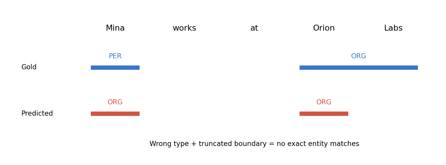
A single aggregate score still hides the mechanism. Break errors into missed mention, spurious mention, boundary mismatch, category mismatch and linking mismatch. Also report performance by category and document source. When a category is rare, retain its example count so the reader can assess uncertainty. A large weighted average can otherwise bury a category with nearly no successful predictions.
A complete CPU extraction experiment
Plain version. A small deterministic extractor makes the contract easy to inspect. It is a teaching baseline with visible blind spots, not a general language-understanding system.
The following standalone example recognizes an invented name inventory, extracts one tightly constrained active repair construction and evaluates exact entity records. It downloads nothing. The inventory is fixed before evaluation, and the gold records are written explicitly. A lexicon is an allowed input here; if a real evaluation forbids external name inventories, the same code would violate that contract.
Code · Python · 46 lines
import re

documents = {
    "a": "Mina repaired Sensor A in Taipei.",
    "b": "Orion Labs said Sensor B might fail.",
    "c": "Leo did not repair Sensor B.",
    "d": "The sensor was repaired by Mina.",
}
inventory = {
    "Mina": "PER", "Leo": "PER", "Orion Labs": "ORG",
    "Sensor A": "DEVICE", "Sensor B": "DEVICE", "Taipei": "LOC",
}
gold = {
    ("a", 0, 4, "PER"), ("a", 14, 22, "DEVICE"), ("a", 26, 32, "LOC"),
    ("b", 0, 10, "ORG"), ("b", 16, 24, "DEVICE"),
    ("c", 0, 3, "PER"), ("c", 19, 27, "DEVICE"), ("d", 27, 31, "PER"),
}
predicted = set()
for doc_id, text in documents.items():
    for name, category in inventory.items():
        pattern = r"(?<!\w)" + re.escape(name) + r"(?!\w)"
        for match in re.finditer(pattern, text):
            predicted.add((doc_id, match.start(), match.end(), category))
tp = len(predicted & gold)
precision = tp / len(predicted) if predicted else 0.0
recall = tp / len(gold) if gold else 0.0
f1 = 2 * tp / (len(predicted) + len(gold)) if predicted or gold else 0.0
assert predicted == gold
print("entity precision/recall/F1:", precision, recall, f1)

repair = re.compile(r"^(Mina|Leo) repaired (Sensor [AB])(?=[ .])")
events = []
for doc_id, text in documents.items():
    match = repair.search(text)
    if match:
        events.append({
            "document": doc_id, "predicate": "repair",
            "actor": match.group(1), "object": match.group(2),
            "polarity": "positive", "modality": "asserted",
            "evidence": [match.start(), match.end()],
        })
assert len(events) == 1 and events[0]["document"] == "a"
for event in events:
    start, end = event["evidence"]
    print(event, "source:", documents[event["document"]][start:end])
print("unsupported repair constructions:", ["c", "d"])
The exact entity score is 1.0 on these hand-built documents, because all mention spellings are in the inventory. That result does not establish generalization. The event rule returns only document a. It excludes the explicit negation in c but also misses the valid passive construction in d. These are different reasons for returning no event, and a production interface should distinguish rejected negative claims from unsupported syntax.
Document b contains recognized entities but no asserted repair event. It also contains an attributed, possible failure. This example illustrates why entity recognition and event extraction need separate evaluation. A system can obtain every name correctly while omitting the task’s most relevant event. Expanding the event grammar requires additional positive and negative fixtures before accepting the new behavior.
The evidence interval covers only the matched clause, not the trailing location. That is adequate for the narrow repair record, which has no location field. If the record later includes location, expand the evidence contract and its tests. Treat schema changes as changes to the task, rather than adding a field that is populated opportunistically from unrelated nearby words.
Information extraction beyond entity spans
Plain version. Entity recognition finds the names. Information extraction (IE) goes on to connect them: which person works for which organization, which device failed where and when. Each step adds a new kind of record and a new way to be wrong.
A useful map has three layers, each building on the previous one.
| Layer | Output record | Example from the running domain | Typical method family |
|---|---|---|---|
| Entities | Typed span | Orion Labs is an ORG at characters 0–10 | Sequence labeling (this chapter) or span scoring |
| Relations | Typed, directed pair of mentions with evidence | employer(Mina, Orion Labs) | Classify candidate mention pairs |
| Events | Trigger plus role-labeled arguments, polarity and modality | repair with repairer Mina, object Sensor A, place Taipei | Trigger detection, then argument labeling |
Sequence labeling contributes directly to all three. Entity mentions are BIO spans. Event triggers can be tagged the same way as entities. Even some relation and argument decisions are posed as labeling, by tagging the tokens of each argument relative to a given trigger. The rule-based extractor above already shows the dependency between layers: its single event record is correct only because both entity spans were found and the construction was supported.
Standard resources reflect the layers. The ACE 2005 multilingual training corpus annotates entities, relations and events for English, Chinese and Arabic, with event annotation limited to English and Chinese [19]. TACRED is a crowdsourced sentence-level relation extraction dataset targeted at the relation types of the TAC Knowledge Base Population evaluation [20]. DocRED moves relation extraction to whole documents built from Wikipedia and Wikidata, where many relations can only be inferred by reading several sentences [21]. The record design questions raised earlier in this chapter (evidence spans, attribution, negation, unknown values) apply at every layer. Relation and event extraction, semantic roles and their evaluation are developed in NLP 12.
Neural taggers: a BiLSTM over the sentence
Plain version. Replace hand-written emission probabilities with a neural network that reads the whole sentence in both directions and produces a score for every tag at every position. The simplest version picks the highest-scoring tag at each position independently.
Collobert and colleagues showed that a single neural architecture, trained from data with little feature engineering, could tag parts of speech, chunks, named entities and semantic roles [12]. With recurrent encoders the standard design is the bidirectional LSTM (BiLSTM) tagger [13], [14], [15]:
Here is the input vector for token (a word embedding, optionally concatenated with character features below); has read and has read ; is concatenation; and map the two states to tag scores; and collects those scores, for tag . These scores play the role of in the CRF formula above: they can depend on the whole sentence. Bidirectionality is appropriate here, unlike in the left-to-right language model of NLP 05, because the whole sentence is given before any tag is chosen [23].
The softmax tagger treats the tags as conditionally independent given these scores:
Here indexes sentences in a mini-batch, is the padding mask (one for a real token), counts real tokens, is the gold tag and ranges over tags. This is exactly the independent token classifier of the sequence-labeling section, with a BiLSTM computing the context. It is fast and often strong. Its weakness is also the one identified there: nothing stops it from emitting O I-ORG, or B-PER I-ORG, because each position’s decision ignores its neighbors’ decisions.
Three practical details matter as much as the architecture.
- Masks. Sentences in a batch are padded to a common length. The mask removes padding from the loss; packing (
pack_padded_sequence) or masking keeps padding out of the backward LSTM, which would otherwise start reading from padding symbols. - Unknown words. A word-embedding table only covers training words. Map the rest to an unknown id, and train that id: randomly replacing a fraction of training words with it (word dropout) teaches the tagger to rely on context when the word itself is unfamiliar.
- Subword encoders. When the encoder uses subwords, define how word labels map to pieces (label the first piece and ignore the others, or another explicit rule) and map predictions back to words before evaluation, as discussed in the first section.
BiLSTM-CRF: scoring the whole label sequence
Plain version. Keep the BiLSTM’s per-token scores, add a learned score for every pair of adjacent tags, and choose the label sequence with the best total. Training raises the score of the gold sequence relative to all other sequences, which the forward algorithm sums efficiently.
Huang, Xu and Yu proposed putting a linear-chain CRF layer on top of a BiLSTM for POS tagging, chunking and NER [13]. Lample and colleagues [14] and Ma and Hovy [15] combined the same output layer with character-level word representations and reported strong NER results without hand-engineered features. Using the CRF notation from the maximum-path decoding section, with start and end scores added:
Here are the BiLSTM scores; is the learned score for tag followed by tag ; and score starting and ending with tag ; and sums over every tag sequence of length . The training loss is the negative log-likelihood averaged over sentences.
The sum over sequences is computed by the forward algorithm in log space:
Here is the log of the summed exponentiated scores of all partial sequences that cover positions to and end in tag . Replacing each log-sum-exp by a maximum, and storing the maximizing , gives exactly the Viterbi recursion of the HMM section with replaced by and by . Both cost . In a padded batch, a position with mask zero copies forward unchanged, so each sentence’s normalizer stops at its own length.
What the gradient does. Differentiating the loss with respect to a transition score gives
where counts how often tag is followed by tag in and the expectation is under the model. Gradient descent therefore raises transitions that the gold sequence uses more often than the model currently expects and lowers the others; the expectations come from forward–backward marginals, as PR 06 shows. Automatic differentiation of the forward algorithm computes this without writing the backward pass by hand.
Hard constraints. A BIO scheme forbids some transitions outright: I-x may only follow B-x or I-x, and no sentence may start with I-x. A learned usually discovers this from data, but with little data it may not. Setting the forbidden entries of and to (in practice a large negative number) makes invalid sequences impossible under both training and decoding, at no cost to valid ones. This is the output-constraint idea from the local-versus-sequence section made concrete.
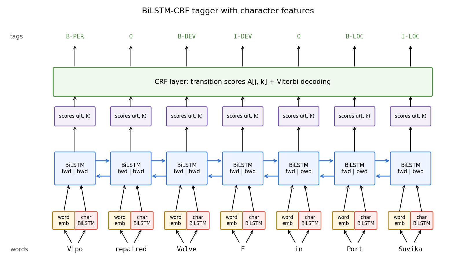
Optional: BiLSTM-CRF (in the Paper guides). Follow the original figure, objective, experimental comparisons and limitations.
Character-level features
Plain version. A word-embedding table knows nothing about a word it never saw. The letters of the word often do: capitalization, suffixes such as “-ville” or “-corp,” digits and hyphens are strong clues to the tag even for a brand-new name.
Before neural taggers, these clues were hand-written features (is capitalized, ends in “-ing,” contains a digit). Neural taggers learn them from characters. Lample and colleagues run a small bidirectional LSTM over each word’s characters and concatenate its final forward and backward states to the word embedding [14]; Ma and Hovy use a convolution over character embeddings followed by max pooling [15]. Either way the input becomes
where is the word embedding, the character summary, the number of characters in , the forward character-LSTM state after the last character and the backward state after reading back to the first. The word-level BiLSTM then reads . Akbik, Blythe and Vollgraf took this idea further: they trained a character-level language model, as in NLP 05, and used its internal states around each word as contextual embeddings for sequence labeling [16].
Character features help with exactly the inputs that word embeddings handle worst: unseen names, rare inflections and misspellings. They do not resolve ambiguity that the spelling does not encode. A name with no telling suffix can be a person or a company, and only context or world knowledge decides. Character inputs also need their own unknown-symbol policy for characters missing from training.
Datasets for tagging and extraction
Plain version. Benchmarks fix a tag inventory, an annotation guideline, a tokenization and a split. Comparing numbers across them is only meaningful when all four match.
| Resource | Task | What it provides |
|---|---|---|
| Penn Treebank [11] | English POS tagging and parsing | A large annotated corpus of English with part-of-speech tags and syntactic bracketing; its tag set is widely used for English |
| Universal Dependencies [4] | Cross-lingual POS, morphology and dependencies | A shared annotation framework applied to treebanks in many languages |
| CoNLL-2003 [6] | Named entity recognition | English and German data with four types (person, organization, location, miscellaneous) and exact-match evaluation |
| OntoNotes [17] | Named entities with 18 types, plus syntax, semantic roles and coreference | Multi-genre, multilingual annotation with stratified training, development and test partitions whose test sets match the CoNLL-2012 shared task |
| WNUT 2017 [18] | Novel and emerging entities in noisy user-generated text | A test of recall on rare and previously unseen surface forms |
| ACE 2005 [19] | Entities, relations and events | Multilingual annotation (English, Chinese, Arabic) used for relation and event extraction |
| TACRED [20] | Sentence-level relation extraction | Crowdsourced relation labels for TAC KBP relation types |
| DocRED [21] | Document-level relation extraction | Entities and relations annotated over Wikipedia documents, requiring multi-sentence reasoning |
Tag encodings differ too. The CoNLL-2003 files use an IOB variant, descended from Ramshaw and Marcus’s chunk tags, in which B- appears only when an entity directly follows another entity of the same type [6], [10]; convert such files to the BIO form used in this chapter before training, or a BIO span extractor will misread them. Licenses differ: some of these resources are freely downloadable, while others are distributed by the Linguistic Data Consortium under license. Check the terms before building on one. For a new domain, the most valuable dataset is usually a small, carefully adjudicated set annotated with your own frozen guideline, used alongside a public benchmark to compare methods.
A complete PyTorch tagging experiment
Plain version. We train three taggers on the same small synthetic corpus and evaluate them on sentences whose names never appear in training: a word-only BiLSTM, the same tagger with character features, and the character tagger with a constrained CRF output layer. The evaluation counts exact spans, error types and invalid tag transitions.
The corpus is invented. Person, organization and location names are generated from random syllables, so test names are new spellings. Organizations either end in tek or corp or are followed by the word Labs; locations either end in ville or follow Port. Several templates allow either a person or an organization in the same slot, so context alone cannot always decide the type. There are 100 training sentences and 200 test sentences. Everything else is implemented from scratch: span extraction from BIO tags, exact span precision, recall and F1, an error breakdown, padding masks, word dropout, the character BiLSTM, and a CRF with a masked forward algorithm, Viterbi decoding and BIO constraints, checked against brute-force enumeration. Each model is trained with three seeds; the script runs on a CPU in well under a minute.
Code · Python · 253 lines
import random
import torch
from torch import nn

# ---- 1. A synthetic tagged corpus: invented names, fixed templates ----
SYL = ["ka", "mi", "to", "re", "na", "lo", "su", "vi", "da", "po", "ri", "ze"]

def coin(rng, kind):
    stem = "".join(rng.choice(SYL) for _ in range(rng.choice((2, 3)))).capitalize()
    if kind == "PER":
        return stem
    if kind == "ORG":
        return rng.choice([stem + rng.choice(["tek", "corp"]), stem + " Labs"])
    return rng.choice(["Port " + stem, stem + "ville"])           # LOC

rng = random.Random(0)
TRAIN_NAMES = {k: sorted({coin(rng, k) for _ in range(40)}) for k in ("PER", "ORG", "LOC")}
seen = {n for v in TRAIN_NAMES.values() for n in v}
TEST_NAMES = {k: rng.sample(sorted({coin(rng, k) for _ in range(60)} - seen), 15)
              for k in ("PER", "ORG", "LOC")}                       # unseen spellings
TRAIN_NAMES["DEV"] = ["Pump A", "Pump B", "Sensor C", "Sensor D", "Valve E", "Valve F"]
TEST_NAMES["DEV"] = ["Pump G", "Sensor H", "Valve J", "Pump K"]
TEMPLATES = [
    "{PER} repaired {DEV} in {LOC} .",
    "{ORG} repaired {DEV} in {LOC} .",
    "{PER} reported a fault in {DEV} .",
    "{ORG} reported a fault in {DEV} .",
    "the sensor near {LOC} was checked by {PER} .",
    "the sensor near {LOC} was checked by {ORG} .",
    "{PER} and {PER} visited {LOC} .",
    "{ORG} shipped {DEV} to {LOC} yesterday .",
    "after the test , {PER} said {DEV} might fail .",
    "a pump in {LOC} failed and {ORG} replaced it .",
]

def make(names, n):
    data = []
    for _ in range(n):
        words, tags = [], []
        for piece in rng.choice(TEMPLATES).split():
            if piece.startswith("{"):
                kind = piece[1:-1]
                toks = rng.choice(names[kind]).split()
                words += toks
                tags += ["B-" + kind] + ["I-" + kind] * (len(toks) - 1)
            else:
                words.append(piece)
                tags.append("O")
        data.append((words, tags))
    return data

train_data, test_data = make(TRAIN_NAMES, 100), make(TEST_NAMES, 200)
TAGS = ["O"] + [f"{p}-{k}" for k in ("PER", "ORG", "LOC", "DEV") for p in "BI"]
t2i = {t: i for i, t in enumerate(TAGS)}
w2i = {w: i + 2 for i, w in enumerate(sorted({w for s, _ in train_data for w in s}))}
c2i = {c: i + 2 for i, c in enumerate(sorted({c for w in w2i for c in w}))}
PAD, UNK = 0, 1
print(train_data[0])

# ---- 2. Spans and exact span F1, from scratch ----
def spans(tags):
    out, start, kind = set(), None, None
    for i, t in enumerate(tags + ["O"]):
        if start is not None and not (t.startswith("I-") and t[2:] == kind):
            out.add((start, i, kind))
            start = None
        if t.startswith("B-") or (t.startswith("I-") and start is None):
            start, kind = i, t[2:]                  # an orphan I- still opens a span
    return out

def span_prf(gold_seqs, pred_seqs):
    tp = n_pred = n_gold = 0
    for g, p in zip(gold_seqs, pred_seqs):
        G, P = spans(g), spans(p)
        tp, n_pred, n_gold = tp + len(G & P), n_pred + len(P), n_gold + len(G)
    prec = tp / n_pred if n_pred else 0.0
    rec = tp / n_gold if n_gold else 0.0
    f1 = 2 * tp / (n_pred + n_gold) if n_pred + n_gold else 0.0
    return prec, rec, f1

def error_types(gold_seqs, pred_seqs):
    counts = {"type": 0, "boundary": 0, "missed": 0, "spurious": 0}
    for g, p in zip(gold_seqs, pred_seqs):
        G, P = spans(g), spans(p)
        overlap = lambda a, b: a[0] < b[1] and b[0] < a[1]
        for s in G - P:
            hits = [q for q in P if overlap(s, q)]
            if any(q[:2] == s[:2] for q in hits):
                counts["type"] += 1             # right boundaries, wrong category
            elif hits:
                counts["boundary"] += 1         # overlaps, wrong boundaries
            else:
                counts["missed"] += 1
        counts["spurious"] += sum(not any(overlap(q, s) for s in G) for q in P - G)
    return counts

def invalid(tags):                                  # I-x not preceded by B-x or I-x
    return sum(t.startswith("I-") and (i == 0 or tags[i - 1][2:] != t[2:])
               for i, t in enumerate(tags))

assert spans(["B-ORG", "I-ORG", "O", "B-PER"]) == {(0, 2, "ORG"), (3, 4, "PER")}
assert invalid(["O", "I-LOC", "B-DEV", "I-DEV"]) == 1
print("train/test sentences:", len(train_data), len(test_data),
      " gold test spans:", sum(len(spans(t)) for _, t in test_data))

# ---- 3. Padding, masks and word dropout ----
def batch(data, unk_rate=0.0, r=None):
    L = max(len(s) for s, _ in data)
    W = max(len(w) for s, _ in data for w in s)
    x = torch.full((len(data), L), PAD)
    c = torch.full((len(data), L, W), PAD)
    y = torch.zeros(len(data), L, dtype=torch.long)
    for b, (s, t) in enumerate(data):
        for i, w in enumerate(s):
            drop = r is not None and r.random() < unk_rate
            x[b, i] = UNK if drop else w2i.get(w, UNK)      # train the unknown id too
            y[b, i] = t2i[t[i]]
            for j, ch in enumerate(w):
                c[b, i, j] = c2i.get(ch, UNK)
    return x, c, y, x != PAD

# ---- 4. BiLSTM encoder with optional character BiLSTM features ----
class Encoder(nn.Module):
    def __init__(self, use_chars, wdim=32, cdim=16, hidden=48):
        super().__init__()
        self.use_chars = use_chars
        self.wemb = nn.Embedding(len(w2i) + 2, wdim, padding_idx=PAD)
        self.cemb = nn.Embedding(len(c2i) + 2, cdim, padding_idx=PAD)
        self.clstm = nn.LSTM(cdim, cdim, batch_first=True, bidirectional=True)
        self.lstm = nn.LSTM(wdim + (2 * cdim if use_chars else 0), hidden,
                            batch_first=True, bidirectional=True)
        self.emit = nn.Linear(2 * hidden, len(TAGS))

    def forward(self, x, c):
        feats = [self.wemb(x)]
        if self.use_chars:
            B, L, W = c.shape
            lengths = (c != PAD).sum(-1).clamp(min=1).view(-1)
            packed = nn.utils.rnn.pack_padded_sequence(
                self.cemb(c.view(B * L, W)), lengths, batch_first=True,
                enforce_sorted=False)
            _, (h, _) = self.clstm(packed)          # last forward + first backward state
            feats.append(torch.cat([h[0], h[1]], -1).view(B, L, -1))
        h, _ = self.lstm(torch.cat(feats, -1))
        return self.emit(h)                         # emission scores u[b, t, k]

# ---- 5. Linear-chain CRF with BIO constraints and a padding mask ----
class CRF(nn.Module):
    def __init__(self, K):
        super().__init__()
        self.A = nn.Parameter(torch.zeros(K, K))    # A[j, k]: score of tag j -> tag k
        self.start = nn.Parameter(torch.zeros(K))
        self.end = nn.Parameter(torch.zeros(K))
        ban = torch.zeros(K, K)                     # I-x only after B-x or I-x
        for k, tag in enumerate(TAGS):
            if tag.startswith("I-"):
                ban[:, k] = -1e4
                ban[t2i["B-" + tag[2:]], k] = ban[k, k] = 0.0
        self.register_buffer("ban", ban)
        self.register_buffer("ban_start", torch.tensor(
            [-1e4 if t.startswith("I-") else 0.0 for t in TAGS]))

    def trans(self):
        return self.A + self.ban

    def score(self, u, y, mask):                    # S(x, y) for the gold path
        s = (self.start + self.ban_start)[y[:, 0]] + u[:, 0].gather(1, y[:, :1]).squeeze(1)
        for t in range(1, u.size(1)):
            step = self.trans()[y[:, t - 1], y[:, t]] + u[:, t].gather(1, y[:, t:t + 1]).squeeze(1)
            s = s + step * mask[:, t]
        last = y.gather(1, (mask.sum(1) - 1).unsqueeze(1)).squeeze(1)
        return s + self.end[last]

    def log_partition(self, u, mask):               # forward algorithm in log space
        alpha = self.start + self.ban_start + u[:, 0]
        for t in range(1, u.size(1)):
            nxt = torch.logsumexp(alpha.unsqueeze(2) + self.trans() + u[:, t].unsqueeze(1), dim=1)
            alpha = torch.where(mask[:, t:t + 1], nxt, alpha)   # padding: carry forward
        return torch.logsumexp(alpha + self.end, dim=1)

    def nll(self, u, y, mask):
        return (self.log_partition(u, mask) - self.score(u, y, mask)).mean()

    def viterbi(self, u, mask):                     # same recursion with max + backpointers
        delta, back = self.start + self.ban_start + u[:, 0], []
        for t in range(1, u.size(1)):
            best, arg = (delta.unsqueeze(2) + self.trans()).max(1)
            back.append(arg)
            delta = torch.where(mask[:, t:t + 1], best + u[:, t], delta)
        delta = delta + self.end
        paths = []
        for b in range(u.size(0)):
            k = int(delta[b].argmax())
            path = [k]
            for t in range(int(mask[b].sum()) - 1, 0, -1):
                k = int(back[t - 1][b, k])
                path.append(k)
            paths.append(path[::-1])
        return paths

# Check the masked forward algorithm and Viterbi against brute-force enumeration
import itertools
torch.manual_seed(0)
check = CRF(len(TAGS))
with torch.no_grad():
    check.A.normal_()
u = torch.randn(1, 3, len(TAGS))
m = torch.ones(1, 3, dtype=torch.bool)
paths = [torch.tensor([p]) for p in itertools.product(range(len(TAGS)), repeat=3)]
scores = torch.stack([check.score(u, p, m)[0] for p in paths])
assert torch.allclose(check.log_partition(u, m)[0], torch.logsumexp(scores, 0), atol=1e-4)
assert paths[int(scores.argmax())][0].tolist() == check.viterbi(u, m)[0]

# ---- 6. Train three taggers and evaluate exact spans on unseen names ----
def run(use_chars, use_crf, seed, epochs=15):
    torch.manual_seed(seed)
    r = random.Random(seed)
    enc, crf = Encoder(use_chars), CRF(len(TAGS))
    params = list(enc.parameters()) + (list(crf.parameters()) if use_crf else [])
    opt = torch.optim.Adam(params, lr=5e-3)
    order = list(range(len(train_data)))
    for _ in range(epochs):
        r.shuffle(order)
        for i in range(0, len(order), 32):
            x, c, y, mask = batch([train_data[j] for j in order[i:i + 32]], 0.25, r)
            u = enc(x, c)
            loss = (crf.nll(u, y, mask) if use_crf      # sequence-level loss
                    else nn.functional.cross_entropy(u[mask], y[mask]))  # per token
            opt.zero_grad()
            loss.backward()
            nn.utils.clip_grad_norm_(params, 5.0)
            opt.step()
    enc.eval()
    with torch.no_grad():
        x, c, y, mask = batch(test_data)
        u = enc(x, c)
        pred = (crf.viterbi(u, mask) if use_crf else
                [u[b, :int(mask[b].sum())].argmax(-1).tolist() for b in range(len(u))])
    pred = [[TAGS[k] for k in p] for p in pred]
    gold = [t for _, t in test_data]
    return span_prf(gold, pred), sum(map(invalid, pred)), error_types(gold, pred), crf

results = {}
for name, use_chars, use_crf in [("BiLSTM, words", False, False),
                                 ("BiLSTM, words+chars", True, False),
                                 ("BiLSTM-CRF, words+chars", True, True)]:
    runs = [run(use_chars, use_crf, seed) for seed in (0, 1, 2)]
    results[name] = runs
    f1s = [prf[2] for prf, _, _, _ in runs]
    errors = {k: sum(r[2][k] for r in runs) for k in runs[0][2]}
    print(f"{name}: F1 per seed {[round(f, 3) for f in f1s]}, mean {sum(f1s) / 3:.3f}")
    print(f"    invalid I- tags {[r[1] for r in runs]}, errors over 3 seeds {errors}")
assert all(r[1] == 0 for r in results["BiLSTM-CRF, words+chars"])
Output:
Code · 8 lines
(['Vipo', 'repaired', 'Valve', 'F', 'in', 'Port', 'Suvika', '.'], ['B-PER', 'O', 'B-DEV', 'I-DEV', 'O', 'B-LOC', 'I-LOC', 'O'])
train/test sentences: 100 200  gold test spans: 497
BiLSTM, words: F1 per seed [0.893, 0.771, 0.82], mean 0.828
    invalid I- tags [0, 30, 0], errors over 3 seeds {'type': 66, 'boundary': 43, 'missed': 247, 'spurious': 0}
BiLSTM, words+chars: F1 per seed [0.893, 0.903, 0.942], mean 0.913
    invalid I- tags [4, 1, 0], errors over 3 seeds {'type': 124, 'boundary': 2, 'missed': 7, 'spurious': 0}
BiLSTM-CRF, words+chars: F1 per seed [0.915, 0.909, 0.961], mean 0.929
    invalid I- tags [0, 0, 0], errors over 3 seeds {'type': 102, 'boundary': 0, 'missed': 8, 'spurious': 0}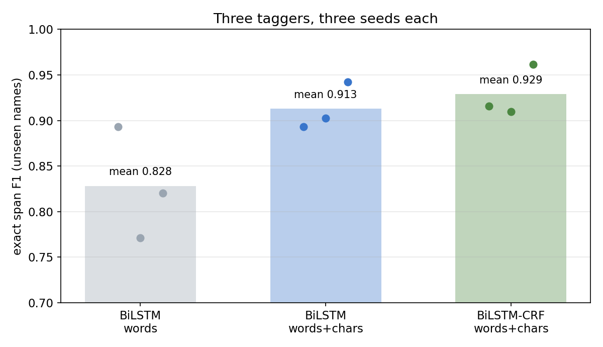
Reading the results
Character features fix detection. The word-only tagger sees most test names as the unknown id. Its errors are dominated by missed entities (247 over three seeds), plus boundary errors when a two-token name is split or truncated. With character features, misses drop to 7 and boundary errors to 2: the suffixes and capitalization of new names are enough to find them. Mean F1 rises from 0.828 to 0.913.
What remains is typing. Almost all remaining errors for both character models are type errors (124 and 102 over three seeds): the span is right but a person is labeled as an organization or the reverse. They involve single-token names, often in templates that accept either type in the same slot, such as Mimitek reported a fault or checked by Renaka. Context cannot settle those cases, the spelling of a person name carries no type marker in this corpus, and a model trained on 100 sentences has not learned the tek and corp endings reliably enough to override a context that also fits a person. This is the limit described in the character-features section: spelling helps only when it encodes the distinction.
The CRF guarantees valid output and helps a little. The word-only tagger produced 30 invalid I- tags in one seed and the character softmax tagger produced 4 and 1 in two seeds; the CRF with BIO constraints produced none, by construction. Its mean F1 is 0.929 against 0.913, and it is at least as good as the softmax tagger for each seed. With 100 training sentences that is a small margin; it is the consistency of the improvement and the guarantee of well-formed spans, not its size, that justifies the extra layer here.
Seeds matter again. The word-only tagger ranges from 0.771 to 0.893 across seeds. The seed with 30 invalid transitions is also the worst one. As in NLP 05, a single run would have been an unreliable summary.
What this does not show. The corpus is synthetic, tiny and templated; the test sentences reuse the training templates; and the tag set is small. Real benchmarks contain ambiguous context, nested and discontinuous mentions, and annotation disagreements. The experiment isolates three mechanisms (unknown-word handling, character evidence and output constraints) so that each effect can be seen and measured; it does not estimate how large those effects are on CoNLL-2003 or any other dataset.
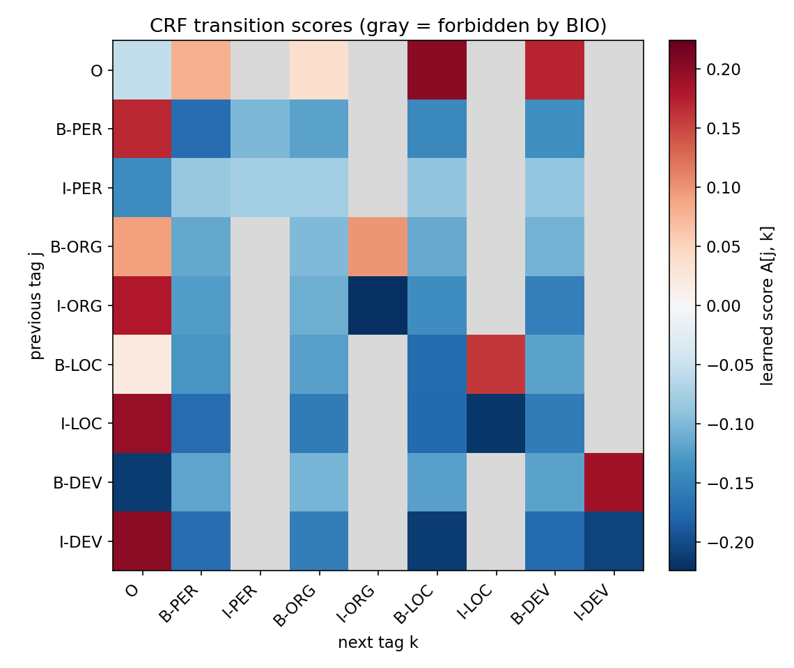
What the transitions learned. Figure 4 shows the learned transition scores for one seed. Inside the allowed region, the CRF has learned the corpus’s structure: B-LOC → I-LOC and B-DEV → I-DEV are strongly positive, while I-ORG → I-ORG and I-LOC → I-LOC are strongly negative, because no name in this corpus is longer than two tokens. A learned transition table is also a modeling assumption to inspect. Trained on a domain where every name has at most two tokens, it will penalize a three-token name elsewhere.
Modern view
Plain version. Current extraction systems combine pretrained representations with explicit task definitions. General language generation increases flexibility, while leaving span fidelity and support as separate problems.
Li and colleagues’ NER survey organizes earlier deep systems by input representation, context encoder and tag decoder [7]. This taxonomy is still useful: changing the encoder does not determine whether the output is a flat sequence or overlapping spans. Xu and colleagues’ 2024 generative extraction survey adds a task axis—entities, relations, events and unified extraction—and an adaptation axis including prompting, examples, supervised tuning and constrained generation [8]. Read these maps as design dimensions, rather than a ranking of universally superior architectures.
From BiLSTM-CRF to pretrained encoders. In Li and colleagues’ taxonomy, this chapter’s experiment varies the input representation (words versus words plus characters) and the tag decoder (softmax versus CRF) while keeping a BiLSTM context encoder [7]. Between 2016 and 2018 the BiLSTM-CRF with character features [14], [15] became the standard recipe, and contextual string embeddings from character language models extended it [16]. Pretrained Transformer encoders then replaced the BiLSTM as the context encoder in most systems; a linear or CRF tag decoder on top of them is the token-classification head discussed in NLP 10 and NLP 11. The decoder questions of this chapter (valid transitions, span boundaries, exact evaluation) carry over unchanged.
Large language models for open entity recognition. UniversalNER (ICLR 2024) distills a large language model into much smaller models for open-domain NER through targeted instruction tuning, and evaluates them on a benchmark assembled from 43 NER datasets across 9 domains [22]. Together with GLiNER [9], it represents a move from a fixed tag inventory to entity types supplied at inference time.
GLiNER is a 2024 original example of label-conditioned span extraction with a bidirectional Transformer [9]. Its design shows that adapting the requested entity categories need not require autoregressively generating a long list of records. A structured span output can retain direct alignment with input text. The relevant comparison for an application includes supported category definitions, nested-span behavior, latency and error review, alongside aggregate accuracy.
A generative extractor instead emits a textual serialization of the requested record. Enforcing a valid schema can prevent missing keys or malformed syntax, but valid serialization does not guarantee a correct name, relation or evidence interval. A practical validation layer checks that quoted evidence exists, offsets match, categories are allowed and entity identities are consistent. These checks eliminate some errors while leaving interpretation errors for evaluation or review.
Open problems include changing category inventories, specialized language, nested entities, cross-document identity and reliable uncertainty under domain shift. Multilingual extraction adds different name boundaries, writing systems and conventions for titles. Treat a language-specific annotation guideline as part of the task definition; translating category names is insufficient. Evaluate documents by source and language while keeping enough examples to make each comparison interpretable.
For a new project, establish a deterministic or compact supervised baseline, freeze an annotation guide and inspect its error types before choosing a larger model. Use a held-out document set that prevents repeated templates or near-duplicate reports crossing the split. Compare complete supported records, not only whether a model returns parseable output. The result is a measurable extraction service whose failures can be traced back to evidence.
New labels test both representation and interpretation
Label-conditioned span extraction [9] and generative extraction [8] change how an application supplies its category inventory. That flexibility creates an analytical question: does the model recognize the intended category, or merely react to a familiar label name? Compare a short label with a precise description and deliberately similar competing descriptions. For example, distinguish an equipment manufacturer from an equipment operator; both may be organization mentions, but their event roles differ.
Keep entity detection, requested typing and relation assignment as separate judgments. A correctly located organization span does not establish that it manufactured the device. Likewise, a generated record that fills every requested field may invent a participant when the source omitted it. Test an explicit unknown answer against forced completion. The comparison should reveal which output interface preserves missing information and which training examples distinguish closely related schemas. Broader category coverage is useful only when the semantic boundaries remain clear.
Key takeaways
- Sequence labeling assigns one label per token, but labels interact; a structured decoder chooses the best complete sequence under a stated factorization.
- HMM Viterbi decoding is exact for its first-order factorization; a linear-chain CRF keeps the same recursions while scoring tags conditionally, so a neural encoder can supply the scores.
- Entity recognition starts with a schema and offsets; BIO labels encode flat spans, and nested mentions need a span representation.
- Evaluate exact spans (boundaries and type), and break errors into missed, spurious, boundary and type errors instead of reporting token accuracy.
- A BiLSTM tagger reads the whole sentence in both directions; masks and trained unknown-word ids are essential details.
- A CRF layer trained by log-likelihood (forward algorithm) and decoded by Viterbi makes tags agree; BIO constraints make invalid sequences impossible.
- Character features recover unseen names from their spelling but cannot resolve ambiguity the spelling does not encode.
- Information extraction builds relations and events on top of entity spans; each layer adds its own record contract and failure modes.
Exercises
- A sequence decision. Change one transition row in the HMM while preserving its normalization. Find the condition under which the best path for “fish fish” becomes two nouns.
Hint
Compare the complete path products. The initial factor and first emission are shared by the two noun-initial candidates.
- Extend the CPU extraction example with a new person spelling that is absent from the inventory. Add its gold span and report the change in exact recall.
Hint
Keep the original inventory frozen. A missed mention is useful evidence about the baseline’s scope, rather than a reason to edit the test vocabulary into training.
- Design a schema for overlapping organization and department names. Explain why a single flat BIO sequence cannot express every allowed annotation.
Hint
Draw the character intervals first. Decide whether nested names count as separate entities and whether a department is linked to its parent organization.
- In the PyTorch experiment, remove the BIO constraint mask from the CRF (set
banandban_startto zeros) and retrain. Count invalidI-tags over three seeds, then inspect the learned transition scores forOfollowed byI-ORG.
Hint
Without the mask, invalid transitions are discouraged only to the extent the 100 training sentences teach it. Compare the learned score with the scores of allowed transitions into I-ORG.
- Add a character-only ablation: drop the word embedding and keep the character BiLSTM. Then give person names a distinctive ending in the generator (for example
-ko) and retrain all models. Which error type changes, and why?
Hint
Use the error breakdown printed by the script. A new spelling cue should move errors out of the type column only for the names that carry it.
- Write a partial-match evaluator that gives credit when a predicted span overlaps a gold span of the same type. Report it next to exact F1 for the word-only tagger and explain why the two can rank models differently.
Hint
Define the matching rule precisely (for example one-to-one matching by largest overlap) and report it under its own name. The word-only tagger’s boundary errors are where the two scores diverge.
References
- Susan McRoy, Principles of Natural Language Processing, open textbook, 2021; Chapters 3–5 and 8. Open textbook
- Masato Hagiwara, Real-World Natural Language Processing: Practical Applications with Deep Learning, Manning, 2021; Chapter 5, “Sequential labeling and language modeling.” Chapter
- L. R. Rabiner, “A tutorial on hidden Markov models and selected applications in speech recognition,” Proceedings of the IEEE, 77(2), 1989. Paper
- M.-C. de Marneffe, C. D. Manning, J. Nivre and D. Zeman, “Universal Dependencies,” Computational Linguistics, 47(2), 2021. Paper
- J. Lafferty, A. McCallum and F. Pereira, “Conditional random fields: Probabilistic models for segmenting and labeling sequence data,” ICML, 2001. Paper
- Erik F. Tjong Kim Sang and Fien De Meulder, “Introduction to the CoNLL-2003 Shared Task: Language-Independent Named Entity Recognition,” CoNLL, 2003. Paper
- Jing Li, Aixin Sun, Jianglei Han and Chenliang Li, “A Survey on Deep Learning for Named Entity Recognition,” IEEE Transactions on Knowledge and Data Engineering 34(1), 2022. Author-hosted paper
- Derong Xu, Wei Chen, Wenjun Peng, Chao Zhang, Tong Xu, Xiangyu Zhao, Xian Wu, Yefeng Zheng, Yang Wang and Enhong Chen, “Large language models for generative information extraction: a survey,” Frontiers of Computer Science 18(6), 2024. Survey
- Urchade Zaratiana, Nadi Tomeh, Pierre Holat and Thierry Charnois, “GLiNER: Generalist Model for Named Entity Recognition using Bidirectional Transformer,” NAACL, 2024. Paper
- Lance Ramshaw and Mitch Marcus, “Text Chunking using Transformation-Based Learning,” Third Workshop on Very Large Corpora, 1995. Paper
- Mitchell P. Marcus, Beatrice Santorini and Mary Ann Marcinkiewicz, “Building a Large Annotated Corpus of English: The Penn Treebank,” Computational Linguistics 19(2), 1993. Paper
- Ronan Collobert, Jason Weston, Léon Bottou, Michael Karlen, Koray Kavukcuoglu and Pavel Kuksa, “Natural Language Processing (Almost) from Scratch,” Journal of Machine Learning Research 12, 2011. Paper
- Zhiheng Huang, Wei Xu and Kai Yu, “Bidirectional LSTM-CRF Models for Sequence Tagging,” arXiv:1508.01991, 2015. arXiv
- Guillaume Lample, Miguel Ballesteros, Sandeep Subramanian, Kazuya Kawakami and Chris Dyer, “Neural Architectures for Named Entity Recognition,” NAACL-HLT, 2016. Paper
- Xuezhe Ma and Eduard Hovy, “End-to-end Sequence Labeling via Bi-directional LSTM-CNNs-CRF,” ACL, 2016. Paper
- Alan Akbik, Duncan Blythe and Roland Vollgraf, “Contextual String Embeddings for Sequence Labeling,” COLING, 2018. Paper
- Sameer Pradhan, Alessandro Moschitti, Nianwen Xue, Hwee Tou Ng, Anders Björkelund, Olga Uryupina, Yuchen Zhang and Zhi Zhong, “Towards Robust Linguistic Analysis using OntoNotes,” CoNLL, 2013. Paper
- Leon Derczynski, Eric Nichols, Marieke van Erp and Nut Limsopatham, “Results of the WNUT2017 Shared Task on Novel and Emerging Entity Recognition,” Workshop on Noisy User-generated Text, 2017. Paper
- Christopher Walker, Stephanie Strassel, Julie Medero and Kazuaki Maeda, ACE 2005 Multilingual Training Corpus, LDC2006T06, Linguistic Data Consortium, 2006. Catalog
- Yuhao Zhang, Victor Zhong, Danqi Chen, Gabor Angeli and Christopher D. Manning, “Position-aware Attention and Supervised Data Improve Slot Filling,” EMNLP, 2017. Paper
- Yuan Yao, Deming Ye, Peng Li, Xu Han, Yankai Lin, Zhenghao Liu, Zhiyuan Liu, Lixin Huang, Jie Zhou and Maosong Sun, “DocRED: A Large-Scale Document-Level Relation Extraction Dataset,” ACL, 2019. Paper
- Wenxuan Zhou, Sheng Zhang, Yu Gu, Muhao Chen and Hoifung Poon, “UniversalNER: Targeted Distillation from Large Language Models for Open Named Entity Recognition,” ICLR, 2024. arXiv
- Mike Schuster and Kuldip K. Paliwal, “Bidirectional Recurrent Neural Networks,” IEEE Transactions on Signal Processing 45(11), 1997. DOI
Check your understanding
This tutorial has 6 exercises. Can you solve them without opening the hints?
Go to the exercises ↑Next NLP 07 · Attention Mechanism and Transformers · 25 min