NLP 10 · Pretrained Models: BERT
Needs: NLP 09 · Language Modeling with Transformers (Natural Language Generation)
Navigate: this page and this track: Navigate: this page and this track
On this page
- What you’ll learn1 min
- The big picture1 min
- 1. Pretraining, then fine-tuning1 min
- 2. Masked and conditional objectives2 min
- 3. From text to BERT input2 min
- 4. The encoder1 min
- 5. What BERT learns before task labels are available2 min
- 6. A runnable bidirectional encoder1 min
- 7. Pretraining a tiny BERT from scratch2 min
- 8. Contextual versus static embeddings1 min
- 9. Probing what the representations contain2 min
- 10. The BERT family1 min
- 11. Multilingual and Chinese BERT2 min
- Modern view1 min
- Key takeaways1 min
- Exercises2 min
- Paper guides
- References
Natural Language Processing
Explore this chapter 2 interactive experiments
Change a right-context clue, hide it causally, then attach different output heads to the same small contextual vector.
What you’ll learn
- Explain the pretrain-then-fine-tune recipe and where BERT sits next to ELMo and GPT.
- Turn text into BERT input: WordPiece pieces,
[CLS]/[SEP]packing, and summed token, segment and position embeddings. - State the masked-language-modeling objective exactly (15% selection, 80/10/10 replacement), and the next-sentence-prediction objective with its later critique.
- Pretrain a tiny BERT-style encoder from scratch on a toy corpus, and measure what it learned.
- Distinguish contextual from static embeddings, and probe representations with a control task.
- Place RoBERTa, ALBERT, DistilBERT, ELECTRA, multilingual BERT and Chinese BERT models in one map.
The big picture
Standard Word2Vec features retrieve a fixed vector per word [6]. BERT, short for Bidirectional Encoder Representations from Transformers, computes a new representation for each token occurrence by reading its surrounding text [1]. In “the crane lifts steel” and “the crane eats fish,” the embedding lookup for crane is initially the same; the encoder can use the remaining words to produce different final vectors. The distinction is between a vocabulary entry and a representation of this occurrence.
BERT is learned in two stages. Pretraining uses ordinary unlabeled text, where the text supplies its own targets. Fine-tuning then adapts the same network, plus a small task head, to a labeled task such as sentiment or entailment. The first stage is expensive and done once; the second is cheap and done per task.
Hagiwara’s Chapter 9 develops pretrained-model adaptation in a practical setting [18]. This chapter goes inside the model. It reuses the causal language model of NLP 09 as a contrast, the attention block of NLP 07, and the static embeddings of NLP 04. The classification, entailment, tagging and extractive question-answering heads that sit on top of BERT are the subject of NLP 11. Every model here is tiny and trained from scratch; no checkpoint is downloaded.
1. Pretraining, then fine-tuning
Plain version. Learn general knowledge about language from a large amount of unlabeled text, then reuse it for a task with few labels. The question is what pretraining objective produces the most reusable representation.
Three 2018 designs frame BERT. ELMo trained left-to-right and right-to-left LSTM language models and supplied a learned combination of their internal states as contextual word features to existing task models [5]. GPT pretrained a 12-layer decoder-only Transformer as a left-to-right language model and then fine-tuned the whole network on each task [4]. BERT kept GPT’s fine-tune-everything recipe but replaced the causal objective with a masked one, so every layer can use both left and right context [1].
The BERT paper argues that the left-to-right constraint is sub-optimal for sentence-level tasks and can be very harmful for token-level tasks such as question answering, where context from both directions matters [1]. Its ablations include a left-to-right model without next sentence prediction, trained and fine-tuned under the same left-only constraint, and compare it with the bidirectional model [1]. The engineering lesson is that the visibility pattern is a modeling choice tied to the task, not a matter of taste.
Pretraining supplies an initialization and a representation function. It does not supply an application’s labels. A pump-maintenance classifier still needs examples defining “urgent,” and an entity tagger still needs examples identifying the site’s equipment names. Fine-tuning then adjusts the encoder and a task head together; freezing the encoder and training only the head is a cheaper alternative with a different adaptation capacity.
2. Masked and conditional objectives
Plain version. Not every pretrained language model predicts the next token. A masked objective uses surrounding context, while a conditional generator predicts an output sequence from a separate input.
BERT’s masked language objective hides selected input positions and predicts their original tokens using bidirectional context [1]. A simplified description is:
Here is the set of supervised masked positions; is its size; is the original token; denotes model parameters; and is the corrupted input sequence. The tilde indicates corruption, not an independently sampled document. This expression describes the masked prediction component; Section 5 gives the full corruption procedure.
A masked predictor is useful for contextual representations, classification and span-oriented tasks. Its loss is not automatically the log probability of an ordinary left-to-right sequence. Multiplying predictions that each use both sides of the sentence does not generally yield the same normalized joint distribution as a causal factorization. Consequently, masked-objective scores and causal perplexities are not directly interchangeable.
Conditional sequence generation instead writes:
Here is the source sequence; is the target sequence; is target length including any end token; and is the target prefix. The source can be visible in full while the target remains causal. T5 organizes many NLP tasks in a text-to-text framework and studies transfer learning with a Transformer encoder–decoder [27]; NLP 08 develops this family.
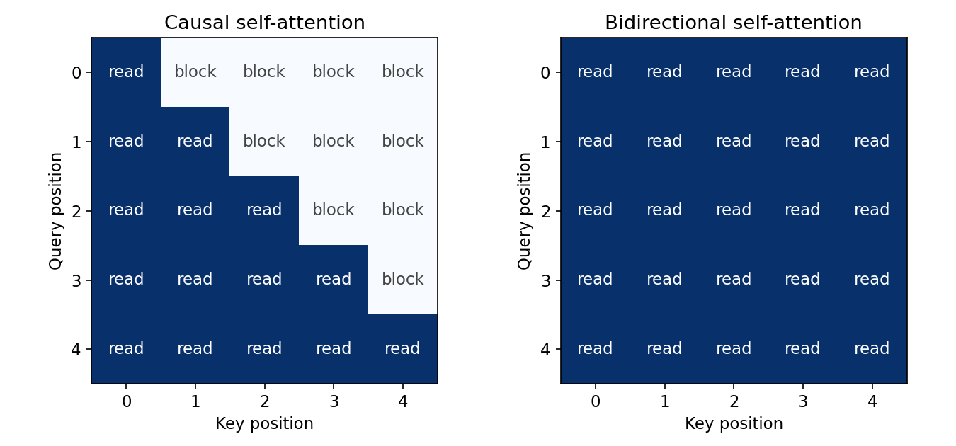
These distinctions guide model choice. A sentence classifier may use a bidirectional encoder because the complete sentence is available. A streaming continuation must exclude future output tokens. Translation can use the entire source after it arrives, but simultaneous translation needs a more restrictive source visibility contract. The task’s available information should determine the mask, rather than choosing a mask because a particular model name is familiar.
3. From text to BERT input
Plain version. BERT never sees words directly. Text is split into vocabulary pieces, wrapped with special markers, and each position receives the sum of three learned vectors.
WordPiece
The original tokenizer first applies text preprocessing, then WordPiece tokenization [2]. BERT uses WordPiece embeddings with a 30,000-token vocabulary [1], a subword method introduced for Google’s neural machine translation system [7]. WordPiece splits a word into vocabulary pieces when needed; ## marks a continuation piece in the original vocabulary convention. The original implementation splits each word greedily, longest match first: take the longest vocabulary entry that starts the word, then the longest continuation piece, and so on; if some remainder matches nothing, the whole word becomes [UNK] [2]. The vocabulary is learned beforehand from a corpus, as BPE merges are in NLP 02.
Code · Python · 34 lines
vocab = {'[UNK]', 'the', 'pump', 'over', 'heat', '##heat', '##ed', '##s',
         'un', '##load', 'load', '##ing', '幫', '浦', '過', '熱'}

def wordpiece(word, max_chars=200):
    """Greedy longest-match-first split into vocabulary pieces."""
    if len(word) > max_chars:
        return ['[UNK]']
    pieces, start = [], 0
    while start < len(word):
        end = len(word)
        while end > start:
            piece = word[start:end] if start == 0 else '##' + word[start:end]
            if piece in vocab:
                break
            end -= 1
        if end == start:                     # no piece fits: the whole word is unknown
            return ['[UNK]']
        pieces.append(piece)
        start = end
    return pieces

def basic_split(text):
    """Lowercase, put spaces around CJK ideographs, split on whitespace."""
    out = []
    for ch in text.lower():
        cjk = 0x4E00 <= ord(ch) <= 0x9FFF
        out.append(f' {ch} ' if cjk else ch)
    return ''.join(out).split()

for text in ['The pump overheated', 'unloading pumps', 'the pumpkin', '幫浦過熱']:
    tokens = [p for w in basic_split(text) for p in wordpiece(w)]
    print(f'{text!r:24} -> {tokens}')
assert wordpiece('overheated') == ['over', '##heat', '##ed']
assert wordpiece('pumpkin') == ['[UNK]']
Output:
Code · 4 lines
'The pump overheated'    -> ['the', 'pump', 'over', '##heat', '##ed']
'unloading pumps'        -> ['un', '##load', '##ing', 'pump', '##s']
'the pumpkin'            -> ['the', '[UNK]']
'幫浦過熱'                   -> ['幫', '浦', '過', '熱']
Three consequences follow. A word may occupy several model positions, so word labels and character spans must be mapped to token positions. A word whose remainder is not covered becomes a single [UNK], even though its prefix pump is known; that is a property of the greedy rule, not of the language. And Chinese characters are split one per position before WordPiece, as the original multilingual and Chinese models do (Section 11). The basic_split here checks only the main CJK Unified Ideographs block; the original code checks several more ranges and also handles accents and punctuation [2].
Pack one text or a text pair
For a single text, pack [CLS] text [SEP]. For a pair, pack [CLS] text A [SEP] text B [SEP]. [CLS] supplies a position whose final state can be read by a sequence classifier; [SEP] marks boundaries. Segment IDs distinguish the two parts. They do not block attention between them: a query in text A can read text B. This joint encoding is useful when a decision depends on their interaction [2].
Before the encoder, sum three learned vectors:
Here is packed sequence length; denotes encoder parameters; is the token ID at position ; is its segment ID; is the token table for vocabulary ; is the position table with supported length ; is the segment table; is the summed input; and contains contextual output rows . The original implementation normalizes and applies dropout to the summed embeddings [2]. Padding keys are blocked; ordinary text on either side remains visible.
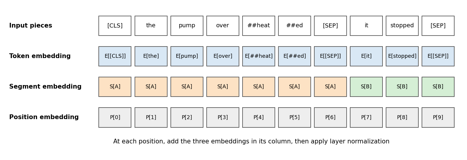
Unlike the fixed sinusoids of the original Transformer, BERT’s position vectors are learned rows [2]. A learned position table imposes a maximum supported position; a longer input is an invalid lookup, not an ordinary longer sequence, and must be truncated or split into windows. Embedding rows also have meaning only relative to the model’s token IDs. Swapping in a different tokenizer without adapting weights can turn apparently valid numbers into unrelated symbols.
4. The encoder
Plain version. BERT is the encoder half of a Transformer: a stack of identical blocks, each letting every position read every other position and then transforming each position separately.
BERT is a stack of Transformer encoder blocks [1, 3]. Each block mixes information with bidirectional self-attention, then transforms each position with a feedforward network; residual connections and layer normalization support the stack [9]. “Bidirectional” means both left and right input positions are available throughout the encoder. It does not mean training two separate causal models and joining their outputs, as ELMo does [5]. NLP 07 derives multi-head attention; the only BERT-specific choice is the attention mask of Figure 1.
The paper reports two sizes. Writing for the number of blocks, for the hidden width and for attention heads, BERT-Base has , , and 110M parameters, and BERT-Large has , , and 340M parameters [1]. BERT-Base was chosen to match the size of the original GPT for comparison [1]. The feedforward layers use the GELU activation [8, 1]. Pretraining used BooksCorpus and English Wikipedia, and the paper stresses using a document-level corpus so that long contiguous sequences are available [1].
Think of the outputs as a table with one row per input token, rather than a single sentence vector. A token-labeling head reads those rows individually. A sequence head reads the first row through a pooling transformation. The same encoder can support both because its output preserves token positions; NLP 11 builds those heads.
5. What BERT learns before task labels are available
Plain version. Masked language modeling turns raw text into a fill-in-the-blank exercise. Next sentence prediction adds a yes/no question about whether two text segments belong together.
Masked language modeling
Masked language modeling (MLM) learns from ordinary text: the original tokens provide their own targets. For example, the crane [MASK] steel asks the model to predict the removed token using words on both sides. The prediction loss updates the encoder as well as the vocabulary head, so the final token vectors become useful inputs for later supervised tasks.
Original BERT selects 15% of WordPiece positions as prediction targets. Among selected positions, it inserts [MASK] 80% of the time, a random token 10%, and leaves the original token unchanged 10% [1]. Selection and replacement are different: every selected position contributes a target, even when its visible token is unchanged. Other positions supply context without contributing MLM loss. This mixed replacement reduces the difference between pretraining inputs and ordinary unmasked task inputs, where [MASK] never appears.
The price of this design is sample efficiency: only the selected positions produce a loss. ELECTRA’s authors make exactly this point, noting that MLM learns from only the masked subset of tokens per example [14]. The original implementation also chose masks once when the data was prepared; RoBERTa compared that static masking with dynamic masking, which draws a new pattern every time a sequence is used, and found dynamic masking comparable or slightly better [11]. The tiny model in Section 7 masks dynamically.
Next sentence prediction and its critique
Original BERT also trains next sentence prediction (NSP) [1]: a text pair is either consecutive corpus text or a pair whose second segment is sampled from the corpus, with equal sampling probability. The pooled [CLS] state predicts this binary label. NSP predicts a relationship label; it does not generate the next sentence. The original pretraining objective combines MLM and NSP, and the paper’s ablation reported that removing NSP hurt performance on QNLI, MNLI and SQuAD 1.1 [1].
Later work disagreed. RoBERTa’s replication study found that removing the NSP loss matches or slightly improves downstream performance when inputs are filled with contiguous text, and suggested that the original ablation may have removed the loss while keeping the segment-pair input format [11]. ALBERT’s authors conjectured that NSP is too easy because it conflates topic prediction with coherence prediction: a randomly sampled second segment usually differs in topic. They replaced it with sentence-order prediction, which uses two consecutive segments from the same document either in order or swapped, so topic no longer gives the answer away [12]. The general lesson is to inspect a checkpoint’s actual objectives rather than assume every later encoder keeps every original design choice.
Optional: BERT (in the Paper guides). Follow the original figure, objective, experimental comparisons and limitations.
6. A runnable bidirectional encoder
Plain version. Before pretraining a whole model, isolate the two properties that make it BERT-like: changing a later word changes an earlier word’s representation, and padding changes nothing.
The following CPU example trains MLM on four invented sentences. Position 2 is always selected and replaced with [MASK], making the visible right-hand verb useful for distinguishing robot from sensor. This deliberately simpler corruption policy isolates the mechanism; the model is randomly initialized, has one small encoder block, and uses a linear vocabulary head rather than reproducing original BERT’s full head. It uses layer normalization, GELU and AdamW [8–10].
Code · Python · 68 lines
import torch
from torch import nn
from torch.nn import functional as F

torch.manual_seed(23)
torch.set_num_threads(1)
vocab = ['[PAD]', '[CLS]', '[SEP]', '[MASK]', 'the', 'a',
         'robot', 'sensor', 'moves', 'measures']
index = {word: i for i, word in enumerate(vocab)}
rows = ['the robot moves', 'the sensor measures',
        'a robot moves', 'a sensor measures']
ids = torch.tensor([[index[w] for w in ['[CLS]'] + s.split()
                     + ['[SEP]', '[PAD]']] for s in rows])
blocked = ids.eq(index['[PAD]'])
corrupted = ids.clone()
corrupted[:, 2] = index['[MASK]']
labels = torch.full_like(ids, -100)
labels[:, 2] = ids[:, 2]

class TinyEncoder(nn.Module):
    def __init__(self):
        super().__init__()
        self.word = nn.Embedding(len(vocab), 16)
        self.position = nn.Embedding(6, 16)
        self.segment = nn.Embedding(2, 16)
        self.embed_norm = nn.LayerNorm(16)
        self.layer = nn.TransformerEncoderLayer(
            16, 2, 32, dropout=0.0, activation='gelu', batch_first=True)
        self.mlm = nn.Linear(16, len(vocab))
        self.pool = nn.Sequential(nn.Linear(16, 16), nn.Tanh())
        self.classifier = nn.Linear(16, 3)
        self.tagger = nn.Linear(16, 3)
        self.span = nn.Linear(16, 2)
    def forward(self, tokens, padding):
        positions = torch.arange(tokens.shape[1])
        segments = torch.zeros_like(tokens)  # single segment here
        h = self.embed_norm(self.word(tokens) + self.position(positions)
                            + self.segment(segments))
        return self.layer(h, src_key_padding_mask=padding)

model = TinyEncoder()
optimizer = torch.optim.AdamW(model.parameters(), lr=0.01)
def objective():
    logits = model.mlm(model(corrupted, blocked))
    return F.cross_entropy(logits.reshape(-1, len(vocab)), labels.reshape(-1))
initial = objective().item()
for _ in range(100):
    optimizer.zero_grad()
    loss = objective()
    loss.backward()
    optimizer.step()
model.eval()
with torch.no_grad():
    final = objective().item()
    h = model(ids, blocked)
    changed = ids.clone()
    changed[0, 3] = index['measures']
    context_gap = (model(changed, blocked)[0, 2] - h[0, 2]).abs().max().item()
    changed_padding = ids.clone()
    changed_padding[blocked] = index['robot']
    pad_gap = (model(changed_padding, blocked)[~blocked] - h[~blocked]).abs().max().item()
    shapes = [model.classifier(model.pool(h[:, 0])).shape,
              model.tagger(h).shape, model.span(h).shape]
assert final < initial and context_gap > 1e-4 and pad_gap < 1e-6
print('masked loss:', round(initial, 3), '->', round(final, 3))
print('context changes representation:', context_gap > 1e-4)
print('padding leaves real tokens unchanged:', pad_gap < 1e-6)
print('class / tag / span shapes:', [tuple(s) for s in shapes])
Output:
Code · 4 lines
masked loss: 2.223 -> 0.001
context changes representation: True
padding leaves real tokens unchanged: True
class / tag / span shapes: [(4, 3), (4, 6, 3), (4, 6, 2)]
The masked loss falls from 2.223 to 0.001. This measures fitting those four examples. Changing the word after robot changes its final representation, whereas changing the value stored at blocked padding positions leaves real-token outputs unchanged. A causal model must reject the first kind of future influence (the perturbation test of NLP 09); a bidirectional encoder deliberately allows it.
The task heads print shapes (4, 3), (4, 6, 3) and (4, 6, 2): four sequence decisions over three categories, six token decisions per example, and two boundary scores per token. Those heads are untrained. Only the encoder and MLM head receive gradients in this example. To build an application, supply its labels, optimize the corresponding head and encoder, and evaluate held-out task outputs, as NLP 11 does.
There are two masks to keep separate. The encoder’s padding mask controls readable keys. The -100 labels tell cross-entropy which positions to ignore; they do not remove those positions from attention. In the demonstration, all real words may provide context, but only the selected noun contributes MLM loss.
7. Pretraining a tiny BERT from scratch
Plain version. Now apply the real corruption recipe to a small artificial language, train for a few seconds, and check three things: how well the model fills in held-out blanks, whether one word gets different vectors in different contexts, and what simple classifiers can read from each layer.
The toy corpus comes from a small grammar. The subject constrains the verb and the verb constrains the object, so a masked word is often predictable from both sides. The word crane is deliberately ambiguous: it can lift (a machine) or eat (a bird). Of the 128 possible sentences, 40 are held out. The corruption function implements Section 5 exactly: 15% selection, then 80/10/10 replacement, with a fresh draw on every step.
Code · Python · 137 lines
import itertools, random
from collections import Counter
import numpy as np
import torch
from torch import nn
from torch.nn import functional as F
from sklearn.linear_model import LogisticRegression
from sklearn.model_selection import cross_val_score

random.seed(0); torch.manual_seed(0); torch.set_num_threads(1)

# 1. A toy corpus: the subject constrains the verb, the verb constrains the object.
frames = {'robot': ['lifts', 'moves'], 'crane': ['lifts', 'eats'],
          'technician': ['repairs', 'moves'], 'heron': ['eats', 'sees']}
objects = {'lifts': ['steel', 'box'], 'moves': ['box', 'cart'],
           'eats': ['fish', 'bread'], 'repairs': ['pump', 'cart'], 'sees': ['fish', 'boat']}
sentences = [f'{d1} {a}{s} {v} {d2} {o}'.split()
             for s in frames for v in frames[s] for o in objects[v]
             for d1, d2, a in itertools.product(['the', 'a'], ['the', 'a'], ['', 'old '])]
random.shuffle(sentences)
test, train = sentences[:40], sentences[40:]
special = ['[PAD]', '[CLS]', '[SEP]', '[MASK]']
words = sorted({w for s in sentences for w in s})
vocab = special + words
index = {w: i for i, w in enumerate(vocab)}
first_word = len(special)
L = 2 + max(len(s) for s in sentences)

def encode(rows):
    ids = torch.zeros(len(rows), L, dtype=torch.long)
    for r, s in enumerate(rows):
        seq = [index['[CLS]']] + [index[w] for w in s] + [index['[SEP]']]
        ids[r, :len(seq)] = torch.tensor(seq)
    return ids
train_ids, test_ids = encode(train), encode(test)

# 2. BERT-style corruption: select 15% of real word positions; of those,
#    80% -> [MASK], 10% -> random word, 10% -> unchanged. All selected are targets.
def corrupt(ids, generator):
    real = ids >= first_word
    selected = (torch.rand(ids.shape, generator=generator) < 0.15) & real
    labels = torch.where(selected, ids, torch.full_like(ids, -100))
    u = torch.rand(ids.shape, generator=generator)
    out = ids.clone()
    out[selected & (u < 0.8)] = index['[MASK]']
    swap = selected & (u >= 0.8) & (u < 0.9)
    out[swap] = torch.randint(first_word, len(vocab), (int(swap.sum()),), generator=generator)
    return out, labels

class TinyBERT(nn.Module):
    def __init__(self, d=32, layers=2):
        super().__init__()
        self.word, self.position = nn.Embedding(len(vocab), d), nn.Embedding(L, d)
        self.segment, self.norm = nn.Embedding(2, d), nn.LayerNorm(d)
        self.blocks = nn.ModuleList(nn.TransformerEncoderLayer(
            d, 4, 4 * d, dropout=0.0, activation='gelu', batch_first=True)
            for _ in range(layers))
        self.mlm = nn.Linear(d, len(vocab))
    def forward(self, ids):
        pad = ids.eq(index['[PAD]'])
        h = self.norm(self.word(ids) + self.position(torch.arange(ids.shape[1]))
                      + self.segment(torch.zeros_like(ids)))
        states = [h]
        for block in self.blocks:
            h = block(h, src_key_padding_mask=pad)
            states.append(h)
        return states                               # embeddings, layer 1, layer 2

model = TinyBERT()
optimizer = torch.optim.AdamW(model.parameters(), lr=3e-3)
g = torch.Generator().manual_seed(1)
for step in range(600):                             # a fresh mask every step
    inputs, labels = corrupt(train_ids, g)
    logits = model.mlm(model(inputs)[-1])
    loss = F.cross_entropy(logits.reshape(-1, len(vocab)), labels.reshape(-1))
    optimizer.zero_grad(); loss.backward(); optimizer.step()
model.eval()

# 3. Held-out masked-word accuracy: mask each word position in turn.
def masked_hits(ids, rows_text):
    by_kind = {}
    with torch.no_grad():
        for r, s in enumerate(rows_text):
            for i, w in enumerate(s):
                x = ids[r:r + 1].clone(); x[0, i + 1] = index['[MASK]']
                guess = vocab[model.mlm(model(x)[-1][0, i + 1]).argmax()]
                kind = 'determiner/adjective' if w in ('the', 'a', 'old') else 'noun/verb'
                by_kind.setdefault(kind, []).append(guess == w)
    return {k: round(float(np.mean(v)), 3) for k, v in sorted(by_kind.items())}
counts = torch.bincount(train_ids[train_ids >= first_word], minlength=len(vocab))
real_test = test_ids[test_ids >= first_word]
print('final training MLM loss:', round(loss.item(), 3))
print('held-out masked accuracy:', masked_hits(test_ids, test))
print('most-frequent-word baseline:', vocab[int(counts.argmax())],
      round((real_test == counts.argmax()).float().mean().item(), 3))
# Upper reference: the best guess given every other word, read off the grammar.
def oracle(text):
    by_kind = {}
    for s in text:
        for i, w in enumerate(s):
            fits = Counter(t[i] for t in sentences if len(t) == len(s)
                           and all(a == b for j, (a, b) in enumerate(zip(t, s)) if j != i))
            kind = 'determiner/adjective' if w in ('the', 'a', 'old') else 'noun/verb'
            by_kind.setdefault(kind, []).append(fits[w] / sum(fits.values()))
    return {k: round(float(np.mean(v)), 3) for k, v in sorted(by_kind.items())}
print('expected accuracy of an ideal guesser:', oracle(test))

# 4. One word, two contexts: identical input row, different output rows.
with torch.no_grad():
    pair = encode([['the', 'crane', 'lifts', 'the', 'steel'],
                   ['the', 'crane', 'eats', 'the', 'fish']])
    cos = [F.cosine_similarity(s[0, 2], s[1, 2], dim=0).item() for s in model(pair)]
print('cosine of the two "crane" vectors by layer:', [round(c, 3) for c in cos])

# 5. Probes. (a) Part of speech vs a control task that gives each word type a
#    random label; (b) the sense of "crane" (machine vs bird) from its own vector.
pos = {w: 'DET' if w in ('the', 'a') else 'ADJ' if w == 'old' else
       'VERB' if w in objects else 'NOUN' for w in words}
control = {w: random.randint(0, 3) for w in words}
crane = [s for s in sentences if 'crane' in s]
crane_ids = encode(crane)
sense = np.array([int('eats' in s) for s in crane])
def rows(ids, text, layer):
    with torch.no_grad():
        h = model(ids)[layer]
    return np.array([h[r, i + 1].numpy() for r, s in enumerate(text) for i in range(len(s))])
for layer in range(3):
    Xtr, Xte = rows(train_ids, train, layer), rows(test_ids, test, layer)
    acc = []
    for table in (pos, control):
        ytr = [table[w] for s in train for w in s]; yte = [table[w] for s in test for w in s]
        acc.append(LogisticRegression(max_iter=3000).fit(Xtr, ytr).score(Xte, yte))
    h = model(crane_ids)[layer].detach()[:, :, :]
    Xc = np.array([h[r, s.index('crane') + 1].numpy() for r, s in enumerate(crane)])
    acc.append(cross_val_score(LogisticRegression(max_iter=3000), Xc, sense, cv=4).mean())
    print(f'layer {layer}: POS {acc[0]:.2f}  control {acc[1]:.2f}  crane sense {acc[2]:.2f}')
assert cos[0] > 0.999 and cos[-1] < cos[0]
Output (about six seconds on one CPU thread):
Code · 8 lines
final training MLM loss: 0.453
held-out masked accuracy: {'determiner/adjective': 0.418, 'noun/verb': 0.492}
most-frequent-word baseline: the 0.17
expected accuracy of an ideal guesser: {'determiner/adjective': 0.592, 'noun/verb': 0.633}
cosine of the two "crane" vectors by layer: [1.0, 0.819, 0.639]
layer 0: POS 1.00  control 1.00  crane sense 0.38
layer 1: POS 1.00  control 1.00  crane sense 1.00
layer 2: POS 1.00  control 1.00  crane sense 1.00
Read the masked-word numbers against two references. Always guessing the most frequent word, the, is right 17% of the time. An ideal guesser that knows the grammar exactly, and therefore the true distribution of each blank given every other word, would be right 63% of the time on content words, not 100%: after the robot ___ the box, both lifts and moves are grammatical. The model reaches 49% on content words from 88 training sentences. That gap is the honest measure of what it has and has not learned. Many blanks have no single answer, which is why MLM accuracy is never a direct measure of understanding.
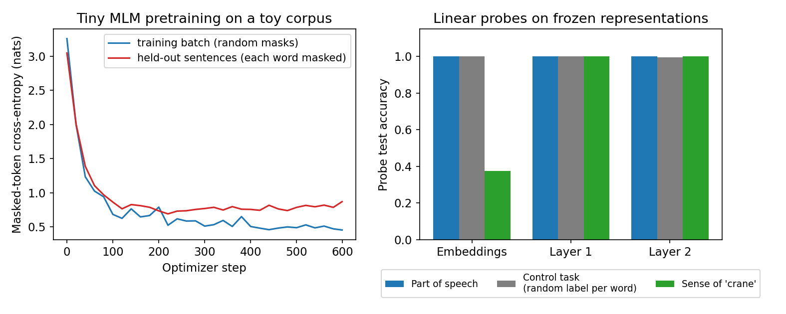
The left panel of Figure 3 shows the held-out loss flattening, then drifting up, while the training loss keeps falling. The same script trained for more steps lowers training loss further but makes held-out masked accuracy worse, so the 600-step budget was set by watching held-out loss, not training loss. That is ordinary model selection, and it applies to pretraining as much as to fine-tuning.
8. Contextual versus static embeddings
Plain version. A static embedding gives a word one vector everywhere. A contextual encoder gives each occurrence its own vector, and the difference grows with depth.
A Word2Vec or PPMI vector, as built in NLP 04, is a single row of a table: the bird and the machine share one crane vector, which must average their contexts. The printed cosines above show the contextual alternative in miniature. At the embedding layer, the two crane vectors are identical (cosine 1.0) because the token and its position are the same. After one encoder block the cosine is 0.819, and after two it is 0.639: the right-hand context lifts the steel or eats the fish has been mixed in.
Ethayarajh measured this effect in real models. In ELMo, BERT and GPT-2, representations of the same word in different contexts are still more similar than those of two different words, but this self-similarity is much lower in upper layers, and on average less than 5% of the variance in a word’s contextual representations can be explained by a static embedding for that word [19]. The same study found that contextual representations are not isotropic in any layer: vectors occupy a narrow region of the space [19]. A practical consequence is that raw cosine similarity between BERT vectors is not automatically a meaningful semantic similarity. Sentence-level similarity needs its own training objective, which NLP 04 and NLP 11 discuss.
Static vectors still have uses: they are cheap, need no encoder at inference time and are easy to inspect. Contextual vectors are preferable when the same surface form carries different meanings or roles, which is most of the time in real text.
9. Probing what the representations contain
Plain version. A probe is a small classifier trained on frozen representations to predict a linguistic property. If it succeeds, the property is recoverable from the vectors. Whether it was the representation or the probe that did the work is a separate question.
Tenney, Das and Pavlick probed BERT layer by layer and found that the regions responsible for part-of-speech tagging, parsing, named entities, semantic roles and coreference appear in roughly the order of the classical NLP pipeline, with later layers sometimes revising earlier decisions [20]. Hewitt and Manning’s structural probe looks for a linear transformation under which squared distances between word vectors encode distances in the parse tree, and found such transformations for ELMo and BERT but not for baselines [21]. Clark and colleagues analyzed attention instead of vectors and found heads that attend to delimiter tokens, to fixed positional offsets, and to direct objects, determiners and coreferent mentions [23].
Hewitt and Liang added the essential control. A control task assigns each word type a random label, so it can be solved only by memorizing word identities. A good probe should be selective: high accuracy on the linguistic task and low accuracy on its control [22]. Without that comparison, a high probe accuracy may show that the probe is powerful, not that the representation encodes the property.
Our tiny run illustrates both sides. Part of speech is perfectly recoverable at every layer, but so is a random label per word, because in this grammar part of speech is a function of the word itself. The probe’s success therefore says nothing beyond “the word is identifiable,” and its selectivity is zero. The crane sense probe is different. It is at chance or below (0.38, from 32 sentences in four folds) at the embedding layer, where both senses share one vector, and perfect after one encoder block. That property requires context, so the layer-wise rise is evidence that the encoder moved the information into the crane vector. Even so, a probe shows that information is available to a linear reader, not that the model uses it for its predictions.
10. The BERT family
Plain version. After BERT, several papers changed one part of the recipe at a time: how long to train, how to share parameters, how to compress, and what to predict.
| Model | What changed | Reported motivation |
|---|---|---|
| RoBERTa [11] | Longer training with bigger batches on more data, NSP removed, longer sequences, dynamic masking | A replication study finding BERT significantly undertrained |
| ALBERT [12] | Factorized embedding parameterization, cross-layer parameter sharing, sentence-order prediction | Lower memory and faster training; a coherence objective instead of NSP |
| DistilBERT [13] | Knowledge distillation during pretraining into a smaller student, with a triple loss | 40% smaller, retaining 97% of BERT’s language understanding and 60% faster, as reported by its authors |
| ELECTRA [14] | Replaced-token detection: a small generator fills masked positions, and the encoder classifies every token as original or replaced | Learning from all input tokens instead of only the masked subset |
ALBERT’s factorized embedding separates vocabulary size from hidden size: instead of one table it uses a table followed by an projection, with much smaller than [12]. Its authors argue that WordPiece embeddings are meant to be context-independent while hidden states are context-dependent, so the two sizes need not match [12]. ELECTRA’s discriminator is the model kept for fine-tuning; the generator is discarded after pretraining [14].
These variants change parameter counts, compute budgets and objectives together, so their published comparisons belong to their own experimental settings. When choosing one, check its tokenizer, maximum length, objectives and training data, and measure on the task you care about.
11. Multilingual and Chinese BERT
Plain version. One encoder can be pretrained on many languages at once with a shared vocabulary. Chinese needs a decision about units, because it is not written with spaces between words.
The original release includes a multilingual BERT-Base trained on the Wikipedias of 104 languages with a shared 110k WordPiece vocabulary and no marker telling the model which language it is reading [2]. Pires, Schlinger and Garrette found that this model transfers surprisingly well zero-shot, where a task is fine-tuned in one language and evaluated in another, including across scripts, and that transfer works best between typologically similar languages; they also found systematic deficiencies for certain language pairs [15]. XLM-R later trained a Transformer masked language model on one hundred languages with far more filtered CommonCrawl data and reported large gains over multilingual BERT on cross-lingual benchmarks, especially for low-resource languages [16]. Its analysis of the trade-off between positive transfer and capacity dilution is a reminder that adding languages to a fixed-size model is not free [16].
For Chinese, the original multilingual model adds spaces around every character in the CJK ideograph ranges before WordPiece, so Chinese is effectively character-tokenized [2]; the basic_split function in Section 3 imitates this rule. The release also provides a Chinese-only BERT-Base that covers both Simplified and Traditional Chinese [2]. Character positions avoid word-segmentation errors, but masking a single character of a multi-character word such as 幫浦 lets the model recover it from its partner character rather than from sentence context. Cui and colleagues introduced whole word masking for Chinese BERT: a word segmenter identifies word boundaries, and all characters of a selected word are masked together, while the input is still tokenized by characters [17]. Their MacBERT model replaces [MASK] with similar words chosen by word-vector similarity, reducing the gap between pretraining and fine-tuning inputs [17].
For Traditional Chinese text from Taiwan, check what the pretraining corpus actually contained, not only the language label. A model whose data is dominated by Simplified Chinese can tokenize Traditional characters correctly and still be weaker on regional vocabulary such as 資料 versus other usages, or on Taiwanese terminology in a domain. That is a data question to measure with in-domain examples, not something the architecture decides.
Modern view
Rogers, Kovaleva and Rumshisky’s primer [24] surveys over 150 studies of BERT: what linguistic and world knowledge it captures and where, how its attention heads and layers behave, modifications to its objectives and architecture, overparameterization and compression. Its overall message matches Section 9: many properties are recoverable, but recoverable is not the same as used, and probing results depend on the probe.
Encoders have not disappeared in the era of large decoder-only models. ModernBERT [25], published at ACL 2025, is a 2024 encoder-only model that brings recent architectural and efficiency optimizations to the BERT design; its authors describe encoders as the workhorse of many production retrieval and classification pipelines and report training on 2 trillion tokens with a native sequence length of 8,192. Zhao and colleagues’ survey [26] places masked encoders within the broader history of pretrained language models and notes that causal decoders have been widely adopted as the architecture of existing large language models; NLP 09 shows why one causal objective can serve both scoring and generation.
A practical 2026 summary: use a bidirectional encoder when the whole input is available and the output is a label, a span or a vector for retrieval, and when latency and cost matter; use a decoder-only model when the output is open-ended text. Open problems include faithful interpretation beyond probing, robust multilingual coverage for low-resource languages and scripts, long-document encoding beyond learned position limits, and evaluating how much a pretrained representation, rather than the fine-tuning data, explains a task result.
Key takeaways
- BERT is a Transformer encoder pretrained without labels and then fine-tuned with a small task head; pretraining supplies a representation, not task labels.
- Input is WordPiece pieces packed as
[CLS] A [SEP] B [SEP], with summed token, segment and learned position embeddings; segments do not block attention. - MLM selects 15% of positions and replaces them 80/10/10; every selected position is a target, and masked scores are not causal perplexities.
- NSP was later found unnecessary (RoBERTa) or replaced by sentence-order prediction (ALBERT).
- A tiny BERT pretrained from scratch shows the mechanisms: held-out blanks are filled better than a frequency baseline but below the grammar’s own ceiling, and an ambiguous word’s vectors diverge with depth.
- Contextual vectors differ by occurrence; static vectors do not. Raw cosine between contextual vectors is not automatically a semantic similarity.
- Probes need control tasks; a probe shows information is available, not that the model uses it.
- Multilingual and Chinese BERT models make specific unit choices (shared WordPiece, per-character CJK splitting, whole word masking) that affect what is learned.
Exercises
- In the tiny BERT, replace dynamic masking with a single static mask drawn once before training. Compare held-out masked accuracy and the loss curves.
Hint
Draw corrupt(train_ids, g) once outside the loop. With a static mask, each sentence always hides the same positions, so many (sentence, position) targets are never seen.
- Add next sentence prediction to the toy corpus: build pairs of two sentences joined by
[SEP]with segment IDs, where half the second sentences are random. Then build a sentence-order version. Which one can be solved from topic cues alone in your corpus?
Hint
Make two “documents” that use different vocabularies. A random second sentence then usually comes from the other document, so NSP is easy; swapped order within one document is not.
- Extend the WordPiece vocabulary so that
pumpkinis not[UNK], without addingpumpkinitself. Then find a word for which greedy longest-match gives a different split from the one with the fewest pieces.
Hint
Adding ##kin is enough for the first part. For the second, include a long prefix that leaves an awkward remainder, and a shorter prefix that leads to a clean split.
- Design a probing task on the toy corpus for which part-of-speech style control results would show positive selectivity. What property must depend on context rather than on word identity?
Hint
Subject versus object role of a noun is one option, but check first whether position alone already reveals it in this grammar. If it does, add sentence variants that break the link.
- Replace the MLM head with an ELECTRA-style replaced-token detector: corrupt positions with random words instead of
[MASK], and train a binary classifier on every position. Compare how many positions produce a loss per batch.
Hint
ELECTRA uses a small trained generator; random replacements make detection much easier, so say what your simplification changes. Count labeled positions with and without masking.
- Turn the bidirectional example into a token classifier. If one annotated word splits into three pieces, define which positions contribute to loss and how you reconstruct the word label.
Hint
Decide between first-piece supervision and an explicitly defined all-piece label mapping. Ignore padding and special markers, train the tag head, and map the output back to the original text.
References
- Jacob Devlin, Ming-Wei Chang, Kenton Lee and Kristina Toutanova, “BERT: Pre-training of Deep Bidirectional Transformers for Language Understanding,” NAACL, 2019. Paper
- Google Research, BERT: original implementation and released models, software, 2018. Encoder and pooler · Tokenizer · Multilingual and Chinese models
- Ashish Vaswani et al., “Attention Is All You Need,” NeurIPS, 2017. Paper
- Alec Radford, Karthik Narasimhan, Tim Salimans and Ilya Sutskever, “Improving Language Understanding by Generative Pre-Training,” OpenAI technical report, 2018. Paper
- Matthew E. Peters, Mark Neumann, Mohit Iyyer, Matt Gardner, Christopher Clark, Kenton Lee and Luke Zettlemoyer, “Deep Contextualized Word Representations,” NAACL, 2018. Paper
- Tomas Mikolov, Kai Chen, Greg Corrado and Jeffrey Dean, “Efficient Estimation of Word Representations in Vector Space,” ICLR Workshop, 2013. Paper
- Yonghui Wu et al., “Google’s Neural Machine Translation System: Bridging the Gap between Human and Machine Translation,” arXiv:1609.08144, 2016. Paper
- Dan Hendrycks and Kevin Gimpel, “Gaussian Error Linear Units (GELUs),” arXiv:1606.08415, 2016, revised 2023. Paper
- Jimmy Lei Ba, Jamie Ryan Kiros and Geoffrey E. Hinton, “Layer Normalization,” arXiv:1607.06450, 2016. Paper
- Ilya Loshchilov and Frank Hutter, “Decoupled Weight Decay Regularization,” ICLR, 2019. Paper
- Yinhan Liu et al., “RoBERTa: A Robustly Optimized BERT Pretraining Approach,” arXiv:1907.11692, 2019. Paper
- Zhenzhong Lan, Mingda Chen, Sebastian Goodman, Kevin Gimpel, Piyush Sharma and Radu Soricut, “ALBERT: A Lite BERT for Self-supervised Learning of Language Representations,” ICLR, 2020. Paper
- Victor Sanh, Lysandre Debut, Julien Chaumond and Thomas Wolf, “DistilBERT, a distilled version of BERT: smaller, faster, cheaper and lighter,” 5th Workshop on Energy Efficient Machine Learning and Cognitive Computing at NeurIPS, 2019. Paper
- Kevin Clark, Minh-Thang Luong, Quoc V. Le and Christopher D. Manning, “ELECTRA: Pre-training Text Encoders as Discriminators Rather Than Generators,” ICLR, 2020. Paper
- Telmo Pires, Eva Schlinger and Dan Garrette, “How Multilingual is Multilingual BERT?,” ACL, 2019. Paper
- Alexis Conneau et al., “Unsupervised Cross-lingual Representation Learning at Scale,” ACL, 2020. Paper
- Yiming Cui, Wanxiang Che, Ting Liu, Bing Qin and Ziqing Yang, “Pre-Training With Whole Word Masking for Chinese BERT,” IEEE/ACM Transactions on Audio, Speech, and Language Processing 29, 2021. Publisher · Author manuscript
- Masato Hagiwara, Real-World Natural Language Processing: Practical Applications with Deep Learning, Chapter 9, Manning, 2021. Publisher
- Kawin Ethayarajh, “How Contextual are Contextualized Word Representations? Comparing the Geometry of BERT, ELMo, and GPT-2 Embeddings,” EMNLP-IJCNLP, 2019. Paper
- Ian Tenney, Dipanjan Das and Ellie Pavlick, “BERT Rediscovers the Classical NLP Pipeline,” ACL, 2019. Paper
- John Hewitt and Christopher D. Manning, “A Structural Probe for Finding Syntax in Word Representations,” NAACL, 2019. Paper
- John Hewitt and Percy Liang, “Designing and Interpreting Probes with Control Tasks,” EMNLP-IJCNLP, 2019. Paper
- Kevin Clark, Urvashi Khandelwal, Omer Levy and Christopher D. Manning, “What Does BERT Look at? An Analysis of BERT’s Attention,” BlackboxNLP Workshop, 2019. Paper
- Anna Rogers, Olga Kovaleva and Anna Rumshisky, “A Primer in BERTology: What We Know About How BERT Works,” Transactions of the Association for Computational Linguistics 8, 2020. Paper
- Benjamin Warner et al., “Smarter, Better, Faster, Longer: A Modern Bidirectional Encoder for Fast, Memory Efficient, and Long Context Finetuning and Inference,” ACL, 2025. Paper
- Wayne Xin Zhao et al., “A Survey of Large Language Models,” Frontiers of Computer Science, 2026. Updated survey
- Colin Raffel, Noam Shazeer, Adam Roberts, Katherine Lee, Sharan Narang, Michael Matena, Yanqi Zhou, Wei Li and Peter J. Liu, “Exploring the Limits of Transfer Learning with a Unified Text-to-Text Transformer,” JMLR 21(140), 2020. Paper
Check your understanding
This tutorial has 6 exercises. Can you solve them without opening the hints?
Go to the exercises ↑Next NLP 11 · Classification with BERT (Sentiment Analysis, Natural Language Inference) · 30 min