NLP 12 · Syntactic and Semantic Tasks
Needs: NLP 11 · Classification with BERT (Sentiment Analysis, Natural Language Inference), NLP 06 · Sequence Labeling with RNNs (POS Tagging, Information Extraction)
Navigate: this page and this track: Navigate: this page and this track
On this page
- What you’ll learn1 min
- The big picture1 min
- Constituents and context-free grammars1 min
- Chart parsing by spans: the CKY algorithm3 min
- Probabilities over structures2 min
- Neural constituency parsing: score spans, decode with a chart1 min
- Dependency structure and grammatical roles3 min
- Transition-based dependency parsing2 min
- Graph-based dependency parsing2 min
- Evaluating parsers: PARSEVAL, UAS and LAS2 min
- Semantic role labeling: who did what to whom3 min
- Scope in semantic representations3 min
- Relations, events and provenance1 min
- Discourse, mentions and coreference3 min
- Evaluating coreference: MUC, B³, CEAF and CoNLL F12 min
- Semantic parsing and AMR1 min
- How pretrained models changed these tasks1 min
- Modern view3 min
- Key takeaways1 min
- Exercises2 min
- Paper guides
- References
Natural Language Processing
Explore this chapter 2 interactive experiments
Change a small reading relation and evaluate two quantifier orders exactly.
What you’ll learn
- Specify a context-free grammar, recognize and enumerate parses with the CKY chart, and choose among them with a probabilistic grammar or neural span scores.
- Build dependency trees with a transition system (arc-standard) and with graph-based decoding, and explain why independent head choices need a tree constraint.
- Label predicate–argument structure (semantic roles), keep scope and provenance in extracted relations, and read a small AMR graph.
- Link mentions into entities with an antecedent model and preserve ambiguity when context is missing.
- Evaluate each structure with its own metric: PARSEVAL brackets, UAS/LAS, role F1, MUC/B³/CEAF and CoNLL F1, and Smatch.
- Describe how pretrained encoders and large language models changed these tasks, and what they did not change.
The big picture
Language has a linear surface and a structured interpretation. A sentence arrives as an ordered sequence of words, but readers group those words, identify relations among them, decide who did what to whom, and connect “it” in one sentence to “the pump” in another. “We saw robots with cameras” might describe camera-carrying robots or the equipment used to see them. The word list alone does not choose one interpretation.
This chapter collects the classic structured prediction tasks of NLP. In NLP 06 the output was one label per position. Here the output is a tree, a graph or a partition of mentions, and choices at one place constrain choices elsewhere: a word can have only one head, a span can belong to only one argument of a predicate, and coreference links must form consistent clusters. McRoy’s chapters on syntax, semantics and discourse, with a separate chart-parsing appendix, give the linguistic view [1]; Jurafsky and Martin’s chapters on constituency parsing, dependency parsing, semantic roles and coreference give the algorithmic one [2]. The linguistic categories themselves — constituents, dependencies, quantifier scope — are introduced in NLP 02.
These structures are useful for extracting who did what, locating modifiers and building tests that distinguish fluency from structural understanding. They do not settle every question: a grammatical sentence may be false, and a fragmentary message may still communicate clearly. We treat each structure as an explicit representation with a known scope, not as a definition of understanding.
Constituents and context-free grammars
Plain version. Phrase structure groups words into units that can combine recursively. A grammar is a specification of permitted combinations, while a parse is one derivation for a particular sentence.
A context-free grammar can be specified as:
Here is the grammar, is the set of nonterminal categories, is the terminal vocabulary, is the set of rewrite rules and is the start category. Nonterminals represent structures such as a noun phrase; terminals are the observed words. A context-free rule replaces one nonterminal without inspecting its surrounding symbols.
For an original toy grammar, use rules such as , , and . Here denotes a sentence, a noun phrase, a verb phrase, a prepositional phrase, a verb category and a preposition category. These are notation choices for the toy grammar, not a complete grammar of English. Treebanks such as the Penn Treebank supply large collections of sentences annotated with such trees, from which grammars and parsers are learned [4].
Recursive rules generate unbounded families from finite specifications, but the same recursion can make naive search revisit work or loop indefinitely, so a parser needs a search strategy and a compact representation of partial analyses.
Distinguish coverage from preference. A rule system can permit a sentence while assigning several analyses, or fail to parse a perfectly reasonable sentence because a lexical entry is missing. A parsing failure says that the implemented grammar and search did not produce an analysis; it does not establish that the user wrote nonsense. The benefit of an explicit grammar is inspectability: one can show which rule connected spans and where ambiguity arose [1].
Chart parsing by spans: the CKY algorithm
Top-down hypotheses and bottom-up evidence
Plain version. A parser can start from what a sentence is expected to contain, or from what the observed words already support. Both directions need a way to avoid repeating the same work.
A top-down search begins with the start category and expands a production into expected children. It can reject lexical alternatives that do not fit the current expectation, but a poorly chosen expansion can send it down a long unsuccessful path, and a production that expands its first child into the same category can revisit the same unresolved expectation before consuming any input. A bottom-up search begins with observed words and constructs categories that their spans support. It can create many phrases that never contribute to a complete sentence, but the intermediate results can be shared by several successful analyses.
The important design question is therefore not simply which direction is “better,” but how partial work is represented and when two partial analyses count as the same search state. A chart stores completed spans so that a state reached by another path need not be recomputed. Memoization alone does not settle ambiguity, though: recognition needs one Boolean per span and category, the preferred parse needs a score and backpointer, and all alternatives need a forest that retains distinct derivation links.
The span recurrence
Plain version. Store what each contiguous span can be. Build longer spans by joining shorter ones and share their results across all complete parses.
The Cocke–Kasami–Younger (CKY) algorithm is the standard dynamic program for this idea [2]. It requires binary rules: a grammar in Chomsky normal form has only rules and , and any context-free grammar without empty productions can be converted to that form [2]. Use half-open boundaries: the span contains tokens at positions through . Recognition follows:
Here is a Boolean statement that category covers span , is the binary rule set, combines left category with right category , is an interior split boundary, means both children must exist and means at least one rule-and-split combination succeeds. The letter is used both for the chart notation and for a right-child category; its role is identified by brackets versus a category argument.
Initialize length-one cells from lexical rules. Then iterate over span lengths, start positions, split positions and compatible rules. Because children are shorter than their parent, they have already been computed. A unary rule or empty production needs additional handling; this lesson’s executable grammar deliberately excludes both.
This algorithm recognizes an input, but recognition alone cannot explain its trees. Store successful combinations as backpointers or a packed forest. Several parents can share a child span rather than duplicating its full tree. Expanding all complete trees can still cost exponential time when a sentence is highly ambiguous, even if recognition is polynomial. For fixed binary grammar rules, the nested span-and-split loops have cubic dependence on token length; the chart has quadratically many spans, each with possible categories.
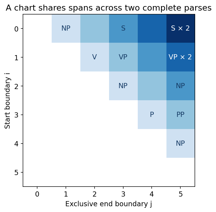
A parser that preserves two analyses
When the grammar permits two attachments, report the alternatives. A parser should not discard ambiguity merely because one option was inserted first. The following standalone parser stores complete small trees in chart cells. This is intentionally simpler than a packed-forest implementation; it suits the five-word demonstration, while the preceding paragraphs explain why explicit enumeration is unsuitable for large ambiguous inputs.
Code · Python · 39 lines
from collections import defaultdict

words = "we saw robots with cameras".split()
lexical = {
    "we": ["NP"], "saw": ["V"], "robots": ["NP"],
    "with": ["P"], "cameras": ["NP"],
}
rules = [
    ("S", "NP", "VP"),
    ("VP", "V", "NP"),
    ("VP", "VP", "PP"),
    ("NP", "NP", "PP"),
    ("PP", "P", "NP"),
]
chart = defaultdict(lambda: defaultdict(list))
for i, word in enumerate(words):
    for category in lexical.get(word, []):
        chart[i, i + 1][category].append((category, word))
for length in range(2, len(words) + 1):
    for start in range(len(words) - length + 1):
        end = start + length
        for split in range(start + 1, end):
            for parent, left, right in rules:
                for left_tree in chart[start, split].get(left, []):
                    for right_tree in chart[split, end].get(right, []):
                        tree = (parent, left_tree, right_tree)
                        if tree not in chart[start, end][parent]:
                            chart[start, end][parent].append(tree)

def bracket(tree):
    if len(tree) == 2:
        return f"({tree[0]} {tree[1]})"
    return f"({tree[0]} {bracket(tree[1])} {bracket(tree[2])})"

parses = chart[0, len(words)].get("S", [])
assert len(parses) == 2
for tree in parses:
    print(bracket(tree))
print("complete parses:", len(parses))
Output
(S (NP we) (VP (V saw) (NP (NP robots) (PP (P with) (NP cameras)))))
(S (NP we) (VP (VP (V saw) (NP robots)) (PP (P with) (NP cameras))))
complete parses: 2
In one tree, the prepositional phrase belongs inside the object noun phrase. In the other, it modifies the verb phrase. Both use every word in order and satisfy the grammar. Choosing between them may require the surrounding scene, prior discourse or lexical preferences beyond these rules.
Add an unknown word and the chart may become empty at a lexical cell. The correct response is a coverage diagnosis. A production service might use a fallback tagger, allow an explicit unknown category or ask for clarification, but each fallback changes the recognized language. It should be documented and tested.
Probabilities over structures
Plain version. A grammar says which analyses exist. A probability model can prefer some analyses and summarize uncertainty across them.
A probabilistic context-free grammar (PCFG) assigns a probability to each production, normalized among rules with the same parent [40]. A derivation has:
Here is a complete derivation tree, indexes each production occurrence in that tree, is its production probability, is the set of permitted parses whose terminal yield is the input , and is the highest-probability parse. The product includes repeated uses of a rule separately.
Replacing chart alternatives with sums computes total probability mass over derivations (the inside algorithm). Replacing them with maxima computes the best derivation (probabilistic CKY). These answer different questions: a sentence with many moderately probable parses can have greater total probability than a sentence with one strong parse, and the best tree need not explain most of the posterior mass. The following snippet computes both for the same five words.
Code · Python · 46 lines
import math
from collections import defaultdict

words = "we saw robots with cameras".split()
lexical = {"we": "NP", "saw": "V", "robots": "NP", "with": "P", "cameras": "NP"}

def parse(p_np_pp):
    # All productions sharing a parent must sum to one, including lexical rules.
    assert 0 < p_np_pp < 1
    rules = {("S", "NP", "VP"): 1.0, ("PP", "P", "NP"): 1.0,
             ("VP", "V", "NP"): 0.6, ("VP", "VP", "PP"): 0.4,
             ("NP", "NP", "PP"): p_np_pp}
    lexical_prob = {"we": (1 - p_np_pp) / 3, "robots": (1 - p_np_pp) / 3,
                    "cameras": (1 - p_np_pp) / 3, "saw": 1.0, "with": 1.0}
    parent_mass = defaultdict(float)
    for (parent, _, _), probability in rules.items():
        parent_mass[parent] += probability
    for word, parent in lexical.items():
        parent_mass[parent] += lexical_prob[word]
    assert all(math.isclose(total, 1.0) for total in parent_mass.values())
    best = defaultdict(dict)    # (i, j) -> {category: (log prob, tree)}
    inside = defaultdict(lambda: defaultdict(float))
    for i, w in enumerate(words):
        best[i, i + 1][lexical[w]] = (math.log(lexical_prob[w]), f"({lexical[w]} {w})")
        inside[i, i + 1][lexical[w]] = lexical_prob[w]
    n = len(words)
    for length in range(2, n + 1):
        for i in range(n - length + 1):
            j = i + length
            for k in range(i + 1, j):
                for (a, b, c), p in rules.items():
                    if b in best[i, k] and c in best[k, j]:
                        score = math.log(p) + best[i, k][b][0] + best[k, j][c][0]
                        if score > best[i, j].get(a, (-math.inf,))[0]:
                            best[i, j][a] = (score, f"({a} {best[i, k][b][1]} {best[k, j][c][1]})")
                        inside[i, j][a] += p * inside[i, k][b] * inside[k, j][c]
    score, tree = best[0, n]["S"]
    return tree, math.exp(score), inside[0, n]["S"]

for p in (0.2, 0.5):
    tree, p_best, p_total = parse(p)
    print(f"P(NP -> NP PP) = {p}: best = {p_best:.6f}, total = {p_total:.6f}")
    print("  ", tree)
    common = ((1 - p) / 3) ** 3
    assert math.isclose(p_total, common * (0.24 + 0.6 * p))
    assert math.isclose(p_best / p_total, max(0.24, 0.6 * p) / (0.24 + 0.6 * p))
Output
P(NP -> NP PP) = 0.2: best = 0.004551, total = 0.006827
   (S (NP we) (VP (VP (V saw) (NP robots)) (PP (P with) (NP cameras))))
P(NP -> NP PP) = 0.5: best = 0.001389, total = 0.002500
   (S (NP we) (VP (V saw) (NP (NP robots) (PP (P with) (NP cameras)))))
The three lexical NP rules share the mass left after the recursive rule: each has probability , where . Both trees contain these three lexical choices, so their common factor is . The verb attachment has probability ; the noun attachment has . Omitting preserves which tree wins within one grammar, but the resulting sum is no longer the probability of the sentence. The code retains it and checks normalization for every parent.
The preferred tree still flips when crosses . Divide a tree’s joint probability by the inside total to obtain its posterior probability given these words. Thus best-tree probability, sentence probability and posterior confidence are three different quantities. The attachment preference here comes from category-rule probabilities rather than lexical context; the next section’s neural scorers add that missing evidence.
Rule probabilities estimated from a treebank depend on the annotation convention and domain. A news-style treebank and a support-message corpus can have different fragment patterns and attachment preferences. Probabilistic modeling supplies a preference mechanism, but it does not remove domain dependence.
Neural constituency parsing: score spans, decode with a chart
Plain version. Instead of multiplying rule probabilities, let a neural encoder score every span and label, then use the same chart to find the highest-scoring tree.
A span-based parser assigns each candidate constituent a score and searches for the tree with the largest total:
Here is a tree viewed as a set of labeled spans with label over the half-open span , is a score computed from contextual vectors at the span boundaries, and is the decoded tree. Stern, Andreas and Klein showed that independent scoring of labels and spans is compatible with classical chart dynamic programming and also admits a greedy top-down decoder that recursively splits the input [5]. Kitaev and Klein replaced the LSTM encoder in that design with self-attention, found that separating positional and content information improved accuracy, and reported 93.55 F1 on the Penn Treebank without external data and 95.13 F1 with pretrained word representations [6]. A follow-up added multilingual pretraining [7].
The output remains a tree even if its scores come from a large neural network: the chart guarantees well-formedness, and the encoder supplies lexical evidence that a PCFG’s rule probabilities could not.
Dependency structure and grammatical roles
Plain version. Dependency analysis links words directly. It highlights which word depends on which other word and labels their grammatical relationship.
A basic dependency tree can be represented by head indices:
Here is the head index of word , denotes an artificial root, is sentence length, is the relation label for that word and is the relation inventory. A valid basic tree additionally requires a specified root convention, connectivity and absence of directed cycles.
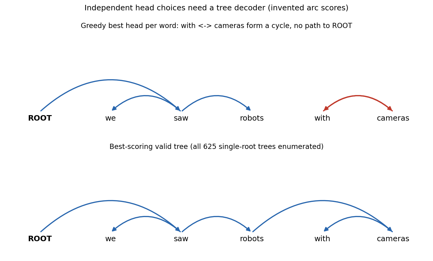
Independent head choices can violate those global requirements. Two words might select each other, forming a cycle. Several disconnected components might attach without a unique sentence root. A tree decoder must enforce the intended structure, or the service must validate and reject an invalid analysis.
Universal Dependencies provides a cross-linguistic annotation framework for morphology, part of speech and grammatical dependencies [8]. Its categories aim for useful comparability across languages while retaining language-specific distinctions. This is an annotation framework, not a claim that every language has identical word order or overt grammatical markers.
Phrase structure and dependencies emphasize different information. A constituent tree makes span grouping explicit. A dependency tree makes lexical heads and relations explicit. Converting between them requires conventions for heads, punctuation and function words; the conversion is not merely a drawing change.
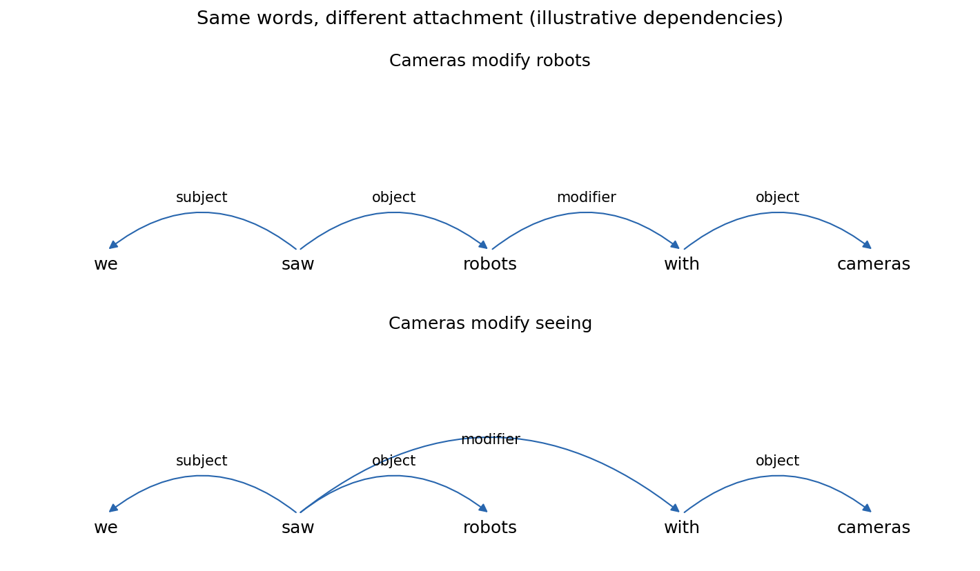
For extraction, grammatical roles are useful evidence but not interchangeable with semantic roles. A passive sentence changes grammatical subject placement while preserving who acted on whom. The semantic-role section below develops that distinction and explains why a dependency arrow does not by itself establish a real-world relation.
Attachment ambiguity reveals a model’s inductive bias
The two camera attachments share their words but assign different participants to the seeing event. Noun-phrase attachment describes a property of the robots. Verb-phrase attachment describes an instrument or circumstance of seeing. A downstream extractor that commits to the noun interpretation might create a robot–camera possession record that the instrument interpretation does not support. An attachment difference is consequential because of the relation it changes, not simply because the brackets look different.
A grammar can permit both while a probability model prefers one, as the PCFG snippet showed. With only parent-category rule probabilities, the model cannot condition that preference on the lexical identity of saw, robots and cameras unless its state or scoring representation is extended. This is a capacity limitation. A wider search over the same score cannot create missing lexical evidence.
The opposite failure is a search limitation: useful scores may exist, but pruning removes the correct span before a complete tree is formed. Diagnose these separately by asking whether the reference structure is representable, whether it survives candidate construction, and whether it receives the highest score among survivors. Each answer suggests a different intervention: extend the representation, revise pruning, or improve scoring.
There is also a genuine information limitation: in an isolated sentence both readings may remain possible, and a gold tree records only the corpus’s chosen interpretation. For an extractor, retaining both alternatives until the required relation is checked can be preferable to an early commitment.
Transition-based dependency parsing
Plain version. Read the sentence left to right with a stack, and at each step choose one of a few actions: shift the next word onto the stack, or attach the top two stack items to each other. A classifier picks the action; the sequence of actions builds the tree.
Nivre formalizes deterministic dependency parsers as transition systems and analyzes stack-based variants (arc-standard and arc-eager, restricted to projective trees) and list-based variants, one of which handles non-projective trees [9]. A projective tree is one whose arcs can be drawn above the sentence without crossing. In the arc-standard system used by Chen and Manning, a configuration has a stack , a buffer and an arc set , and three transitions are available [10]:
Here is the top of the stack and the item below it, is the first buffer word, means stack with on top, is an arc from head to dependent with label , and reads “becomes.” Parsing starts with only the root on the stack and all words in the buffer, and ends when the buffer is empty and only the root remains. Each word is shifted once and reduced once, so a sentence of words needs exactly transitions.
To train the classifier, convert each gold tree into the transition sequence that produces it — a static oracle. The rule below is one standard choice: attach left when the second stack item’s gold head is the top; attach right when the top’s gold head is the second item and the top has already collected all of its own dependents; otherwise shift.
Code · Python · 23 lines
words = ["ROOT", "we", "saw", "robots", "with", "cameras"]
# Gold heads for the instrument reading: "with cameras" attaches to "saw".
gold = {1: 2, 2: 0, 3: 2, 4: 5, 5: 2}

def oracle(gold):
    stack, buffer, arcs, steps = [0], list(range(1, len(words))), {}, []
    def done(h):  # has h already collected all of its dependents?
        return all(d in arcs for d, head in gold.items() if head == h)
    while buffer or len(stack) > 1:
        if len(stack) >= 2 and gold.get(stack[-2]) == stack[-1]:
            dependent = stack.pop(-2)
            arcs[dependent] = stack[-1]; steps.append("LEFT-ARC")
        elif len(stack) >= 2 and gold[stack[-1]] == stack[-2] and done(stack[-1]):
            dependent = stack.pop()
            arcs[dependent] = stack[-1]; steps.append("RIGHT-ARC")
        else:
            stack.append(buffer.pop(0)); steps.append("SHIFT")
    return steps, arcs

steps, arcs = oracle(gold)
print(" ".join(steps))
print({words[d]: words[h] for d, h in sorted(arcs.items())})
assert arcs == gold and len(steps) == 2 * (len(words) - 1)
Output
SHIFT SHIFT LEFT-ARC SHIFT RIGHT-ARC SHIFT SHIFT LEFT-ARC RIGHT-ARC RIGHT-ARC
{'we': 'saw', 'saw': 'ROOT', 'robots': 'saw', 'with': 'cameras', 'cameras': 'saw'}
Ten transitions for five words, as predicted. The done check matters: if robots were attached to saw and popped before cameras arrived, a noun-attachment tree could never be built afterwards. The order of reductions encodes the tree.
At parse time a classifier replaces the oracle. Chen and Manning fed embeddings of words, part-of-speech tags and arc labels from fixed stack and buffer positions into a one-hidden-layer network with a cube activation and a softmax over transitions; their greedy parser is fast but, as they note, exposed to error propagation because an early wrong action cannot be undone [10]. Kiperwasser and Goldberg instead computed one bidirectional-LSTM vector per token, trained jointly with the parser, and built features by concatenating a few of them; the same representation worked for a greedy transition parser and a globally optimized graph parser [12]. Transition parsers run in time linear in sentence length; the price is a local, left-to-right decision procedure.
Graph-based dependency parsing
Plain version. Score every possible head–dependent arc at once, then choose the highest-scoring set of arcs that forms a tree.
McDonald et al. formalize weighted dependency parsing as finding a maximum spanning tree in a directed graph whose nodes are the words plus a root [11]:
Here assigns a head to each word, is the set of head assignments that form a valid tree for sentence , and is the score of the arc from head to dependent . Over projective trees, Eisner’s algorithm solves this in time; over all trees, including non-projective ones, the Chu–Liu–Edmonds maximum-spanning-tree algorithm solves it in [11].
Dozat and Manning made the arc scorer biaffine on top of a deep bidirectional encoder [13]:
Here and are lower-dimensional projections of the contextual vectors of the dependent and the candidate head, is a learned matrix scoring their interaction, and is a learned vector giving each word a prior tendency to be a head. A second biaffine classifier predicts the relation label for the chosen arc. The scorer produces a full matrix of arc scores in one pass.
What does the tree constraint buy? The snippet below uses invented scores for our sentence, picks each word’s best head independently, and then enumerates every single-root tree — feasible only for tiny inputs, but it makes the decoder’s job visible. It finishes with UAS and LAS, defined in the next section.
Code · Python · 39 lines
import itertools
import numpy as np

words = ["ROOT", "we", "saw", "robots", "with", "cameras"]
n = len(words) - 1
# score[h, d]: invented arc scores (head h -> dependent d), not a trained model.
score = np.full((n + 1, n + 1), -2.0)
score[0, 2], score[2, 1], score[2, 3], score[5, 4] = 3.0, 2.0, 2.0, 2.0
score[3, 5], score[2, 5] = 1.5, 1.2                # robots vs saw for "cameras"
score[4, 5] = 1.8                                  # tempting but creates a cycle
np.fill_diagonal(score, -np.inf)

def is_tree(heads):                                # heads[d-1] is the head of d
    if sum(h == 0 for h in heads) != 1:
        return False
    for d in range(1, n + 1):
        seen, node = set(), d
        while node != 0:
            if node in seen:
                return False
            seen.add(node); node = heads[node - 1]
    return True

greedy = [int(np.argmax(score[:, d])) for d in range(1, n + 1)]
total = lambda hs: sum(score[h, d] for d, h in enumerate(hs, start=1))
trees = [hs for hs in itertools.product(range(n + 1), repeat=n)
         if all(h != d for d, h in enumerate(hs, 1)) and is_tree(hs)]
best = max(trees, key=total)
print("greedy heads:", greedy, "valid tree:", is_tree(greedy))
print("best tree:   ", list(best), "score:", round(total(best), 2))
print("trees enumerated:", len(trees))

gold = [2, 0, 2, 5, 2]
labels_gold = ["nsubj", "root", "obj", "case", "obl"]
labels_pred = ["nsubj", "root", "obj", "mark", "nmod"]
uas = np.mean([p == g for p, g in zip(best, gold)])
las = np.mean([p == g and lp == lg for p, g, lp, lg
               in zip(best, gold, labels_pred, labels_gold)])
print(f"UAS = {uas:.2f}, LAS = {las:.2f}")
Output
greedy heads: [2, 0, 2, 5, 4] valid tree: False
best tree:    [2, 0, 2, 5, 3] score: 10.5
trees enumerated: 625
UAS = 0.80, LAS = 0.60
Greedy selection makes with and cameras heads of each other, a two-word cycle disconnected from the root (Figure 3). Among the 625 single-root trees over five words, the best one breaks the cycle and attaches cameras to robots — a valid tree, but the noun reading, while the gold annotation chose the instrument reading. A maximum-spanning-tree algorithm finds the same answer without enumeration.
Graph-based and transition-based parsers make different trade-offs: global search over arc scores with quadratic or cubic decoding, versus linear-time local decisions. Kiperwasser and Goldberg’s shared BiLSTM features served both families [12]. Whichever family is used, the structural guarantee comes from the decoder or transition system, not from the encoder.
Evaluating parsers: PARSEVAL, UAS and LAS
Plain version. Compare the representation that the parser promises to produce, and inspect mistakes where tokenization, annotation or context changes the answer.
The original PARSEVAL procedure compared a candidate parse with a treebank parse after removing material such as punctuation, and computed a crossing-brackets score — how often the candidate brackets a span in a way that crosses a reference bracket — and recall, the number of shared bracket pairs divided by the number in the reference [3]. Today’s standard is labeled bracket precision, recall and F1 [2]:
Here is the set of labeled constituents of tree , is the predicted tree, is the reference tree, and F1 is the harmonic mean of the two. For our two parses, the trees share every labeled bracket except one: the noun-attachment tree has , the verb-attachment tree has . Counting preterminals, each tree has nine labeled constituents, so either tree scored against the other gets precision and recall . State whether lexical preterminals, punctuation and the root are included; different inclusion rules change the denominator.
For dependencies, the unlabeled attachment score (UAS) is the fraction of words with the correct head, and the labeled attachment score (LAS) additionally requires the correct relation:
Here is labeled attachment score, is the set of evaluated word positions, is its size, and are predicted head and relation, and are reference head and relation, and is the indicator function; UAS drops the relation condition. In the snippet, cameras has the wrong head (both scores lose it) and with has the right head with the wrong label (only LAS loses it), giving and .
Token alignment must be fixed before applying these formulas. The CoNLL 2018 shared task asked systems to parse raw text into Universal Dependencies for many languages, without gold-standard annotation on the test input [14]. Systems therefore segment and tokenize for themselves, and predicted words must be aligned with gold words before attachment scores mean anything. If the gold annotation has two words where the tokenizer emits one, an attachment comparison cannot be interpreted normally. Report the segmentation mismatch and specify how alignment is handled. Do not silently delete difficult examples.
Build small diagnostic pairs. Move a modifier while keeping vocabulary similar; add a nested clause; replace an active construction with a passive one; include a fragment or a code-switched phrase. These tests reveal the conditions under which a model’s structure changes, even when an aggregate score appears stable. Avoid treating one gold tree as certainty when the sentence is genuinely ambiguous. A corpus needs a chosen convention or adjudicated analysis, but another analysis may be linguistically reasonable. For an application, ask whether the disagreement changes the extracted fact or action. That connects a parsing error to its practical consequence.
Semantic role labeling: who did what to whom
Plain version. The same event can be expressed with different grammar. Extract the roles in the event instead of assuming the first name is always the actor.
For a simple two-participant predicate, write:
Here names the relation; the first argument is the repairer; and the second argument is the repaired object. “Mina repaired the sensor” and “The sensor was repaired by Mina” can share this representation. Their surface subjects differ. Grammar supplies clues, but a role interpretation must also account for the predicate and construction [1].
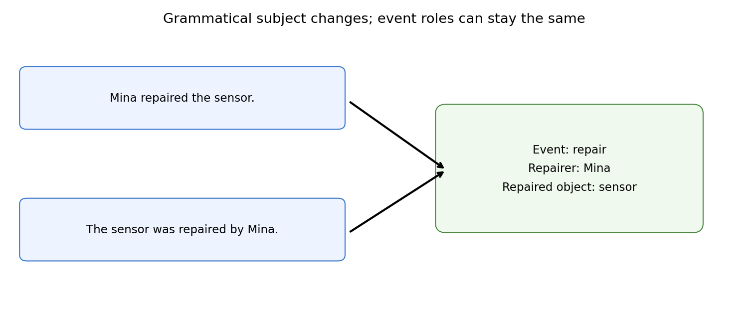
Not every verb permits every alternation, and not every argument is overt. “The sensor was repaired” leaves the repairer unspecified. A system that fills in the nearest previously mentioned person has made a contextual inference, not a direct extraction. That inference may be reasonable, but it needs a separate confidence policy and evidence contract. Preserve an explicit unknown role when the application does not authorize that inference.
Arguments and modifiers also differ. In “Mina repaired the sensor in Taipei on Tuesday,” the repairer and repaired object participate in the core event; location and time modify it. An event schema may include all four fields, but it should say whether each is required. Optional fields prevent an extractor from inventing details merely to satisfy an overly strict schema.
PropBank roles and the SRL task
Gildea and Jurafsky framed automatic semantic role labeling as a statistical task over parsed sentences: match role-bearing phrases to parse constituents, extract features from the words and the tree, and estimate a probability for each possible role [15]. PropBank then annotated the verbs of the Penn Treebank with predicate-specific numbered arguments: each verb sense has a frameset in which Arg0 is typically the agent-like participant and Arg1 the patient or theme, while higher numbers are defined per verb; adjuncts receive ArgM labels such as ArgM-NEG for negation and ArgM-MOD for modals [16]. The numbering is the point: in “an amendment offered by Rep. X,” the amendment is still Arg1 of offer although it is the grammatical subject [16]. The CoNLL-2005 shared task standardized SRL evaluation on PropBank: a predicted argument counts as correct only if its span and role both match, and systems are compared by precision, recall and F1 over arguments [17].
Semantic roles provide a bridge across constructions, not a guarantee of universal agreement. Different resources can label the same participant with predicate-specific or more general roles. Before combining training corpora, compare their definitions and examples. A mechanical label rename can conceal differences about instruments, causes, beneficiaries and implicit participants.
SRL as predicate-conditioned tagging
He et al. cast SRL as BIO sequence tagging, once per predicate: the input marks which word is the predicate, and a deep highway BiLSTM with constrained decoding — forbidding, for example, an I- tag without a preceding B- — labels argument spans [18]. Their eight-layer ensemble reported 83.2 F1 on the CoNLL-2005 test set and found that deep models recover long-distance dependencies but still make surprisingly obvious errors, leaving room for syntactic information to help [18]. With a pretrained encoder, the same design becomes the token-labeling head from NLP 11 plus a predicate indicator. The snippet converts role spans to tag sequences and back, and rejects an invalid sequence.
Code · Python · 34 lines
tokens = "Mina said the sensor was repaired by Lena".split()
# One frame per predicate: (start, end) token spans, end exclusive.
frames = {
    "said":     {"ARG0": (0, 1), "ARG1": (2, 8)},
    "repaired": {"ARG1": (2, 4), "ARG0": (6, 8)},
}

def to_bio(frame, n):
    tags = ["O"] * n
    for role, (i, j) in frame.items():
        tags[i] = "B-" + role
        tags[i + 1:j] = ["I-" + role] * (j - i - 1)
    return tags

def from_bio(tags):
    spans, start, role = {}, None, None
    for k, tag in enumerate(tags + ["O"]):
        if start is not None and not tag.startswith("I-" + role):
            spans[role] = (start, k); start = None
        if tag.startswith("B-"):
            start, role = k, tag[2:]
        elif tag.startswith("I-") and start is None:
            raise ValueError(f"I- tag without B- at position {k}")
    return spans

for predicate, frame in frames.items():
    tags = to_bio(frame, len(tokens))
    tags[tokens.index(predicate)] = "B-V"
    print(f"{predicate:9s}", " ".join(tags))
    assert {r: s for r, s in from_bio(tags).items() if r != "V"} == frame
try:
    from_bio(["O", "I-ARG1", "I-ARG1"])
except ValueError as error:
    print("invalid:", error)
Output
said      B-ARG0 B-V B-ARG1 I-ARG1 I-ARG1 I-ARG1 I-ARG1 I-ARG1
repaired  O O B-ARG1 I-ARG1 O B-V B-ARG0 I-ARG0
invalid: I- tag without B- at position 1
The same sentence yields two frames. For said, Mina is the speaker and the whole reported clause is ARG1. For repaired, Lena is the repairer and the sensor is ARG1 although it is the grammatical subject. An extractor that reads only the repaired frame would record a completed repair as fact; the said frame shows that the repair is Mina’s report. That is exactly the attribution distinction the relation records below must keep.
Scope in semantic representations
Plain version. Small words such as “every,” “some” and “not” can change a statement more than the names do. A semantic parser must record what they modify, or its output answers the wrong question.
NLP 02 introduces quantifier scope and negation with a worked countermodel. Here we look at what scope means for a task output. “Every technician checked a sensor” has a reading in which each technician may check a different sensor and a reading in which one sensor was checked by all. “Mina did not check every sensor” has the form
Here ranges over entities, means sensor, means Mina checked that entity, identifies Mina, means negation and means logical equivalence. A counterexample sensor suffices to make the universal false. “Mina checked no sensor” instead rules out every successful check. Negation’s position determines which evidence can refute the statement.
A document database usually lacks complete knowledge: no extracted inspection record may mean unreported, not false. This difference matters when answering a universal question. A list of observed inspections can support “these sensors were checked,” while establishing “every sensor was checked” also requires the full relevant sensor inventory and complete coverage. Conversely, finding one explicitly unchecked sensor is enough to refute completeness. Scope reasoning and evidence completeness must be considered together. Likewise, “No evidence of failure was found” describes an observation or search result; it should not automatically become “failure is impossible.”
In a restricted extractor, unsupported scope constructions should trigger abstention or review. A rule that handles “did not repair” can still misread “did not say that Mina repaired”: the system must determine what is negated, which is exactly what PropBank’s ArgM-NEG attaches to a specific predicate [16].
Composition is a calculation over roles and scope
A useful way to understand composition is to ask what remains incomplete at each phrase. Mina identifies a participant. repaired requires participants in specified roles. repaired a sensor fixes the object requirement through an existential condition and leaves the actor to be supplied. Combining the subject then closes that requirement. This order of combination explains why identifying the same three content words is insufficient: their roles must be bound correctly [1].
A restricted logical reading of “Mina repaired a sensor” is:
Here ranges over possible entities, means that is a sensor, means that participant repaired , and identifies Mina. The existential quantifier states that at least one suitable entity exists; it does not identify which sensor or imply that every sensor was repaired. This simple reading omits tense and event time intentionally. Those are additional semantic fields, not hidden facts supplied by the notation.
“Only Mina repaired the sensor” adds a restriction on alternatives. “Mina tried to repair the sensor” describes an attempt without guaranteeing a completed repair. “Mina stopped repairing the sensor” changes the event’s temporal interpretation. A record containing only actor and object cannot express those distinctions. This gives a concrete criterion for choosing a representation: list the questions that must be answered, then check whether two source statements requiring different answers collapse into the same record. If both an attempted repair and a completed repair become repair(Mina, sensor), the schema is too coarse for a completion query. A richer encoder cannot prevent that loss after serialization.
Relations, events and provenance
Plain version. A relation links entities; an event organizes participants around an occurrence. Both need evidence, and both can be wrong even when every entity span is right.
A binary relation record can be written:
Here is the record; is the relation type; is the head entity or mention; is the tail entity or mention; and identifies supporting evidence. The letters head and tail define an ordering convention, not a linguistic claim. For an employment relation, reversing the employee and employer changes the record. Define direction in the schema and evaluate it.
Event extraction adds a trigger or event type with multiple roles, such as buyer, seller, item, amount and time — semantic role labeling restricted to an application’s schema. A transaction sentence may mention several prices, only one of which is the actual amount paid. Jointly selecting role assignments can prevent some contradictions, but it cannot resolve an ambiguous source without additional context. Preserve alternatives or route ambiguity to review when the application permits it.
Provenance should include document identity, source version and supporting span. Without a version, offsets can point into a later edited document; without attribution — the said frame above — a quoted allegation becomes an asserted fact. These are properties of the record pipeline, not failures that a larger encoder automatically fixes.
Decompose evaluation by stage — mention detection, category prediction, relation selection and the final supported record — and evaluate relations against predicted mentions as well as gold mentions: perfect input mentions during evaluation can conceal the failure rate of the deployed pipeline.
Discourse, mentions and coreference
Plain version. Meaning continues across sentences. Coreference resolution decides which mentions refer to the same entity, so that facts about “the pump” and “it” end up on the same record.
Discourse is language organized across clauses or sentences. Consider “The pump warmed. The operator stopped it.” The two sentences introduce an event, an agent and a reference to an object. They may suggest a response to warming, but they do not necessarily prove that warming caused the stop. Compare “The pump stopped because the valve closed,” “The pump stopped after the valve closed,” and “The pump stopped although the valve remained open.” The first presents a causal explanation, the second orders events without establishing causation, and the third marks a contrast with an expectation [1]. A summarizer or extractor that inserts “because” has added a claim. Relations also have scope: in “Mina said the pump stopped because the valve closed,” the explanation may be part of Mina’s reported account rather than an independently established finding.
A mention is a text span that refers to an entity, event or concept. An antecedent is an earlier expression that helps interpret another mention. Coreference groups mentions that refer to the same entity. Similar wording does not necessarily imply identity: two different pumps may both be called “the backup pump.”
An antecedent-ranking model
A span-based coreference model can score possible antecedents for a mention, as illustrated by Lee et al. [19]. Abstractly,
Here is the document or conversation; indexes the current mention; is the set of candidate antecedents, including a null option; is the selected antecedent variable; and is a learned compatibility score. The null option permits a mention to introduce a new entity or remain unlinked. Candidate pruning changes what the model can consider. Lee et al.’s model separates the contributions [19]:
Here is the current candidate span, is an earlier candidate span, is the null antecedent, scores whether a span is a mention, and scores pair compatibility. Fixing the null score to zero gives the real links a common reference. Mention pruning saves pairwise computation but can remove the only valid antecedent before linking begins.
The model must detect mentions as well as link them. If an earlier entity span was discarded, a later linking decision cannot recover it merely by assigning better scores among remaining candidates. Separate detection recall from linking accuracy when diagnosing failures.
Clusters complicate supervision. If Pump A, the pump and it refer to one entity, the final mention can correctly link to either earlier mention. A loss that arbitrarily rewards only the nearest one penalizes another valid link. A cluster-based training target instead rewards their combined probability:
Here is the loss for candidate span , is its nonempty set of valid retained antecedents under the annotation and pruning policy, is the antecedent variable, is the document, and is its conditional antecedent probability. The null option belongs in when the span has no valid earlier antecedent. This is marginalization over valid links, as used in the original model [19]. At inference, connecting mentions through antecedent links forms entity groups. A single erroneous bridge can merge two otherwise coherent groups, and the wrongly merged cluster can later assign several events to the wrong pump.
A recency baseline and its failure
The following hand-written baseline uses explicit compatibility and recency. It is deliberately small enough to expose a failure. Device categories are supplied as data; the code does not infer attributes from personal names or social stereotypes.
Code · Python · 19 lines
entities = [
    {"id": "pump_a", "category": "device", "turn": 1},
    {"id": "valve_b", "category": "device", "turn": 2},
    {"id": "operator", "category": "person", "turn": 2},
]
def candidates(category):
    return [e for e in entities if e["category"] == category]
def recent(category):
    choices = candidates(category)
    return max(choices, key=lambda e: e["turn"])["id"] if choices else None
print("Recency baseline for it:", recent("device"))
assert recent("device") == "valve_b"
# In a synthetic annotation, the speaker meant the earlier pump.
intended = "pump_a"
assert recent("device") != intended
# A cautious application preserves ambiguity instead of hiding the choice.
possible = {e["id"] for e in candidates("device")}
resolution = next(iter(possible)) if len(possible) == 1 else None
assert resolution is None and possible == {"pump_a", "valve_b"}
The baseline prints valve_b, while the constructed speaker intention points to the earlier pump. A cue cannot establish identity in every case. A clarifying question such as “Do you mean Pump A or Valve B?” preserves the uncertainty explicitly; NLP 08 develops clarification in dialogue.
Context can include deixis: “this,” “here” or “now” depend on a speaker, place, time or interface selection, so store that context with the utterance, and do not score a system as wrong for refusing an inference the input cannot support. Quotation adds constraints too: I in an operator’s quoted statement refers to that operator, and “the other pump” presupposes a contrast set that a recency rule does not define.
Optional: End-to-end coreference (in the Paper guides). Follow the original figure, objective, experimental comparisons and limitations.
Evaluating coreference: MUC, B³, CEAF and CoNLL F1
Plain version. A coreference output is a partition of mentions into entities. Different metrics count agreement between two partitions in different units — links, mentions or entities — so no single one tells the whole story.
Let be the key (gold) partition and the response partition.
- MUC is link-based [20]. For each key entity , let be the partition of induced by the response, with unmatched mentions as singletons. Recall is : the number of key links the response preserves over the minimum number of links needed. Precision swaps the roles of key and response.
- B³ is mention-based. For each mention , compare the key entity and response entity containing it: recall averages and precision averages over mentions [23].
- CEAF is entity-based [21]. It finds the best one-to-one alignment between key and response entities, a maximum bipartite matching. With the entity similarity (the entity-based variant CEAF), recall is the total aligned similarity divided by the number of key entities and precision divides by the number of response entities.
The CoNLL-2012 shared task scored systems by the unweighted mean of MUC, B³ and CEAF F1, on the grounds that each represents a different dimension [23]. Pradhan et al. later published a reference scorer because inconsistent implementations, especially for predicted mentions that do not match gold mentions, had produced incomparable numbers [22]. The snippet computes all three for the response in Figure 5, where “it” is wrongly merged with the valve.
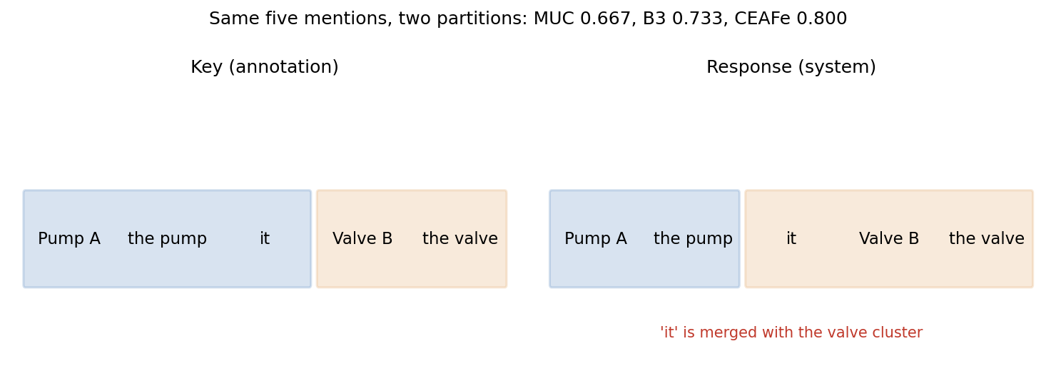
Code · Python · 36 lines
import numpy as np
from scipy.optimize import linear_sum_assignment

# Mentions: a="Pump A", b="the pump", c="it", d="Valve B", e="the valve"
key = [{"a", "b", "c"}, {"d", "e"}]
response = [{"a", "b"}, {"c", "d", "e"}]          # "it" wrongly joined to the valve

def f1(p, r):
    return 2 * p * r / (p + r) if p + r else 0.0

def muc(gold, pred):                                # link-based
    def recall(g, p):
        def parts(s):  # pieces of s cut by p; uncovered mentions are singletons
            covered = set().union(*p)
            return sum(1 for t in p if s & t) + len(s - covered)
        return sum(len(s) - parts(s) for s in g) / sum(len(s) - 1 for s in g)
    return recall(pred, gold), recall(gold, pred)    # precision, recall

def b_cubed(gold, pred):                            # mention-based
    def score(a, b):
        cluster_of = {m: s for s in b for m in s}
        return np.mean([len(s & cluster_of.get(m, set())) / len(s)
                        for s in a for m in s])
    return score(pred, gold), score(gold, pred)

def ceaf_e(gold, pred):                             # entity-based
    phi = np.array([[2 * len(g & p) / (len(g) + len(p)) for p in pred] for g in gold])
    rows, cols = linear_sum_assignment(-phi)
    total = phi[rows, cols].sum()
    return total / len(pred), total / len(gold)

scores = {name: f1(*fn(key, response)) for name, fn in
          [("MUC", muc), ("B3", b_cubed), ("CEAFe", ceaf_e)]}
for name, value in scores.items():
    print(f"{name:6s} F1 = {value:.3f}")
print(f"CoNLL F1 = {np.mean(list(scores.values())):.3f}")
Output
MUC    F1 = 0.667
B3     F1 = 0.733
CEAFe  F1 = 0.800
CoNLL F1 = 0.733
Check MUC by hand: the key needs links; the response splits the pump entity into two pieces and keeps the valve entity whole, preserving links, so recall is , and by symmetry precision is . B³ penalizes each affected mention, and CEAF still aligns each key entity with a mostly-correct response entity. One error, three numbers: that is why the shared task averaged them, and why an application should also check the records that consume the clusters.
Scores are interpretable only relative to the annotation policy: whether events and associative relations are linked, whether singletons count, and how ambiguity is annotated.
Semantic parsing and AMR
Plain version. Semantic parsing maps a sentence to a meaning representation that a program can use: a logical form, a database query or a graph. Abstract Meaning Representation (AMR) is a widely used whole-sentence graph format.
Banarescu et al. designed AMR for “sembanking”: AMRs are rooted, labeled, directed graphs that are easy for people to read and programs to traverse; they aim to abstract away from syntactic idiosyncrasies, assigning the same AMR to sentences with the same basic meaning, and they make extensive use of PropBank framesets [24]. When one entity plays several roles, AMR uses re-entrancy — a node with multiple parents — so the graph is not a tree. In “the operator wants to stop the pump,” the operator is ARG0 of both want-01 and stop-01. AMR deliberately does not specify how the graph is derived from the words, which makes alignment between words and nodes a separate problem [24].
Smatch evaluates AMR parsing by viewing each graph as a conjunction of triples, either instance(variable, concept) or relation(variable1, variable2), and reporting precision, recall and F1 of matched triples under the variable mapping that maximizes the match [25]. Finding that mapping is NP-complete, so the paper provides an integer-linear-programming method and a hill-climbing heuristic with random restarts [25]. For a four-variable graph, we can simply try every mapping:
Code · Python · 20 lines
import itertools

# "the operator wants to stop the pump" vs a parse that loses who stops.
gold = {("instance", "w", "want-01"), ("instance", "o", "operator"),
        ("instance", "s", "stop-01"), ("instance", "p", "pump"),
        ("ARG0", "w", "o"), ("ARG1", "w", "s"),
        ("ARG0", "s", "o"), ("ARG1", "s", "p")}
pred = {("instance", "a", "want-01"), ("instance", "b", "operator"),
        ("instance", "c", "stop-01"), ("instance", "d", "pump"),
        ("ARG0", "a", "b"), ("ARG1", "a", "c"), ("ARG1", "c", "d")}

def rename(triples, mapping):
    return {(r, mapping.get(x, x), mapping.get(y, y)) for r, x, y in triples}

pred_vars, gold_vars = sorted({t[1] for t in pred}), sorted({t[1] for t in gold})
best = max(len(rename(pred, dict(zip(pred_vars, perm))) & gold)
           for perm in itertools.permutations(gold_vars))
precision, recall = best / len(pred), best / len(gold)
print("matched triples:", best)
print(f"Smatch P={precision:.3f} R={recall:.3f} F1={2*precision*recall/(precision+recall):.3f}")
Output
matched triples: 7
Smatch P=1.000 R=0.875 F1=0.933
The predicted graph is missing one triple — the re-entrant ARG0 edge that says the operator is also the one stopping. Smatch still gives 0.933. For a safety application, “who stops the pump” may be the whole question. Like every aggregate metric in this chapter, Smatch should be paired with targeted checks on the relations that matter.
How pretrained models changed these tasks
Plain version. Pretrained encoders turned parsers, role labelers and coreference systems into “encoder plus small structured decoder.” They did not remove the need for the decoder, the annotation scheme or careful evaluation.
Three shifts stand out. First, features were replaced by contextual vectors. Kitaev and Klein’s parser improved from 93.55 to 95.13 F1 when it used pretrained word representations [6]; Joshi et al. applied BERT to coreference and reported a gain of 3.9 F1 over the previous state of the art on OntoNotes, noting remaining weaknesses in document-level context, conversations and mention paraphrasing [26]. SpanBERT changed the pretraining objective itself — masking contiguous spans and training span-boundary representations to predict the span content — and reported 79.6% F1 on OntoNotes coreference along with 94.6 and 88.7 F1 on SQuAD 1.1 and 2.0 [27]. Span-shaped tasks benefited from span-shaped pretraining.
Second, the structures turned out to be partly present inside the encoders. Hewitt and Manning’s structural probe found a linear transformation under which squared distance between word vectors encodes distance in the parse tree, for ELMo and BERT but not for baselines [28]. Tenney, Das and Pavlick found that BERT represents the steps of the traditional pipeline in an interpretable order across layers — part-of-speech tagging, parsing, named entities, semantic roles, then coreference — while sometimes revising lower-level decisions using higher-level information [29]. These are probing results: they show that information is linearly recoverable, not that the model uses it the way a parser does.
Third, the pipeline collapsed into fine-tuning and prompting. Encoders supply evidence for tags and trees, and large language models can be prompted to return structures [30]. An output validator remains necessary: a plausible bracketed string can omit a token, reorder words or fail to form a connected tree.
Modern view
Surveys and their taxonomies. Zhang’s survey of syntactic–semantic parsing focuses on the two most popular formalizations, constituent and dependency parsing, reviews representative models for each and for semantic dependency graphs, and covers cross-domain, cross-lingual and joint parsing as well as corpus development [31]. Poesio et al.’s review of computational models of anaphora traces coreference from pre-neural work through current neural models, surveys the annotated datasets, and treats less-studied phenomena such as bridging reference and discourse deixis [32]. Chen et al.’s SRL survey, accepted at Artificial Intelligence Review, proposes a four-dimensional taxonomy — model architectures, syntax feature modeling, application scenarios and multimodal extensions — analyzes when syntactic features help, and examines the complementary roles of LLMs and specialized SRL systems [34]. Zhao et al.’s LLM survey distinguishes model training, adaptation, utilization and capacity evaluation [30]; structure can play several roles within that taxonomy — a supervised output, an internal representational probe, a constraint on generation or a diagnostic challenge. Chang et al.’s evaluation survey further separates the tasks being measured from the benchmarks and protocols used [33].
Recent original work (2023–2026). Tian, Xia and Song found that LLMs are effective at shallow parsing (chunking) but struggle to produce correct full constituency trees, and improved them by prompting for chunks first and filtering them [35]. Hale and Stanojević tested a candidate syntactic universal across typologically diverse languages and found that the model they studied respected it only in some higher-resource languages [36], illustrating why an English-focused structural test cannot establish uniform multilingual competence. For coreference, Le and Ritter found that prompting instruction-tuned models can outperform unsupervised coreference systems but relies on high-quality mention detection [37]; Porada, Zou and Cheung controlled for the pretrained language model across five coreference systems and found that encoder-based models outperformed more recent decoder-based ones at equal model size, and that controlling for the encoder removes most, but not all, of the reported F1 gains of the preceding five years [38]. For semantic representations, Jin et al. found that feeding AMR into LLM chain-of-thought prompting generally hurt more than it helped across five tasks, with errors concentrated in multi-word expressions, named entities and the final inference step [39].
Distinguish valid structure from structural generalization
These studies motivate two different tests. First, can a system produce a legal structure for this annotation scheme? Second, does its choice respond to the grammatical distinction rather than a familiar word sequence? A structural validator addresses the first and cannot establish the second. A model that always returns one conventional attachment can pass format checks while failing a controlled contrast.
Construct comparisons that hold lexical content nearly fixed while changing the role-relevant construction (active versus passive, modifier relocation, a relative clause), then vary vocabulary while holding the construction fixed. If an unfamiliar noun changes the whole structure, lexical coverage is interfering; if a grammatical change leaves the interpretation untouched, a familiar lexical pattern dominates. Finally check whether mistakes alter the semantic roles needed downstream.
Longer context changes the reference decision, not only memory size
A longer history can restore a missing antecedent, but it also adds compatible candidates; in an antecedent softmax, a new candidate changes the denominator even when existing link scores stay fixed, so thresholds calibrated on short histories need not transfer. Compare a short history, a long irrelevant history and a long history containing another device of the same type to separate useful context from merely more text.
Open problems. Annotation schemes differ; low-resource languages lack enough independently checked trees; segmentation interacts with syntax; spontaneous dialogue contains fragments and repairs; coreference across long documents and conversations remains hard; and a system can learn benchmark-specific conventions without robust compositional behavior. Preserving alternative analyses, testing structural minimal pairs, controlling for the encoder when comparing architectures [38], and measuring downstream consequences offer concrete ways to study those limits.
Key takeaways
- A grammar’s failure to parse is a coverage result, not a judgment of a speaker; charts share spans, but enumerating all trees can still grow exponentially.
- Best-tree (max) and total-probability (sum) answer different questions; rule probabilities alone cannot see lexical evidence, which is what neural span and arc scorers add.
- Transition parsers make linear-time local decisions; graph parsers score all arcs and need a tree decoder, because independent head choices can form cycles.
- Each structure has its own metric — labeled brackets, UAS/LAS, argument F1, MUC/B³/CEAF, Smatch — and each needs a stated denominator and alignment policy.
- Semantic roles survive grammatical alternations; PropBank numbers arguments per predicate and marks negation and modality as adjuncts.
- Preserve scope, attribution and provenance in extracted records; a coarse schema loses distinctions that no encoder can recover afterwards.
- Coreference is detection plus linking; one wrong bridge can merge entities, and an explicit ambiguous outcome is better than a confident wrong one.
- Pretrained encoders improved and simplified these systems, but validity still comes from the decoder and evaluation from the annotation scheme.
Exercises
- A grammar extension. Extend the chart parser to accept “we saw cameras” and a new preposition. Then add an unseen noun and explain which lexical change is required.
Hint
The existing binary rules already support the shorter sentence. Coverage of terminals is a separate issue from phrase combination.
- Recognition versus enumeration. Replace tree lists with Boolean categories in the chart. Compare what the parser can still answer and what information it loses. Then change the PCFG snippet so that the noun attachment wins with the original rule probabilities, by adding a lexicalized rule score for
robots with.
Hint
Acceptance remains available without trees; recovering alternative attachments needs backpointers. For the lexicalized variant, multiply the score by a factor that depends on the head noun.
- A structural validator and a non-projective tree. Write checks for token yield, one head per word, no self-links, a unique root and absence of cycles in a basic dependency tree. Then construct a valid tree for a short sentence whose arcs cross, and explain why the arc-standard oracle cannot produce it.
Hint
Following head pointers from each word should reach the root without visiting a word twice. Arc-standard only attaches the top two stack items, so every arc it creates spans a contiguous, already-completed region.
- Two readings, two records. Write two interpretations of “A technician inspected every sensor.” Design a relation schema that can store either reading, and an evidence rule for answering “Was every sensor inspected?” from a document collection.
Hint
Compare an existential quantifier outside a universal quantifier with the reverse order. The answer requires a sensor inventory and coverage information, not only extracted inspection events.
- Coreference metrics. Construct a response that merges all five mentions of Figure 5 into one entity, and another that leaves all five as singletons. Compute MUC, B³ and CEAF for both before running the code, then explain which metric is most lenient to each mistake.
Hint
MUC counts links, so a single giant cluster preserves every key link. B³ penalizes each mention whose cluster contains wrong members. Singletons have no links at all.
- Bilingual deixis. Write a bilingual message containing a demonstrative, a relative date and an indirect request, for example mixing English and Chinese. Describe two contexts that change its interpretation, and list the evidence a coreference or extraction system would need to distinguish them.
Hint
A forwarded quotation changes whose viewpoint controls “I,” “here” and “tomorrow.” An ability test and a maintenance conversation can give the same question different purposes.
References
- Susan McRoy, Principles of Natural Language Processing, Chapters 3–5 and 7 and the chart-parsing appendix, open textbook, 2021. Open textbook
- Daniel Jurafsky and James H. Martin, Speech and Language Processing, 3rd ed. draft (August 19, 2026), Chapters 19, 20, 22 and 24. Book site
- E. Black, S. Abney, D. Flickenger, C. Gdaniec, R. Grishman, P. Harrison, D. Hindle, R. Ingria, F. Jelinek, J. Klavans, M. Liberman, M. Marcus, S. Roukos, B. Santorini and T. Strzalkowski, “A Procedure for Quantitatively Comparing the Syntactic Coverage of English Grammars,” Speech and Natural Language Workshop, 1991. Paper
- Mitchell P. Marcus, Beatrice Santorini and Mary Ann Marcinkiewicz, “Building a Large Annotated Corpus of English: The Penn Treebank,” Computational Linguistics 19(2), 1993. Paper
- Mitchell Stern, Jacob Andreas and Dan Klein, “A Minimal Span-Based Neural Constituency Parser,” ACL, 2017. Paper
- Nikita Kitaev and Dan Klein, “Constituency Parsing with a Self-Attentive Encoder,” ACL, 2018. Paper
- Nikita Kitaev, Steven Cao and Dan Klein, “Multilingual Constituency Parsing with Self-Attention and Pre-Training,” ACL, 2019. Paper
- Marie-Catherine de Marneffe, Christopher D. Manning, Joakim Nivre and Daniel Zeman, “Universal Dependencies,” Computational Linguistics 47(2), 2021. Paper
- Joakim Nivre, “Algorithms for Deterministic Incremental Dependency Parsing,” Computational Linguistics 34(4), 2008. Paper
- Danqi Chen and Christopher Manning, “A Fast and Accurate Dependency Parser using Neural Networks,” EMNLP, 2014. Paper
- Ryan McDonald, Fernando Pereira, Kiril Ribarov and Jan Hajič, “Non-Projective Dependency Parsing using Spanning Tree Algorithms,” HLT-EMNLP, 2005. Paper
- Eliyahu Kiperwasser and Yoav Goldberg, “Simple and Accurate Dependency Parsing Using Bidirectional LSTM Feature Representations,” Transactions of the ACL 4, 2016. Paper
- Timothy Dozat and Christopher D. Manning, “Deep Biaffine Attention for Neural Dependency Parsing,” ICLR, 2017. Paper
- Daniel Zeman, Jan Hajič, Martin Popel, Martin Potthast, Milan Straka, Filip Ginter, Joakim Nivre and Slav Petrov, “CoNLL 2018 Shared Task: Multilingual Parsing from Raw Text to Universal Dependencies,” CoNLL Shared Task, 2018. Paper
- Daniel Gildea and Daniel Jurafsky, “Automatic Labeling of Semantic Roles,” Computational Linguistics 28(3), 2002. Paper
- Martha Palmer, Daniel Gildea and Paul Kingsbury, “The Proposition Bank: An Annotated Corpus of Semantic Roles,” Computational Linguistics 31(1), 2005. Paper
- Xavier Carreras and Lluís Màrquez, “Introduction to the CoNLL-2005 Shared Task: Semantic Role Labeling,” CoNLL, 2005. Paper
- Luheng He, Kenton Lee, Mike Lewis and Luke Zettlemoyer, “Deep Semantic Role Labeling: What Works and What’s Next,” ACL, 2017. Paper
- Kenton Lee, Luheng He, Mike Lewis and Luke Zettlemoyer, “End-to-end Neural Coreference Resolution,” EMNLP, 2017. Paper
- Marc Vilain, John Burger, John Aberdeen, Dennis Connolly and Lynette Hirschman, “A Model-Theoretic Coreference Scoring Scheme,” MUC-6, 1995. Paper
- Xiaoqiang Luo, “On Coreference Resolution Performance Metrics,” HLT-EMNLP, 2005. Paper
- Sameer Pradhan, Xiaoqiang Luo, Marta Recasens, Eduard Hovy, Vincent Ng and Michael Strube, “Scoring Coreference Partitions of Predicted Mentions: A Reference Implementation,” ACL, 2014. Paper
- Sameer Pradhan, Alessandro Moschitti, Nianwen Xue, Olga Uryupina and Yuchen Zhang, “CoNLL-2012 Shared Task: Modeling Multilingual Unrestricted Coreference in OntoNotes,” EMNLP-CoNLL Shared Task, 2012. Paper
- Laura Banarescu, Claire Bonial, Shu Cai, Madalina Georgescu, Kira Griffitt, Ulf Hermjakob, Kevin Knight, Philipp Koehn, Martha Palmer and Nathan Schneider, “Abstract Meaning Representation for Sembanking,” Linguistic Annotation Workshop, 2013. Paper
- Shu Cai and Kevin Knight, “Smatch: an Evaluation Metric for Semantic Feature Structures,” ACL, 2013. Paper
- Mandar Joshi, Omer Levy, Luke Zettlemoyer and Daniel Weld, “BERT for Coreference Resolution: Baselines and Analysis,” EMNLP-IJCNLP, 2019. Paper
- Mandar Joshi, Danqi Chen, Yinhan Liu, Daniel S. Weld, Luke Zettlemoyer and Omer Levy, “SpanBERT: Improving Pre-training by Representing and Predicting Spans,” Transactions of the ACL 8, 2020. Paper
- John Hewitt and Christopher D. Manning, “A Structural Probe for Finding Syntax in Word Representations,” NAACL-HLT, 2019. Paper
- Ian Tenney, Dipanjan Das and Ellie Pavlick, “BERT Rediscovers the Classical NLP Pipeline,” ACL, 2019. Paper
- Wayne Xin Zhao et al., “A Survey of Large Language Models,” Frontiers of Computer Science, 2026; online manuscript updated March 2026. Survey
- Meishan Zhang, “A survey of syntactic-semantic parsing based on constituent and dependency structures,” Science China Technological Sciences 63, 2020. Survey
- Massimo Poesio, Juntao Yu, Silviu Paun, Abdulrahman Aloraini, Pengcheng Lu, Janosch Haber and Derya Cokal, “Computational Models of Anaphora,” Annual Review of Linguistics 9, 2023. Survey
- Yupeng Chang et al., “A Survey on Evaluation of Large Language Models,” ACM Transactions on Intelligent Systems and Technology, 2024. Survey
- Huiyao Chen, Meishan Zhang, Jing Li, Lilja Øvrelid, Jan Hajič, Hao Fei and Min Zhang, “A Systematic Survey of Semantic Role Labeling in the Era of Pretrained Language Models,” arXiv:2502.08660, 2025; accepted at Artificial Intelligence Review. Survey
- Yuanhe Tian, Fei Xia and Yan Song, “Large Language Models are No Longer Shallow Parsers,” ACL, 2024. Paper
- John T. Hale and Miloš Stanojević, “Do LLMs learn a true syntactic universal?” EMNLP, 2024. Paper
- Nghia T. Le and Alan Ritter, “Are Large Language Models Robust Coreference Resolvers?” arXiv:2305.14489, 2023. Paper
- Ian Porada, Xiyuan Zou and Jackie Chi Kit Cheung, “A Controlled Reevaluation of Coreference Resolution Models,” LREC-COLING, 2024. Paper
- Zhijing Jin, Yuen Chen, Fernando Gonzalez Adauto, Jiarui Liu, Jiayi Zhang, Julian Michael, Bernhard Schölkopf and Mona Diab, “Analyzing the Role of Semantic Representations in the Era of Large Language Models,” NAACL, 2024. Paper
- NLTK contributors,
nltk.grammar.PCFG, API documentation, accessed 2026-11-05. Normalization contract
Check your understanding
This tutorial has 6 exercises. Can you solve them without opening the hints?
Go to the exercises ↑This is the last tutorial in Natural Language Processing. Back to the learning map →