NLP 04 · Lexical Semantics and Word Embeddings
Needs: NLP 03 · Neural Networks for NLP
Navigate: this page and this track: Navigate: this page and this track
On this page
- What you’ll learn1 min
- The big picture2 min
- Lexical semantics: senses and relations2 min
- Distributional evidence: contexts are observations1 min
- Count-based embeddings: inspect the shared-context assumption2 min
- Word2Vec: learn a word by predicting its neighbors8 min
- GloVe: fit log co-occurrence counts directly2 min
- fastText: vectors from character n-grams1 min
- Dense word and document representations3 min
- Evaluating word embeddings3 min
- Bias in embeddings1 min
- From word vectors to sentence embeddings3 min
- Preview: contextual embeddings1 min
- Modern view2 min
- Key takeaways1 min
- Exercises2 min
- Paper guides
- References
Natural Language Processing
Explore this chapter 2 interactive experiments
Pad a three-word sentence with zero vectors and compare a correct masked mean with a mean that counts the padding in its denominator.
What you’ll learn
- Distinguish word forms, lemmas and senses, and name the main lexical relations: synonymy, antonymy, hypernymy and meronymy, as organized in WordNet.
- Explain the distributional hypothesis, what shared contexts can reveal about words and what they cannot establish.
- Construct a word–context matrix, turn positive PMI into compact vectors, and derive CBOW, Skip-gram, negative sampling, GloVe and fastText objectives.
- Evaluate embeddings with similarity and analogy tests while recognizing their caveats, and measure an association bias.
- Pool word vectors into sentence representations, train sentence embeddings contrastively, and explain what changes with contextual embeddings.
The big picture
A word ID identifies a vocabulary entry. Its numerical value says nothing about what the word does in language. An embedding assigns that entry a learned vector, allowing words to share useful statistical patterns. The central question is not simply how to make a vector smaller. It is which evidence and objective should determine its coordinates.
Linguists describe word meaning with lexical semantics: senses, and relations such as synonymy and hypernymy, recorded by hand in resources like WordNet. Distributional methods learn vectors from text instead. This lesson connects the two views. Hagiwara develops word and document embeddings as reusable features for practical applications [1]. McRoy distinguishes lexical similarity from language tasks such as sentiment and entailment [2]. Here we develop the representation itself, and we keep asking which lexical relation a vector geometry actually captures.
NLP 03 learned word vectors as a by-product of a task: an embedding layer inside a classifier, and the table inside the neural probabilistic language model of Bengio et al. [3]. Word2Vec makes the vectors themselves the goal and uses nearby words, not a following word, as the prediction target. These are different prediction contracts:
| Question | Neural probabilistic language model | Static Word2Vec embedding |
|---|---|---|
| What is observed? | An ordered history of tokens and the token that follows | A center word and selected neighbors on both sides |
| What is predicted? | A normalized distribution over the next token | A center from neighbors, or individual neighbors from a center |
| Is left-to-right generation the purpose? | Yes; it is a language model | Basic window training is not an ordered generator |
| What is reused afterward? | The whole network; word vectors are a by-product | A learned vector table |
Continuous in CBOW means that its internal representation has real-valued coordinates. It does not mean that the text is continuous, that words occur without boundaries, or that every word sense receives its own vector. By the end, we will connect the count-based and prediction-based constructions and identify exactly which information each retains. Count-based language models and their evaluation come later, in NLP 05.
Lexical semantics: senses and relations
Plain version. A written word can carry several meanings, and meanings relate to each other in structured ways: some are near-equivalents, some are opposites, some are kinds of others. Embeddings will later blur several of these relations together, so name them first.
Word forms, lemmas and senses
A word form is what appears in text (banks, banked); a lemma is the dictionary entry that groups inflected forms (bank). A sense is one meaning of a lemma. bank has at least two unrelated senses, the slope beside a river and the financial institution; this is homonymy. window has related senses, an opening in a wall and a region of a screen; this is polysemy. NLP 02 discusses how context and composition select a sense. For representation, the key point is that a vocabulary entry is a form or lemma, not a sense: a table with one row per entry must merge every sense of that entry.
Relations between senses
Lexical relations hold between senses, not between spelling strings:
- Synonymy: two senses that can substitute for each other in many contexts with little change in meaning, such as
slopeandincline. Exact synonymy is rare; register, collocation and connotation usually differ. - Antonymy: senses that are opposite along one scale or dimension, such as
hotandcold. Antonyms are otherwise very similar: they describe the same property and occur in the same kinds of sentences. - Hyponymy and hypernymy: an is-a relation.
poodleis a hyponym ofdog, anddogis a hypernym ofpoodle. The relation is asymmetric and usually transitive, forming a hierarchy. - Meronymy: a part–whole relation, such as
wheelandcar.
Two further notions matter for evaluation. Similarity asks whether two concepts share properties (cup and mug); relatedness or association asks whether they tend to occur together (cup and coffee). A related pair need not be similar at all.
WordNet: a hand-built lexical database
WordNet organizes English nouns, verbs, adjectives and adverbs into synsets, sets of synonymous lemmas that express one concept, each with a short gloss, connected by relations such as hypernymy, meronymy and antonymy [4]. Looking up a lemma returns its synsets, one per sense. Walking hypernym links from a synset reaches increasingly general concepts, which lets a program measure how far apart two senses are in the hierarchy.
The following example builds a miniature database in the same style, by hand, to show the mechanics without downloading WordNet itself. Its entries are invented for this lesson.
Code · Python · 31 lines
# A hand-built miniature lexical database in the style of WordNet (not WordNet data).
synsets = {
    "bank.n.slope":   {"lemmas": ["bank"], "gloss": "sloping land beside a river", "hypernym": "slope.n"},
    "bank.n.finance": {"lemmas": ["bank"], "gloss": "an institution that holds deposits", "hypernym": "institution.n"},
    "slope.n":        {"lemmas": ["slope", "incline"], "gloss": "a surface at an angle", "hypernym": "landform.n"},
    "landform.n":     {"lemmas": ["landform"], "gloss": "a natural feature of land", "hypernym": "entity.n"},
    "institution.n":  {"lemmas": ["institution"], "gloss": "an organization with a public role", "hypernym": "organization.n"},
    "school.n":       {"lemmas": ["school"], "gloss": "an institution for teaching", "hypernym": "institution.n"},
    "organization.n": {"lemmas": ["organization"], "gloss": "a group with a purpose", "hypernym": "entity.n"},
    "entity.n":       {"lemmas": ["entity"], "gloss": "anything that exists", "hypernym": None},
}

def senses(word):
    return [s for s, v in synsets.items() if word in v["lemmas"]]

def path_to_root(s):
    path = [s]
    while synsets[path[-1]]["hypernym"]:
        path.append(synsets[path[-1]]["hypernym"])
    return path

def path_similarity(a, b):            # 1 / (1 + edges on the shortest is-a path)
    pa, pb = path_to_root(a), path_to_root(b)
    common = next(s for s in pa if s in pb)
    return 1 / (1 + pa.index(common) + pb.index(common))

print("senses of bank:", senses("bank"))
print("synonyms in slope.n:", synsets["slope.n"]["lemmas"])
print("hypernym chain:", " -> ".join(path_to_root("bank.n.finance")))
for other in ["school.n", "slope.n"]:
    print(f"path_similarity(bank.n.finance, {other}) = {path_similarity('bank.n.finance', other):.3f}")
The run prints:
Code · 5 lines
senses of bank: ['bank.n.slope', 'bank.n.finance']
synonyms in slope.n: ['slope', 'incline']
hypernym chain: bank.n.finance -> institution.n -> organization.n -> entity.n
path_similarity(bank.n.finance, school.n) = 0.333
path_similarity(bank.n.finance, slope.n) = 0.167
The financial sense of bank is closer to school (both are institutions) than to slope, even though the other sense of bank is a kind of slope. A sense inventory makes that distinction explicit; a single vector for the string bank cannot.
Hand-built resources are precise and interpretable, but they are expensive to build, cover some languages and domains far better than others, lag behind new words and senses, and encode one set of sense distinctions that may not match an application. Distributional vectors make the opposite trade: they are cheap and broad, but their relations are implicit and mixed. Much practical work combines the two, for example by checking embedding neighbors against a lexical resource.
Distributional evidence: contexts are observations
Plain version. Words that appear in similar surroundings can acquire similar vectors. The surroundings provide evidence about usage; they do not directly supply definitions or truth conditions.
Harris argued that differences in meaning correlate with differences in distribution: the environments in which linguistic elements occur [5]. This distributional hypothesis is the foundation of every method in the rest of this lesson.
A word type is a vocabulary entry, while a word token is one occurrence. A static embedding pools evidence across many tokens into one vector for the type. Occurrences of bank beside river and beside account therefore influence the same row. The model can learn that the word has mixed usage, but the lookup operation cannot choose a different row for each sense.
Define context before collecting statistics. A radius-two word window contains up to two tokens on each side of the center, excluding the center itself. A shorter window emphasizes immediate surroundings; a larger one includes more distant topic evidence. If direction matters, left and right context positions can be separate features. Our examples deliberately merge the two sides so the model’s invariance is visible.
The distributional assumption is useful because text provides repeated observations without requiring a semantic label for every word. It is incomplete because shared use includes synonymy, opposition, thematic association and grammatical compatibility. hot and cold can both appear before water; similarity on that evidence does not establish that they express the same property. In the terms of the previous section, distributional similarity mixes synonymy, antonymy, co-hyponymy and relatedness. Turney and Pantel organize these vector-space approaches by the evidence represented in their matrices [6].
Keep corpus, tokenizer and window specification together. Changing word segmentation changes the types whose contexts are counted. An embedding learned on technical incident reports may organize charge differently from one learned on electronics manuals. The coordinates are an outcome of those choices, not language-independent measurements of meaning.
Count-based embeddings: inspect the shared-context assumption
Plain version. Count how often each word appears beside each context, then compare that count with a baseline that treats the word and context as independent. An unusually strong association contributes a positive coordinate.
The distributional survey by Turney and Pantel [6] explains this count-based route. Let count the observed ordered pairs consisting of center word and neighboring context word . The two roles remain distinct even when their vocabularies contain the same words. Define empirical probabilities from the table:
Here is the total center–context pair count, is one cell count, is its empirical joint probability, is the center marginal, and is the context marginal. The sums range over the corresponding vocabularies. A token may contribute several pairs, so is not the number of tokens.
Pointwise mutual information (PMI) compares the empirical joint probability with the independence baseline. Positive PMI (PPMI) retains only associations stronger than that baseline:
Here is the log association score for one pair, is its nonnegative version, and is the natural logarithm. The probabilities are those defined above. A pair with zero joint count and positive marginals has PMI tending to negative infinity and PPMI zero; an entirely unobserved row requires a separate policy.
A frequent context does not automatically receive a large association score. It must occur near this center more often than its overall frequency predicts. Conversely, a rare pair can have high PMI on little evidence. Inspect counts alongside scores; removing negative associations and keeping only positive ones also discards information rather than making every remaining association reliable.
The PPMI matrix still has one coordinate per context. A truncated singular value decomposition (SVD) compresses it:
Here is the PPMI matrix, and contain its left and right singular vectors, is the diagonal matrix of singular values, is the retained dimension, and the subscript selects the first singular components. is the resulting low-rank reconstruction, and supplies the center-word vectors used below. This is the convention implemented in the code; other distributions of singular-value scaling produce different vector geometries.
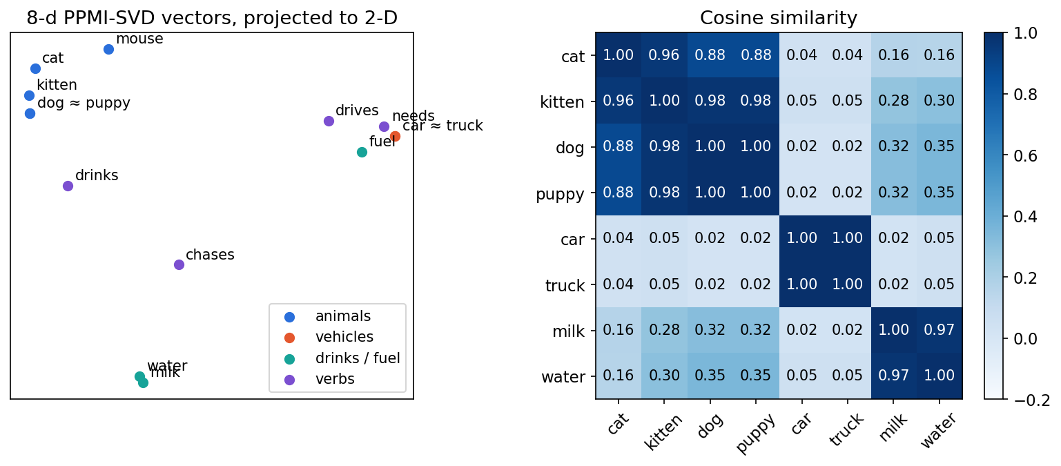
SVD identifies shared patterns across rows rather than assigning a semantic name to each coordinate. The compression cannot preserve every cell when the original matrix has higher rank than . The following synthetic corpus lets us inspect both the construction and a failure of interpreting cosine similarity as synonymy.
Code · Python · 37 lines
import numpy as np

sentences = """the cat drinks milk . the dog drinks water . a cat chases a mouse .
a dog chases a cat . the kitten drinks milk . the puppy drinks water .
a kitten chases a ball . a puppy chases a ball . the car needs fuel .
the truck needs fuel . a car drives on the road . a truck drives on the road .""".split(".")
tokens = [s.split() for s in sentences if s.strip()]
vocab = sorted({w for s in tokens for w in s})
idx = {w: i for i, w in enumerate(vocab)}

# 1) Co-occurrence counts within a +-2 word window.
C = np.zeros((len(vocab), len(vocab)))
for s in tokens:
    for i, w in enumerate(s):
        for j in range(max(0, i - 2), min(len(s), i + 3)):
            if j != i:
                C[idx[w], idx[s[j]]] += 1

# 2) Positive pointwise mutual information.
total = C.sum()
pw, pc = C.sum(1, keepdims=True) / total, C.sum(0, keepdims=True) / total
with np.errstate(divide="ignore"):
    pmi = np.log((C / total) / (pw * pc))
ppmi = np.maximum(pmi, 0)

# 3) Truncated SVD gives dense 8-dimensional embeddings.
U, S, _ = np.linalg.svd(ppmi)
E = U[:, :8] * S[:8]
E /= np.linalg.norm(E, axis=1, keepdims=True)

def nearest(word, k=3):
    sims = E @ E[idx[word]]
    order = [vocab[i] for i in np.argsort(-sims) if vocab[i] != word]
    return [(w, round(float(sims[idx[w]]), 2)) for w in order[:k]]

for w in ["cat", "puppy", "truck", "milk"]:
    print(w, "->", nearest(w))
Output:
Code · 4 lines
cat -> [('kitten', 0.96), ('puppy', 0.88), ('dog', 0.88)]
puppy -> [('dog', 1.0), ('kitten', 0.98), ('cat', 0.88)]
truck -> [('car', 1.0), ('needs', 0.6), ('the', 0.47)]
milk -> [('water', 0.97), ('a', 0.62), ('chases', 0.51)]
Animals cluster with animals and vehicles with vehicles, learned from twelve sentences and no labels. Note “milk” and “water” are nearly identical: both are things that are drunk in this corpus. Embedding similarity measures shared contexts, which often but not always matches similar meaning; antonyms such as “hot” and “cold” also share contexts.
Word2Vec: learn a word by predicting its neighbors
Plain version. Words used in similar surroundings often serve similar roles. Word2Vec turns that observation into a small prediction problem: learn vectors that help recover a word from its neighbors, or its neighbors from the word. The vectors are learned parameters, not hand-written lists of meanings. The two basic architectures are continuous bag of words (CBOW) and Skip-gram [7].
Turn a sentence into training examples
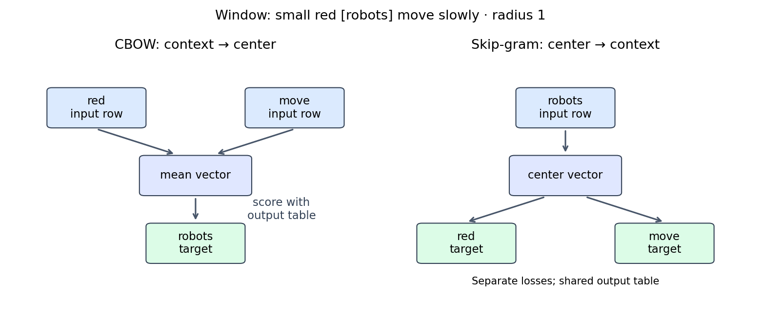
Start with the invented sentence small red robots move slowly. A context window chooses nearby positions; radius one means the word immediately before and after the center. For this example, use only interior centers, so every window has two neighbors:
| Center | Context | CBOW training example | Skip-gram training examples |
|---|---|---|---|
red | small, robots | [small, robots] → red | red → small; red → robots |
robots | red, move | [red, move] → robots | robots → red; robots → move |
move | robots, slowly | [robots, slowly] → move | move → robots; move → slowly |
CBOW combines several context words to predict one center word. Skip-gram uses one center word to predict each context word separately. Skip-gram does not generate an ordered sentence, and “skip” does not mean remove random words. The target may come from either side of the center. At sentence boundaries, an implementation can use shorter windows; our code omits those centers to keep the tensor shapes simple.
The training labels come from the text itself. Nobody must annotate robots with a semantic category before these examples can be created. Repeated occurrences create repeated evidence. The chosen window determines what relationships the model is encouraged to capture: changing it changes the training task, even when the vocabulary stays the same.
Two embedding tables and a softmax
A word needs a vector when it is an input and a vector when it is a prediction candidate. Use two learned tables, rather than assuming these roles share weights:
Here is the input embedding table, is the output embedding table, is vocabulary size, is vector dimension, is a word ID, and the colon selects all coordinates in its row. The transpose makes and column vectors. The vector represents the input, is the target word ID, indexes a candidate word, and is its softmax probability. Each dot product is a prediction score; the denominator makes probabilities sum to one over the vocabulary.
CBOW forms the input by averaging the context vectors. Its loss asks the model to assign high probability to the observed center:
Here is the center word at position , is the set of selected neighboring positions excluding , is its size, is their mean vector, contains the valid center positions, and is the average negative log probability of those centers. The mean ignores context order: exchanging left and right neighbors produces the same input. Some formulations sum context vectors instead; this lesson and its code use the mean.
Skip-gram instead looks up the center vector and applies the same prediction rule to each neighbor:
Here is the Skip-gram loss, is the collection of observed center–context position pairs, is its size, indexes a center position, indexes one neighboring position, is the input word and is its target. Occurrences remain separate even when their word IDs repeat.
A training step increases the observed target’s score relative to competing candidates. It changes both the selected input vectors and the output vectors. Over many examples, reusing the same input row makes the model reconcile that word’s different surroundings. This shared prediction task is the route from discrete word IDs to learned continuous features. Neither architecture needs a deep stack of hidden layers in this basic form, which is the main computational difference from the neural language model in NLP 03.
Negative sampling: compare observed pairs with random draws
A full softmax scores every vocabulary word for every prediction. Negative sampling replaces that vocabulary-wide classification with a smaller binary task: distinguish an observed center–context pair from pairs formed with randomly drawn target words. It was introduced in the Word2Vec follow-up paper [8].
For an observed input word and context word , one sampled loss is:
Here is the negative-sampling loss for one observed pair, is the center word ID, is its observed context word ID, is the center’s input vector, and are output vectors, is the chosen number of random targets, is draw from distribution , and is the sigmoid applied to a real score . The first term rewards a large observed-pair score; the remaining terms reward small random-pair scores. The full training objective averages this expression over observed pairs and sampling randomness. For a CBOW version, use the averaged context vector in place of .
A common sampling distribution from the original paper is:
Here is the probability of drawing vocabulary word , is its corpus occurrence count, indexes vocabulary entries, and is vocabulary size. The exponent flattens the frequency distribution relative to sampling directly by counts. It is a design choice, not a universal probability law.
For the observed pair robots → move, a random draw might create robots → red. The label “negative” means drawn by the noise process; it does not assert that the two words can never occur together. A draw can be a genuine context elsewhere, or even collide with this target. An implementation must specify whether it retains, skips or redraws collisions; changing that rule changes the sampled objective. The model separates statistical sources of pairs rather than learning a dictionary of absolute incompatibilities.
The binary sigmoid scores do not sum to one over vocabulary words. Negative sampling is a different training objective, not an exact computation of the softmax above, and its loss is not a normalized next-token likelihood. Use it to learn useful representations; evaluate those representations on the intended downstream task.
Why prediction changes vector geometry
The phrase “learn from neighbors” becomes concrete in the gradient. For one full-softmax target, let its score be the dot product between an output vector and the input representation:
Here is candidate ‘s score, is the loss for observed target , equals one for that target and zero otherwise, and is the gradient with respect to the input representation. The embedding tables, vocabulary size and conditional probability are those defined above.
Gradient descent moves the input toward the observed output vector and away from the model’s probability-weighted average of alternatives. A word with many occurrences receives many such updates through the same row. Similar context distributions can therefore give different words compatible predictive roles, without any training label declaring them synonyms.
For mean-based CBOW, every selected context row receives . The input cannot distinguish two contexts that are permutations of the same words. For Skip-gram, one center row receives updates from multiple neighbor targets. Its basic score has no slot for whether a neighbor was on the left or right. Choosing the window therefore chooses which relations the objective can directly represent; a wider window is not simply a more accurate version of a narrow one.
What negative-sampling scores estimate
We can inspect the sampling objective before imposing the embedding dimension. Fix a center word and imagine that every candidate has an independently adjustable score. Let be its empirical context probability and its noise probability. The expected contribution for that candidate is:
Here is one candidate context, is its unrestricted real score, and are the two probabilities for the fixed center, is the number of independent noise draws per observed pair and is the sigmoid defined above. This calculation retains collisions between noise draws and observed targets.
When both probabilities are positive, the stationary score is:
Here minimizes that candidate’s expected loss. For , and , it is zero: half the relevant probability mass is attributed to each statistical source. If instead, the optimum becomes . The observed context frequency stayed fixed; the noise distribution changed the score. A positive score therefore means “more associated than this sampling baseline,” rather than “the pair is certainly meaningful.” If the observed probability is zero and noise probability is positive, the unrestricted optimum tends toward negative infinity.
When noise is exactly the corpus context marginal, this ratio yields PMI minus . Levy and Goldberg analyze the resulting matrix-factorization interpretation [9]. The common three-quarter-power distribution changes the ratio. In an actual embedding model, scores share low-dimensional vectors, so they cannot generally reach every independent optimum. The learned tables compromise among the pair statistics under a rank constraint. This explains both the connection to the count-based construction and why truncating a PPMI matrix and training Word2Vec need not give identical vectors.
Full softmax costs roughly arithmetic per target, while scoring one observed target and draws costs , before sampling and batching overhead. Here is embedding dimension. The saving comes with a different objective. Neither the sigmoid value nor the negative-sampling loss is a substitute for the normalized token probability used to report perplexity.
Train CBOW and Skip-gram on CPU
This standalone example learns both input and output tables using full softmax. The vocabulary is tiny, so we can inspect the objective without a sampling approximation. Both models use the same invented corpus, radius-one interior windows, embedding width and training loop. A one-token input average in the Skip-gram path is simply the center vector.
Code · Python · 57 lines
import torch
from torch import nn
from torch.nn import functional as F

torch.manual_seed(7)
torch.set_num_threads(1)
corpus = [
    'small red robots move slowly',
    'small blue robots move quickly',
    'large red sensors work slowly',
    'large blue sensors work quickly',
    'small red sensors work quietly',
    'large blue robots move quietly',
]
vocab = sorted(set(' '.join(corpus).split()))
ids = {word: i for i, word in enumerate(vocab)}
cbow_x, cbow_y, sg_x, sg_y = [], [], [], []
for sentence in corpus:
    tokens = [ids[word] for word in sentence.split()]
    # Use radius 1 and interior centers, so every context has two words.
    for t in range(1, len(tokens) - 1):
        neighbors = [tokens[t - 1], tokens[t + 1]]
        cbow_x.append(neighbors)
        cbow_y.append(tokens[t])
        for neighbor in neighbors:
            sg_x.append([tokens[t]])
            sg_y.append(neighbor)

class Word2Vec(nn.Module):
    def __init__(self, size, width=8):
        super().__init__()
        self.input = nn.Embedding(size, width)
        self.output = nn.Embedding(size, width)
        nn.init.normal_(self.input.weight, std=0.1)
        nn.init.normal_(self.output.weight, std=0.1)

    def forward(self, context):
        h = self.input(context).mean(dim=1)
        return h @ self.output.weight.T

embeddings = {}
for name, inputs, targets in [('CBOW', cbow_x, cbow_y),
                             ('Skip-gram', sg_x, sg_y)]:
    x, y = torch.tensor(inputs), torch.tensor(targets)
    model = Word2Vec(len(vocab))
    optimizer = torch.optim.SGD(model.parameters(), lr=1.0)
    initial = F.cross_entropy(model(x), y).item()
    for step in range(250):
        optimizer.zero_grad()
        loss = F.cross_entropy(model(x), y)
        loss.backward()
        optimizer.step()
    final = F.cross_entropy(model(x), y).item()
    assert final < initial
    embeddings[name] = model.input.weight.detach().clone()
    print(name, len(y), f'{initial:.3f} -> {final:.3f}')
print('vocabulary', len(vocab), 'embedding shape', tuple(embeddings['CBOW'].shape))
The run prints CBOW 18 2.384 -> 0.159, Skip-gram 36 2.402 -> 1.198, and vocabulary 11 embedding shape (11, 8). Losses are mean negative log probabilities in nats. The assertions establish that the implementation fits these training examples. The smaller CBOW loss does not establish that CBOW produces better word vectors: its targets and conditional inputs differ from Skip-gram’s. This corpus is too small to judge semantic neighborhoods or natural-language generalization.
After training, embeddings['CBOW'][ids['robots']] retrieves one learned input vector. The output table was needed to train it but can be omitted when serving a downstream model that only looks up input vectors. Record which table you retain; using input vectors, output vectors or a combination is a representation choice.
Optional: word2vec (in the Paper guides). Follow the original figure, objective, experimental comparisons and limitations.
GloVe: fit log co-occurrence counts directly
Plain version. Instead of streaming through windows one prediction at a time, GloVe first counts how often every pair of words co-occurs, then fits word vectors whose dot products reproduce the logarithms of those counts. Frequent pairs get more weight, but not unlimited weight.
Pennington et al. motivate GloVe with ratios of co-occurrence probabilities [10]. Let be the (distance-weighted) number of times word occurs in the context of word , and . For two words and , the ratio is large for context words that belong with but not , small for the reverse, and near one for words that are equally related or unrelated to both. The ratio discriminates better than either probability alone. The model asks vector differences to encode such ratios, which leads to a weighted least-squares objective over the co-occurrence matrix:
Here is vocabulary size, is the co-occurrence count of words and , is the word vector of , is a separate context vector of , and are scalar biases, is a weighting function, and and are its cutoff and exponent. Because , cells with zero count contribute nothing, so is never needed and the sum runs only over observed pairs. The paper fixes and , uses a co-occurrence weighting in which a pair words apart adds , and reports the sum of the two tables as the final word vectors [10].
Three design choices separate GloVe from Word2Vec. It trains on global counts rather than on individual windows, so one pass over the corpus builds and training then costs time proportional to the number of nonzero cells. The biases absorb word frequency, so the dot product models what remains. And the weighting function prevents very frequent pairs, such as those involving the, from dominating, while giving rare and noisy pairs little influence. Like negative sampling, the objective factorizes a shifted log-count matrix under a rank constraint, which is why GloVe and Skip-gram vectors often behave similarly in practice.
The following code computes the ingredients on the earlier toy corpus: co-occurrence ratios and the weighting function.
Code · Python · 27 lines
import numpy as np

text = """the cat drinks milk . the dog drinks water . a cat chases a mouse .
a dog chases a cat . the kitten drinks milk . the puppy drinks water .
a kitten chases a ball . a puppy chases a ball . the car needs fuel .
the truck needs fuel . a car drives on the road . a truck drives on the road ."""
sents = [s.split() for s in text.split(".") if s.strip()]
vocab = sorted({w for s in sents for w in s})
idx = {w: i for i, w in enumerate(vocab)}

X = np.zeros((len(vocab), len(vocab)))            # +-2 window, 1/distance weighting
for s in sents:
    for i, w in enumerate(s):
        for j in range(max(0, i - 2), min(len(s), i + 3)):
            if j != i:
                X[idx[w], idx[s[j]]] += 1.0 / abs(i - j)
P = X / X.sum(1, keepdims=True)                   # P(k | i): row-normalized counts

for k in ["drinks", "chases", "needs", "the"]:
    a, b = P[idx["kitten"], idx[k]], P[idx["truck"], idx[k]]
    ratio = "inf" if b == 0 else f"{a / b:.2f}"
    print(f"P({k}|kitten)={a:.3f}  P({k}|truck)={b:.3f}  ratio={ratio}")

def f(x, x_max=100.0, alpha=0.75):                 # GloVe weighting function
    return np.minimum((x / x_max) ** alpha, 1.0)
print("f at 1, 10, 100, 1000:", np.round(f(np.array([1.0, 10.0, 100.0, 1000.0])), 3))
print("nonzero cells:", int((X > 0).sum()), "of", X.size)
The run prints:
Code · 6 lines
P(drinks|kitten)=0.200  P(drinks|truck)=0.000  ratio=inf
P(chases|kitten)=0.200  P(chases|truck)=0.000  ratio=inf
P(needs|kitten)=0.000  P(needs|truck)=0.200  ratio=0.00
P(the|kitten)=0.200  P(the|truck)=0.200  ratio=1.00
f at 1, 10, 100, 1000: [0.032 0.178 1.    1.   ]
nonzero cells: 96 of 361
The ratios separate animal contexts from vehicle contexts, while the gives a ratio of one and therefore no information. The output also exposes a limitation of this tiny corpus: almost three quarters of the matrix is zero, and GloVe ignores zero cells. With so few observed pairs, a model with a few hundred parameters can fit every observed cell exactly, and the resulting geometry depends mainly on initialization. GloVe’s count-based design needs large corpora in which the matrix is well populated; we therefore do not train it here. Exercise 3 asks you to observe this underdetermination yourself.
Optional: GloVe (in the Paper guides). Follow the original figure, objective, experimental comparisons and limitations.
fastText: vectors from character n-grams
Plain version. A word-level table has no vector for a word it never saw, and it treats charger and chargers as unrelated rows. fastText builds each word’s vector from vectors of its character pieces, so related spellings share parameters and unseen words still get a vector.
Bojanowski et al. extend Skip-gram with negative sampling by representing each word as a bag of character n-grams [11]. The word is wrapped in boundary symbols, < and >, so that prefixes and suffixes are distinguishable from the same letters inside a word, and the whole wrapped word is added as one extra unit. In the paper, all n-grams with are used. The score between a center word and a context word becomes
Here is the set of n-grams of (including the wrapped word itself), is the learned vector of n-gram , and is the context vector of . The word’s own vector is . This score replaces in the negative-sampling loss above. To bound memory, the paper maps n-grams into a fixed number of buckets with a hash function, so unrelated n-grams can share a vector [11].
Code · Python · 25 lines
import numpy as np

def char_ngrams(word, n_min=3, n_max=6):
    w = f"<{word}>"                       # boundary symbols mark prefixes and suffixes
    grams = {w[i:i + n] for n in range(n_min, n_max + 1) for i in range(len(w) - n + 1)}
    return grams | {w}                    # the whole word is kept as one extra unit

print(sorted(char_ngrams("robot", 3, 3)))
vocab = ["charge", "charger", "recharge", "discharge", "robot", "robots"]
query = "chargers"                        # not in the vocabulary
q = char_ngrams(query)
for word in vocab:
    print(f"{word:10s} shares {len(q & char_ngrams(word)):2d} of {len(q)} units with '{query}'")

# A fastText-style vector is the sum of its unit vectors, so an unseen word still gets one.
rng = np.random.default_rng(0)
table = {}                                # stands in for a trained (hashed) n-gram table
def vector(word, dim=8):
    return sum(table.setdefault(g, rng.normal(size=dim)) for g in sorted(char_ngrams(word)))
def cos(a, b):
    return a @ b / (np.linalg.norm(a) * np.linalg.norm(b))
for word in vocab:
    vector(word)
print("cos(chargers, charger) =", round(cos(vector("chargers"), vector("charger")), 3))
print("cos(chargers, robots)  =", round(cos(vector("chargers"), vector("robots")), 3))
The run prints:
Code · 9 lines
['<ro', '<robot>', 'bot', 'obo', 'ot>', 'rob']
charge     shares 14 of 27 units with 'chargers'
charger    shares 18 of 27 units with 'chargers'
recharge   shares 10 of 27 units with 'chargers'
discharge  shares 10 of 27 units with 'chargers'
robot      shares  0 of 27 units with 'chargers'
robots     shares  0 of 27 units with 'chargers'
cos(chargers, charger) = 0.804
cos(chargers, robots)  = -0.222
The n-gram vectors here are random, not trained, so the high cosine between chargers and charger comes only from the units they share. That is exactly the mechanism: an unseen inflection inherits most of its vector from known pieces. Training decides whether sharing is helpful. It usually is for inflection and derivation, and it is misleading for words that share letters by accident; discharge and recharge share charge but differ in meaning in ways the pieces do not reveal. Subword vectors help most for morphologically rich languages and for rare words. Note the relation to the subword tokenizers in NLP 02: BPE splits a word into one sequence of pieces before lookup, whereas fastText sums vectors of all overlapping n-grams.
Dense word and document representations
Plain version. A dense vector lets different words share statistical strength. That can connect related phrases, but the vector’s geometry reflects its training data and objective rather than a universal definition of meaning.
Static vectors provide compact reusable features for a classifier, nearest-neighbor word exploration or a pooled document baseline. They are useful when a labeled application has little data but an appropriate text corpus is available. Training the embedding and the downstream classifier are different stages: neighbor prediction never directly learns a billing label or an abstention policy.
A static embedding table assigns a vector to each vocabulary entry:
Here is the embedding table, is vocabulary size, is embedding dimension, is the token ID at position , is its row vector, is document length in tokens and is the mean-pooled document vector. The colon denotes all coordinates in the selected row.
The tables above supply ways to obtain . Once token vectors are available, mean pooling turns a variable-length document into a fixed-width feature. This aggregation step is separate from the objective used to train the table.
Mean pooling is an instructive baseline because it exposes a limitation clearly. Any permutation of a document’s tokens gives the same average. The representation of “the technician helped the customer” is identical to “the customer helped the technician” if the same static token vectors are used. It also treats negation as one contribution among many rather than an operator changing the meaning of a phrase. The word bank retrieves the same static vector in river bank and bank account; more training data does not change this lookup rule.
There are two separate choices: how token vectors are obtained and how they are combined. You can freeze pretrained token vectors and train only a classifier, fine-tune the vectors with the classifier, or train all parameters from scratch. Freezing reduces the number of task-specific parameters. Fine-tuning can adapt meanings to a domain, but small datasets can distort representations or memorize labels.
Do not compare embeddings only by visually attractive clusters. A two-dimensional projection can conceal overlap in the original space. Compare representations under the same task, split, classifier capacity and tuning allowance. If a dense representation changes the downstream head too, the experiment no longer isolates the representation.
Cosine measures direction, not truth
The count-based example compares unit-normalized vectors. Its dot product is then the cosine of the angle between them:
Here and are nonzero embedding column vectors, is their inner product, and is Euclidean length. The cosine lies between and . A zero vector needs an explicit handling rule because the denominator vanishes.
Cosine removes positive rescaling of either vector. It does not remove every transformation compatible with the training objective. In the two-table model, the predictive scores depend on products of an input and an output vector. Many different tables produce the same products:
Here and are the input and output tables with shape , is any invertible matrix, is the transpose of its inverse, and and are the transformed tables. Each cell of is one center–output prediction score. Thus full-softmax predictions and the negative-sampling objective are unchanged by this paired transformation. The same argument applies to GloVe’s .
An orthogonal change of coordinates preserves input-vector angles, but general invertible changes need not. Consequently, identical prediction loss does not uniquely determine cosine neighborhoods in the retained input table. Optimization, initialization and additional constraints select a particular solution. This is one reason a low training loss alone cannot certify useful downstream similarity.
This standalone numerical check combines three claims: score preservation, order invariance of averaging, and the noise-dependent optimum derived above. The matrices are hand-chosen for this calculation; they are not trained language vectors.
Code · Python · 28 lines
import numpy as np

# Two input rows and three output rows: scores are center-output dot products.
E = np.array([[1., 1.], [1., -1.]])
U = np.array([[1., 0.], [0., 1.], [-1., 1.]])
A = np.diag([2., 0.5])
changed_E = E @ A
changed_U = U @ np.linalg.inv(A).T

def cosine(a, b):
    return (a @ b) / (np.linalg.norm(a) * np.linalg.norm(b))

assert np.allclose(E @ U.T, changed_E @ changed_U.T)
assert np.allclose(E[[0, 1]].mean(0), E[[1, 0]].mean(0))
print('scores unchanged:', np.allclose(E @ U.T, changed_E @ changed_U.T))
print('cosine:', f'{cosine(E[0], E[1]):.3f}', '->',
      f'{cosine(changed_E[0], changed_E[1]):.3f}')
print('mean unchanged by order:',
      np.allclose(E[[0, 1]].mean(0), E[[1, 0]].mean(0)))

# The unrestricted negative-sampling optimum depends on the noise baseline.
p, K = 0.5, 2
for q in [0.25, 0.05]:
    score = np.log(p / (K * q))
    sigmoid = 1 / (1 + np.exp(-score))
    gradient = (p + K * q) * sigmoid - p
    assert np.isclose(gradient, 0)
    print('noise', q, 'optimal score', f'{score:.3f}')
The output is:
Code · 5 lines
scores unchanged: True
cosine: 0.000 -> 0.882
mean unchanged by order: True
noise 0.25 optimal score 0.000
noise 0.05 optimal score 1.609
The cosine changed while all center–output scores stayed fixed. The equal means have a different implication: once a representation merges two token orders, no classifier that receives only that mean can recover which order occurred. These are properties of the representation, rather than evidence that one optimizer ran poorly.
Evaluating word embeddings
Plain version. There are two ways to judge embeddings: ask whether their geometry agrees with human judgments about words (intrinsic), or plug them into a task and measure the task (extrinsic). Neither alone tells you whether vectors are “good.”
Similarity: correlate cosines with human ratings
A word-similarity dataset lists word pairs with graded human ratings. The model scores each pair by cosine, and the evaluation measures how well the two rankings agree with Spearman’s rank correlation:
Here is the number of pairs, is the difference between the rank of pair under the model’s cosines and its rank under the human ratings, and . This formula assumes no ties; with ties, is the Pearson correlation of the ranks. Spearman’s uses only ranks, so it ignores the scale of cosines.
What the ratings mean matters as much as the statistic. WordSim-353 is a widely used set of rated word pairs [12]. Hill et al. point out that its ratings do not separate similarity from association, and built SimLex-999 to quantify similarity explicitly, so that associated but dissimilar pairs receive low ratings [13]. A model trained with broad windows may score well on association-style data and poorly on similarity-style data, for the reason given in the lexical-semantics section: distributional evidence mixes the relations.
Analogy: the vector-offset test and its caveats
Mikolov, Yih and Zweig observed that some relations appear as roughly constant vector offsets [14]. To answer “ is to as is to ?”, the offset method returns
Here is the vocabulary, is the vector of candidate , and the three question words are excluded from the candidates. Linzen points out that this exclusion is doing real work: the target point often lies closest to itself, so the method’s success mixes offset consistency with the neighborhood structure around [15]. He recommends reporting simple baselines, such as returning the nearest neighbor of , alongside analogy accuracy.
The next example evaluates the PPMI vectors from earlier with invented similarity ratings and three analogies. The ratings are made up for this lesson and are not a benchmark.
Code · Python · 41 lines
import numpy as np
from scipy.stats import spearmanr

text = """the cat drinks milk . the dog drinks water . a cat chases a mouse .
a dog chases a cat . the kitten drinks milk . the puppy drinks water .
a kitten chases a ball . a puppy chases a ball . the car needs fuel .
the truck needs fuel . a car drives on the road . a truck drives on the road ."""
sents = [s.split() for s in text.split(".") if s.strip()]
vocab = sorted({w for s in sents for w in s})
idx = {w: i for i, w in enumerate(vocab)}
C = np.zeros((len(vocab), len(vocab)))
for s in sents:
    for i, w in enumerate(s):
        for j in range(max(0, i - 2), min(len(s), i + 3)):
            if j != i:
                C[idx[w], idx[s[j]]] += 1
P = C / C.sum()
with np.errstate(divide="ignore"):
    ppmi = np.maximum(np.log(P / (P.sum(1, keepdims=True) * P.sum(0, keepdims=True))), 0)
U, S, _ = np.linalg.svd(ppmi)
E = U[:, :8] * S[:8]
E /= np.linalg.norm(E, axis=1, keepdims=True)
cos = lambda a, b: float(E[idx[a]] @ E[idx[b]])

# 1) Similarity: correlate model cosines with (invented) graded judgments, 0-10.
judged = [("cat", "kitten", 9), ("dog", "puppy", 9), ("car", "truck", 8), ("milk", "water", 5),
          ("cat", "dog", 6), ("cat", "mouse", 3), ("car", "road", 2), ("kitten", "fuel", 0)]
model = [cos(a, b) for a, b, _ in judged]
rho = spearmanr(model, [h for _, _, h in judged]).statistic
print(f"Spearman rho = {rho:.3f} over {len(judged)} pairs")

# 2) Analogy a:b :: c:? with the offset b - a + c (3CosAdd).
def analogy(a, b, c, exclude_inputs=True):
    target = E[idx[b]] - E[idx[a]] + E[idx[c]]
    scores = E @ (target / np.linalg.norm(target))
    for i in np.argsort(-scores):
        if not exclude_inputs or vocab[i] not in (a, b, c):
            return vocab[i]
for a, b, c in [("cat", "kitten", "dog"), ("car", "fuel", "cat"), ("cat", "milk", "puppy")]:
    print(f"{a}:{b} :: {c}:?  ->", analogy(a, b, c), "| without excluding inputs ->",
          analogy(a, b, c, exclude_inputs=False))
The run prints:
Code · 4 lines
Spearman rho = 0.837 over 8 pairs
cat:kitten :: dog:?  -> puppy | without excluding inputs -> puppy
car:fuel :: cat:?  -> kitten | without excluding inputs -> cat
cat:milk :: puppy:?  -> water | without excluding inputs -> water
Two analogies come out as intended. The middle one shows both caveats at once. Without exclusion, the answer is cat, one of the question words. With exclusion, the answer is kitten, the nearest neighbor of cat, not milk, the intended “what it consumes” answer. The offset did not carry the relation; the neighborhood of decided. Eight invented pairs and three analogies are, of course, far too few to support any general claim about these vectors.
Intrinsic versus extrinsic
Schnabel et al. compare evaluation methods and find that different evaluations order embedding methods differently, that word frequency affects results and cosine similarity, and that extrinsic tasks should not be used as a proxy for generic embedding quality [16]. The practical rule is to evaluate on the relation your application needs.
Nearest-neighbor lists can reveal obvious corpus patterns, but they are a diagnostic rather than an application score. Separate lexical questions: is the candidate a synonym, an antonym, a word associated with the topic, or a word that can occupy the same grammatical slot? A single unqualified notion of “related” hides these distinctions.
Use controlled pairs alongside ordinary held-out examples. For a representation used in sentiment, compare a positive claim with its negation. For a role-sensitive task, exchange who acted on whom while holding the word inventory fixed. For a technical corpus, test a term used in its domain-specific and everyday senses. These tests ask whether the representation preserves a required difference; they do not demand that every word pair occupy a predetermined location.
If mean pooling makes a critical pair identical, collecting more classifier labels cannot fix that collision while the representation remains fixed. If the vectors distinguish the pair but the classifier predicts incorrectly, supervision or the decision boundary may be responsible. Locate the failure at the earliest stage that loses the needed evidence.
Bias in embeddings
Plain version. Embeddings learn whatever regularities the corpus contains, including social stereotypes. If a group of names co-occurs with some occupations more than others, the vectors encode that association, and downstream systems can reproduce it.
Bolukbasi et al. showed that word embeddings trained on news text encode gender stereotypes, identified a gender direction in the space, and proposed removing it from words that should be gender-neutral [17]. Caliskan et al. introduced the Word Embedding Association Test (WEAT), modeled on the Implicit Association Test from psychology, and found that embeddings reproduce a range of documented human biases [18]. For a target word and two attribute sets and , the association used by WEAT is
Here and are the set sizes and denotes word vectors. A positive value means is closer on average to set . The full test aggregates this score over two sets of target words and compares it with a permutation distribution.
The following invented corpus contains no sentence linking a name to an occupation. Occupation words always appear with their own activity, while invented names appear with activities at skewed rates.
Code · Python · 47 lines
import random
import numpy as np

rng = random.Random(0)
# An invented corpus. Job words always appear with their own activity; invented
# names appear with activities at skewed rates. No sentence says "ana is a pilot".
group_a, group_b = ["ana", "ari"], ["bo", "bea"]
activity = {"pilot": "flies the plane", "baker": "bakes the bread", "clerk": "files the forms"}
share_a = {"pilot": 0.8, "baker": 0.2, "clerk": 0.5}    # P(group A | activity)
sents = []
for _ in range(3000):
    job = rng.choice(list(activity))
    if rng.random() < 0.5:
        sents.append(f"the {job} {activity[job]}".split())
    else:
        name = rng.choice(group_a if rng.random() < share_a[job] else group_b)
        sents.append(f"{name} {activity[job]}".split())
vocab = sorted({w for s in sents for w in s})
idx = {w: i for i, w in enumerate(vocab)}
C = np.zeros((len(vocab), len(vocab)))
for s in sents:
    for i, w in enumerate(s):
        for j in range(max(0, i - 2), min(len(s), i + 3)):
            if j != i:
                C[idx[w], idx[s[j]]] += 1
P = C / C.sum()
with np.errstate(divide="ignore"):
    ppmi = np.maximum(np.log(P / (P.sum(1, keepdims=True) * P.sum(0, keepdims=True))), 0)
U, S, _ = np.linalg.svd(ppmi)
E = U[:, :4] * S[:4]
E /= np.linalg.norm(E, axis=1, keepdims=True)

def association(word, E):            # mean cosine to group A minus mean cosine to group B
    unit = E / np.linalg.norm(E, axis=1, keepdims=True)
    w = unit[idx[word]]
    return np.mean([w @ unit[idx[a]] for a in group_a]) - np.mean([w @ unit[idx[b]] for b in group_b])

for job in activity:
    print(f"{job:6s} association {association(job, E):+.3f}")

# Project out one "group direction" and measure again.
d = E[[idx[a] for a in group_a]].mean(0) - E[[idx[b] for b in group_b]].mean(0)
d /= np.linalg.norm(d)
E_proj = E.copy()
for job in activity:
    E_proj[idx[job]] -= (E_proj[idx[job]] @ d) * d
print("after projection:", [f"{job} {round(association(job, E_proj), 3) + 0.0:+.3f}" for job in activity])
The run prints:
Code · 4 lines
pilot  association +0.795
baker  association -0.811
clerk  association +0.072
after projection: ['pilot +0.000', 'baker +0.000', 'clerk +0.000']
The skew in who performs which activity became a strong association between names and occupation words, even though the two never co-occur in a sentence: both share the activity contexts. Projecting out the group direction sets the measured association to zero, but that result is circular, because the projection removes exactly the direction this score measures. Gonen and Goldberg show that, for published debiasing methods, the bias is largely hidden rather than removed: it remains in the distances between supposedly neutralized words and can be recovered from them [19]. Treat a debiasing step as one intervention to be audited on the downstream task, not as a guarantee, and remember that the source of the association is the data.
From word vectors to sentence embeddings
Plain version. An embedding supplies features; an application still needs a target, supervision and an action rule. When the application compares whole sentences, train the sentence representation for the comparison it will support.
For document classification, mean pooling is a convenient first experiment. Build one vector per training document, fit a classifier on its labels, and apply the same tokenizer, embedding lookup and pooling at evaluation time. Compare it with the sparse features and convolutional encoders developed in NLP 03. Keep the data split and classifier tuning allowance fixed so that a change in representation can be assessed fairly.
A frozen table uses contextual statistics learned before the labeled task. Fine-tuning lets the labels adjust the rows. These policies answer different questions: whether reusable corpus features already distinguish the classes, and whether task-specific changes improve them. With limited labels, fine-tuning can also fit incidental identifiers. Holding out groups such as conversations or repeated document templates helps reveal that behavior.
Decide how to handle uncovered text. Mapping every unknown word to one row merges all such words. Dropping them changes the pooling denominator and may leave an empty document. Returning a zero vector does not create a meaningful cosine direction. Subword vectors reduce but do not remove this problem. Coverage, the number of retained tokens, and the action for an empty representation are part of the model specification.
For word-level tagging, retain the sequence of token vectors rather than pooling it into one document vector. A downstream encoder can then combine local context before predicting a label per position. This does not make the original table contextual: the initial lookup of bank is still identical in both senses. The context-dependent computation happens afterward.
Similarity and contrastive sentence learning
A representation useful for predicting neighboring words may need adaptation before distances between whole sentences become reliable. Sentence-BERT trains paired sentence representations with a shared encoder and task objectives, making sentence comparisons possible without jointly encoding every candidate pair [20]. The computational distinction matters: separately cached document vectors can support retrieval, whereas a model that reads a query and candidate together must run for each pair.
A generic contrastive objective makes the intended geometry explicit:
Here is the loss for one query, is its vector, is the vector of a relevant paired text included among the candidates, is candidate , is candidate count and is a temperature controlling the sharpness of the distribution. This is a generic learning construction, not a claim that every sentence encoder uses this exact objective. It has the same shape as the Word2Vec softmax: one observed pair competes with alternatives.
SimCSE is a widely used instance [21]. Its unsupervised version encodes the same sentence twice; because dropout differs between the two passes, the two vectors differ slightly and form a positive pair, while other sentences in the batch are negatives. The authors report that removing dropout leads to representation collapse. Its supervised version uses natural-language-inference data, taking entailment pairs as positives and contradiction pairs as hard negatives [21].
Negative examples define what “different” means. Two tickets about different invoices might be useful negatives for finding the same case but poor negatives for recognizing the billing category. False negatives can push semantically related examples apart. Before changing an encoder, inspect how positive and negative pairs are sampled.
Similarity also differs from entailment. “The parcel arrived” and “The parcel did not arrive” share topic and many tokens. They may be close in a semantic search space while making opposite claims. Classification, semantic search and inference therefore require different validation examples, even when they share an encoder. NLP 11 treats inference as its own task.
Preview: contextual embeddings
Plain version. A static table gives bank one vector everywhere. A contextual model computes a different vector for each occurrence, using the surrounding words, so the river sense and the money sense can come apart.
Peters et al. compute ELMo representations as functions of the entire input sentence, using the internal states of a bidirectional language model, and add them as features to task models [22]. BERT takes the step further within its pretrained encoder: a token’s final hidden state depends on the other permitted input tokens [23]. The distinction is lookup versus computation. Both systems may begin with an embedding table; static Word2Vec exposes a row directly, while BERT processes rows and positions through a context-dependent network.
Context can improve sense discrimination, but it does not turn every hidden-state cosine into a calibrated similarity measure. A static vector is a type-level summary across many occurrences; a contextual vector is a token-level representation of one occurrence. Which one an application needs depends on whether it asks about a word in general or a word as used here. NLP 07 builds the attention mechanism these models use, and NLP 10 develops masked pretraining and BERT’s contextual representations rather than repeating them here.
Modern view
Turney and Pantel’s survey [6] distinguishes term–document, word–context and pair–pattern matrices. Its taxonomy makes the source of evidence explicit: a document association, a neighboring-word relation and a relational pattern are different observations. The lesson here is to define the matrix before interpreting the vector space.
Apidianaki’s 2023 review [24] follows word meaning from static type-level vectors to contextual token-level representations and back. It covers semantic specialization, sense distinctions, representation interpretation and the derivation of static vectors from contextual encoders. Its central distinction is the level at which evidence is aggregated, rather than a ranking in which a newer architecture automatically solves every lexical task. Methods that inject lexical-resource relations into vectors connect directly to the WordNet section of this lesson.
For sentence- and text-level embeddings, Muennighoff et al.’s MTEB benchmark spans 8 embedding tasks, 58 datasets and 112 languages, and its authors find that no single text-embedding method dominates across all tasks [25]. In 2023–2026, most practical text embeddings come from pretrained Transformer encoders or language models fine-tuned with contrastive objectives of the kind shown above, and benchmark suites in the style of MTEB are the usual way to compare them. Static vectors remain useful as fast, transparent baselines, as features in low-resource settings, and as objects of study.
A useful research lens is therefore: what meaning distinction survives this representation, and how was that checked? Contextual hidden states, static vectors obtained by aggregating them, and task-trained sentence representations answer different questions. An embedding that preserves a broad topic may still collapse a negated claim or a rare sense. A small static table can remain an appropriate baseline when its measurable invariances match the application.
Open questions include reliable geometry across domains, sense separation when evidence is sparse, bias that survives debiasing, and comparisons that hold corpus and evaluation conditions fixed. Multilingual work adds segmentation and uneven coverage: a row is only useful if the tokenizer and training corpus supplied evidence for that type. Report those conditions and challenge examples alongside the final score. This keeps the explanation tied to observed language behavior.
Key takeaways
- A vocabulary entry is a form or lemma, not a sense; lexical relations such as synonymy, antonymy and hypernymy hold between senses, and WordNet records them by hand.
- A static embedding aggregates many occurrences into one vector per vocabulary entry; distributional similarity captures shared usage and mixes synonymy, antonymy and relatedness.
- PPMI compares co-occurrence with independence; SVD, Skip-gram with negative sampling and GloVe all compress association statistics under a rank constraint.
- CBOW predicts a center from combined neighbors; Skip-gram predicts neighbors separately; negative sampling distinguishes statistical sources of pairs and is not a normalized distribution.
- fastText builds word vectors from character n-grams, so related spellings share parameters and unseen words get vectors.
- Similarity and analogy tests depend on what the ratings mean and on details such as excluding the question words; evaluate the relation your application needs.
- Embeddings absorb corpus associations, including social biases; projection-based debiasing can hide rather than remove them.
- Mean pooling erases order; sentence embeddings should be trained for the comparison they serve, and contextual models compute a vector per occurrence rather than looking one up.
Exercises
- Build the examples. Enumerate radius-one CBOW and Skip-gram examples for
robots help people today, using only interior centers. Then include the boundary centers. Which input shapes change?
Hint
Count centers separately from center–context pairs. Variable-length CBOW contexts need a mask or separate processing; Skip-gram still receives one center ID per pair.
- Inspect a matrix cell. Construct a corpus in which one context occurs frequently overall but has PMI near zero for a chosen center. Then add observed center–context pairs and explain both the numerator and marginal changes.
Hint
Begin with a joint table close to independence. Recompute all marginals after editing the count; keeping them fixed would analyze a different table.
- Train GloVe and watch it wobble. Implement the GloVe objective in PyTorch on the toy corpus, training only on nonzero cells. Train it with three random seeds and compare the nearest neighbors of
cat. Then count the parameters and the nonzero cells. What explains the instability, and what would make the problem better determined?
Hint
Two tables plus two bias vectors can easily outnumber the observed cells. A larger corpus with more varied contexts adds equations; a smaller removes unknowns.
- Similarity versus relatedness. Write ten word pairs that are related but not similar (such as
cupandcoffee) and ten that are similar. Using the PPMI code with window radius 1 and then 4 on a corpus you write, compare how the cosine separates the two groups.
Hint
Wider windows collect topical co-occurrence, which favors relatedness; narrow windows emphasize words that fill the same slot. Report the change for both groups, not a single score.
- Expose an invariant. Create two meaningful sentences with the same word counts and different participant roles. Show why static mean pooling cannot separate them, even if every word vector is learned perfectly for its training objective.
Hint
Changing order does not change a sum. The limitation holds for every possible static embedding table, not only for the synthetic values in this lesson.
- Audit beyond the projection. In the bias example, after projection, compute each occupation word’s nearest names using all remaining dimensions, and train a small logistic classifier to predict group A versus group B from the projected occupation-word neighbors. Does the association still leave a trace?
Hint
The projection removed one direction measured one way. Look for structure the score did not measure, as Gonen and Goldberg did with clustering and classification.
References
- M. Hagiwara, Real-World Natural Language Processing: Practical Applications with Deep Learning, Manning, 2021; Chapters 3–4. publisher
- S. McRoy, Principles of Natural Language Processing, open textbook, 2021; Chapter 6, “Benchmark Tasks for Language Modelling.” chapter
- Y. Bengio, R. Ducharme, P. Vincent and C. Jauvin, “A neural probabilistic language model,” Journal of Machine Learning Research 3, 2003. paper
- G. A. Miller, “WordNet: a lexical database for English,” Communications of the ACM 38(11), 1995. paper
- Z. S. Harris, “Distributional structure,” Word 10(2–3), 1954. paper
- P. D. Turney and P. Pantel, “From frequency to meaning: vector space models of semantics,” Journal of Artificial Intelligence Research 37, 2010. survey
- T. Mikolov, K. Chen, G. Corrado and J. Dean, “Efficient estimation of word representations in vector space,” ICLR Workshop, 2013. paper
- T. Mikolov, I. Sutskever, K. Chen, G. Corrado and J. Dean, “Distributed representations of words and phrases and their compositionality,” Advances in Neural Information Processing Systems 26, 2013. paper
- O. Levy and Y. Goldberg, “Neural word embedding as implicit matrix factorization,” Advances in Neural Information Processing Systems 27, 2014. paper
- J. Pennington, R. Socher and C. D. Manning, “GloVe: global vectors for word representation,” EMNLP, 2014. paper
- P. Bojanowski, E. Grave, A. Joulin and T. Mikolov, “Enriching word vectors with subword information,” Transactions of the Association for Computational Linguistics 5, 2017. paper
- L. Finkelstein, E. Gabrilovich, Y. Matias, E. Rivlin, Z. Solan, G. Wolfman and E. Ruppin, “Placing search in context: the concept revisited,” ACM Transactions on Information Systems 20(1), 2002. paper
- F. Hill, R. Reichart and A. Korhonen, “SimLex-999: evaluating semantic models with (genuine) similarity estimation,” Computational Linguistics 41(4), 2015. paper
- T. Mikolov, W.-t. Yih and G. Zweig, “Linguistic regularities in continuous space word representations,” NAACL-HLT, 2013. paper
- T. Linzen, “Issues in evaluating semantic spaces using word analogies,” Workshop on Evaluating Vector-Space Representations for NLP (RepEval), 2016. paper
- T. Schnabel, I. Labutov, D. Mimno and T. Joachims, “Evaluation methods for unsupervised word embeddings,” EMNLP, 2015. paper
- T. Bolukbasi, K.-W. Chang, J. Zou, V. Saligrama and A. Kalai, “Man is to computer programmer as woman is to homemaker? Debiasing word embeddings,” Advances in Neural Information Processing Systems 29, 2016. paper
- A. Caliskan, J. J. Bryson and A. Narayanan, “Semantics derived automatically from language corpora contain human-like biases,” Science 356(6334), 2017. paper
- H. Gonen and Y. Goldberg, “Lipstick on a pig: debiasing methods cover up systematic gender biases in word embeddings but do not remove them,” NAACL-HLT, 2019. paper
- N. Reimers and I. Gurevych, “Sentence-BERT: sentence embeddings using Siamese BERT-networks,” EMNLP-IJCNLP, 2019. paper
- T. Gao, X. Yao and D. Chen, “SimCSE: simple contrastive learning of sentence embeddings,” EMNLP, 2021. paper
- M. E. Peters, M. Neumann, M. Iyyer, M. Gardner, C. Clark, K. Lee and L. Zettlemoyer, “Deep contextualized word representations,” NAACL-HLT, 2018. paper
- J. Devlin, M.-W. Chang, K. Lee and K. Toutanova, “BERT: pre-training of deep bidirectional transformers for language understanding,” NAACL-HLT, 2019. paper
- M. Apidianaki, “From word types to tokens and back: a survey of approaches to word meaning representation and interpretation,” Computational Linguistics 49(2), 2023. survey
- N. Muennighoff, N. Tazi, L. Magne and N. Reimers, “MTEB: massive text embedding benchmark,” EACL, 2023. paper
Check your understanding
This tutorial has 6 exercises. Can you solve them without opening the hints?
Go to the exercises ↑Next NLP 05 · Recurrent Neural Networks for Language · 31 min