NLP 05 · Recurrent Neural Networks for Language
Needs: NLP 04 · Lexical Semantics and Word Embeddings, ML 04 · Recurrent and Recursive Networks
Navigate: this page and this track: Navigate: this page and this track
On this page
- What you’ll learn1 min
- The big picture2 min
- 1. Three meanings of “n-gram”1 min
- 2. Exact factorization, limited history2 min
- 3. From counts to normalized probabilities4 min
- 4. What held-out perplexity measures2 min
- 5. Generation, stopping and the memory ceiling2 min
- 6. A recurrent language model3 min
- 7. Training through time: what gradients can reach1 min
- 8. Gated cells: LSTM and GRU1 min
- 9. Stacked and bidirectional recurrent networks1 min
- 10. Character-level language models1 min
- 11. Sampling and temperature1 min
- 12. Practical training, then a complete experiment5 min
- Modern view2 min
- Key takeaways1 min
- Exercises2 min
- Paper guides
- References
Natural Language Processing
Explore this chapter 1 interactive experiment
Compare a fixed recurrent decay with input-dependent write decisions while distractors pass through a sequence.
What you’ll learn
- Separate an n-gram occurrence, a document feature and a conditional language model, and derive unigram, bigram and trigram predictions from sequence probabilities.
- Count, smooth and interpolate n-gram estimates, then interpret held-out negative log likelihood and perplexity.
- Explain why a fixed-length history creates a memory ceiling that more data cannot remove.
- Write the Elman recurrent language model, its next-token cross-entropy and its perplexity, and explain how backpropagation through time, vanishing gradients, LSTM and GRU cells affect what it can learn.
- Train a character-level LSTM language model with stream packing, truncated backpropagation, clipping and early stopping, and compare it fairly with a tuned n-gram baseline.
- Sample from a trained model with temperature, and say what samples can and cannot tell you.
The big picture
A language model assigns probabilities to text by predicting the next token from the text before it. This chapter builds two such models and compares them under one evaluation contract. The first, an n-gram model, predicts the next token using a small piece of the preceding text. Its probability table is directly inspectable: we can trace a prediction to training counts and see exactly which earlier words the model ignores. This makes it a useful first language model, a controlled baseline, and a way to understand the statistical problems that more elaborate models also face. The second, a recurrent neural network (RNN), replaces the table with a learned state that is updated after every token, so its prediction can in principle depend on the entire prefix.
Hagiwara’s language-modeling chapter connects next-token prediction to practical text generation [1]. McRoy’s textbook supplies the broader language and application setting [2]. Tokenization belongs to NLP 01; embeddings and their training objectives belong to NLP 04. Sections 1–5 focus on the counting model itself; sections 6–12 replace the count table with a recurrent network, and attention-based models follow in NLP 07 and NLP 09. The general mathematics of recurrent networks (full backpropagation-through-time derivations, gradient bounds, gate equations) is in ML 04; here we take the language-modeling view. Follow one question through this chapter: what information and evidence determine the probability of the next token?
1. Three meanings of “n-gram”
An n-gram is a contiguous sequence of tokens. The tokens may be words, subwords or characters; the chosen tokenization determines what is counted. In the word-token sequence a cat sleeps, the unigrams are a, cat, sleeps; the bigrams are a cat, cat sleeps; and the trigram is a cat sleeps.
Do not confuse these three uses:
| Use | Object stored or predicted | What it tells us |
|---|---|---|
| N-gram occurrence | A contiguous token tuple | A local piece of a particular sequence |
| Document feature | The number or presence of a tuple in a document | Evidence supplied to a classifier or retrieval model |
| N-gram language model | A normalized next-token distribution for each retained history | Probabilities used to score or generate a sequence |
A document bigram feature such as not ready can help a classifier distinguish an operational status. It does not, by itself, specify the probability of ready after not: we still need competing next-token counts and a normalization rule. Likewise, the probability of a phrase depends on the sentence context under a language model, while a feature count usually pools all of its occurrences within the document.
In a language model, the order includes the token being predicted. A bigram uses one previous token, not two; a trigram uses two. Sentence boundaries require a consistent convention. A beginning marker supplies initial context, and an end marker is a predicted outcome that represents stopping. The examples never predict the beginning marker. Keeping it in the prediction vocabulary would allocate probability to an event that our sentence format does not allow.
2. Exact factorization, limited history
Predicting one token at a time can represent a sequence probability exactly. Throwing away older context is the modeling assumption, rather than a consequence of probability theory.
Here is the token at position ; counts predicted positions, including an end marker when used; is the complete prefix; is the n-gram order; is the suffix containing at most the previous tokens, with beginning markers where needed; and denotes the limited-history model. The first equality is the chain rule. The second defines a model whose predictions depend only on the retained suffix. It need not equal the true sequence distribution.
| Order | Context before predicting sleeps in a cat sleeps | Conditional distribution |
|---|---|---|
| Unigram, | Empty history | |
| Bigram, | cat | |
| Trigram, | a cat |
An empty history is still a valid context: the unigram model uses the same next-token distribution everywhere. A bigram makes finer distinctions, but it must pool all prefixes ending in the same token. A trigram can separate prefixes whose last two tokens differ. None of these guarantees that the retained context contains the information needed by a linguistic dependency.
A worked count comparison
The following invented corpus intentionally makes the article informative: examples beginning with the end in sleeps, and examples beginning with a end in eats. This is a controlled statistical pattern, not a claim about English. The example fits three orders independently with the same vocabulary and smoothing strength.
Code · Python · 31 lines
from collections import Counter, defaultdict

train = ["the cat sleeps", "the dog sleeps", "a cat eats", "a dog eats"]
START, END, UNK = "<s>", "</s>", "<unk>"
vocab = sorted({w for s in train for w in s.split()} | {END, UNK})
alpha = 0.2
models = {}
for order in (1, 2, 3):
    rows = defaultdict(Counter)
    for sentence in train:
        tokens = [START] * (order - 1) + sentence.split() + [END]
        for t in range(order - 1, len(tokens)):
            history = tuple(tokens[t-order+1:t])
            rows[history][tokens[t]] += 1
    models[order] = rows

def probability(order, history, word):
    row = models[order].get(tuple(history), {})
    return (row.get(word, 0) + alpha) / (sum(row.values()) + alpha * len(vocab))

for order, rows in models.items():
    for history in rows:
        assert abs(sum(probability(order, history, w) for w in vocab) - 1) < 1e-10
print("vocabulary size:", len(vocab))
print("unigram P(eats):", round(probability(1, (), "eats"), 3))
print("bigram P(eats | cat):", round(probability(2, ("cat",), "eats"), 3))
print("trigram P(eats | a cat):", round(probability(3, ("a", "cat"), "eats"), 3))
print("trigram P(eats | the cat):", round(probability(3, ("the", "cat"), "eats"), 3))
print("unseen-history P(eats):", round(probability(3, (UNK, "cat"), "eats"), 3))
assert probability(3, ("a", "cat"), "eats") > probability(3, ("the", "cat"), "eats")
assert abs(probability(3, (UNK, "cat"), "eats") - 1 / len(vocab)) < 1e-10
Output:
Code · 6 lines
vocabulary size: 8
unigram P(eats): 0.125
bigram P(eats | cat): 0.333
trigram P(eats | a cat): 0.462
trigram P(eats | the cat): 0.077
unseen-history P(eats): 0.125
After cat, the bigram count table contains one eats and one sleeps. Both article choices feed that same table. The trigram tables separate the two observations: a cat has one observed eats, while the cat has none. The trigram can therefore express the distinction, but each of its tables has only one observation. More detailed conditioning gives less evidence per context on this corpus.
The unseen history has no outgoing counts. Additive smoothing makes its distribution uniform over all eight prediction tokens. This is a complete probability distribution, yet it discards useful information that the final token cat does occur in training. Interpolation with a lower-order distribution can retain that evidence. Normalization and useful generalization are different properties.
3. From counts to normalized probabilities
To estimate a distribution, count each history–target event in training, then divide by the history’s outgoing total. Two details make the result reproducible: which symbols are predicted and which contexts count as distinct.
Here is a retained history; is a candidate next token; is the prediction vocabulary; ranges over its members; is the number of training transitions from to ; is their total; and is the maximum-likelihood estimate. For a trigram, is a two-token tuple; for a unigram, it is the empty tuple. The estimate is undefined when the history has never occurred.
Why does the observed relative frequency solve the likelihood problem? For one history, a distribution maximizing subject to probabilities summing to one has its positive-count probabilities proportional to the counts. The normalizing constraint then divides by . Different histories can be fitted independently because a count table does not share parameters across them.
This simplicity creates two distinct problems. An unseen transition has an observed history but a target never counted after it, producing probability zero. An unseen history has no count table at all, making the unsmoothed ratio undefined. Smoothing can handle both within a fixed vocabulary. It cannot produce the spelling of a word that the vocabulary has replaced with an unknown marker.
Additive smoothing adds a small positive count to every possible target:
Here is the smoothed distribution; and are transition and outgoing-history counts; is the candidate token; is the retained history; is the prediction vocabulary; is its size; and is the amount added to each candidate count. Summing the numerator over the vocabulary gives exactly the denominator. Even an unobserved history has a defined distribution: all candidates receive probability .
The vocabulary size matters as much as the count added to one candidate. With a large vocabulary, allocating to every token can absorb substantial total probability. A parameter that works for this tiny word vocabulary should not be transferred unchanged to a much larger one without validation.
Code: train, score and sample a bigram model
This complete example needs no downloads or GPU. The corpus is invented for teaching; its test sentences are separate from training. Every test word absent from the training vocabulary maps to the same unknown token.
Code · Python · 57 lines
from collections import Counter, defaultdict
import math
import random

train = [
    "the cat sleeps", "the dog sleeps", "the cat runs",
    "the dog runs", "a cat eats", "a dog eats",
    "the bird sings", "a bird sleeps",
]
test = ["the cat eats", "a dog runs", "the bird sleeps", "a robot runs"]
START, END, UNK = "<s>", "</s>", "<unk>"
words = {w for sentence in train for w in sentence.split()}
vocab = sorted(words | {END, UNK})       # START is context, never predicted
alpha = 0.2
counts = defaultdict(Counter)
unigrams = Counter()

def encode(sentence):
    return [w if w in words else UNK for w in sentence.split()] + [END]

for sentence in train:
    tokens = [START] + encode(sentence)
    for h, w in zip(tokens, tokens[1:]):
        counts[h][w] += 1
        unigrams[w] += 1

def bigram(h, w):
    row = counts.get(h, {})
    return (row.get(w, 0) + alpha) / (sum(row.values()) + alpha * len(vocab))

def unigram(h, w):
    return (unigrams[w] + alpha) / (sum(unigrams.values()) + alpha * len(vocab))

def perplexity(sentences, probability):
    nll, n = 0.0, 0
    for sentence in sentences:
        tokens = [START] + encode(sentence)
        for h, w in zip(tokens, tokens[1:]):
            nll -= math.log(probability(h, w))
            n += 1
    return math.exp(nll / n)

for h in [START] + vocab:
    assert abs(sum(bigram(h, w) for w in vocab) - 1) < 1e-10
print("unigram test perplexity:", round(perplexity(test, unigram), 3))
print("bigram test perplexity:", round(perplexity(test, bigram), 3))
assert UNK in encode(test[-1])

rng = random.Random(7)
h, sample = START, []
for _ in range(20):                     # cap length for this demonstration
    w = rng.choices(vocab, weights=[bigram(h, v) for v in vocab])[0]
    if w == END:
        break
    sample.append(w)
    h = w
print("sample:", " ".join(sample))
Output:
Code · 3 lines
unigram test perplexity: 10.382
bigram test perplexity: 3.573
sample: a bird sings
The assertions check that every conditional distribution sums to one and that “robot” maps to the unknown token. The bigram model is far less “surprised” by the test sentences than the unigram model, because word order carries information. Sampling can still produce awkward strings: positive probability is not a guarantee of grammaticality. The length cap only stops the demonstration; it does not change the probabilities used for scoring.
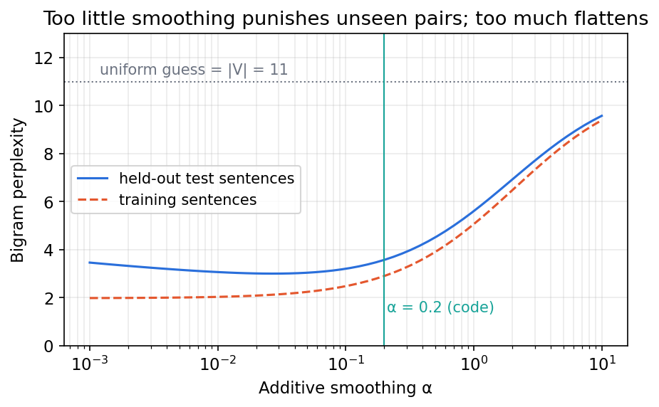
Distinguish smoothing from longer memory
Smoothing addresses missing observations within the chosen representation. It does not restore discarded history. After either “the technician did not repair the” or “the technician repaired the,” a bigram sees only the. It assigns the same next-token distribution even if the earlier words would make different continuations appropriate. Increasing the corpus can estimate that shared distribution more accurately while leaving the equality intact.
Additive smoothing also has an exact mixture interpretation. For a context with a positive observed count:
Here is the smoothed distribution, is the retained history, is a candidate token, is its observed transition count, is the total outgoing count, is the unsmoothed estimate, is the smoothing parameter, is vocabulary size and is the weight on observations. A context with zero count uses the uniform distribution directly.
The same smoothing parameter changes rare contexts more than frequent ones. As context count grows, the observed evidence receives more weight; as smoothing grows, probability moves toward the uniform distribution. This explains why a held-out curve can improve initially and then worsen: protecting unseen transitions eventually also dilutes useful observed distinctions. Choose the parameter with validation data rather than the final test set.
A tokenizer and unknown-token rule are part of this experiment. Mapping several unseen words to one marker pools their probabilities. A lower perplexity after that mapping can partly reflect an easier prediction alphabet. It does not show that the model can identify those original words.
Interpolate evidence from several history lengths
When a long context is rare, shorter contexts often have more observations. Interpolation combines their complete distributions instead of assigning every unseen continuation the same probability.
Here are the two most recent tokens; is the next token; are normalized trigram, bigram and unigram distributions; is their mixture; and is the nonnegative weight assigned to order . Each component must be defined for the queried history, for example by smoothing. Summing over candidate tokens gives one because each component sums to one and the weights also sum to one.
For the unseen context in our small comparison, a mixture can use the observed bigram after cat even though the full two-token context is missing. Fixed mixture weights are easy to inspect; history-dependent weights can assign more trust to well-supported longer histories. Choose the weights on validation text. Deciding them after inspecting the final test perplexity makes that score part of model selection.
Interpolation differs from simply substituting a shorter history only when a transition is missing. Such back-off rules must also account for the probability already allocated to observed transitions, so that the complete distribution stays normalized. Chen and Goodman’s comparative study examines smoothing choices and their empirical behavior [4]. Our additive and mixture examples expose the mechanics rather than implementing every estimator in that study.
4. What held-out perplexity measures
Scoring measures how much probability a model gives the observed targets. A good score means that these particular token sequences were relatively unsurprising under a particular tokenizer and vocabulary; it does not establish factual accuracy or understanding.
Here is the number of scored token positions; indexes those positions across the evaluated sentences; is the observed target; is its permitted history; is the evaluated model; is mean negative log likelihood in nats per token; and is perplexity. The product form shows that perplexity is the geometric mean of reciprocal target probabilities. It is not the count of plausible continuations at every position.
If every observed target receives probability , perplexity equals , where is the number of equally likely choices in that hypothetical distribution. Actual predictions are not uniform: one difficult target can contribute a large log loss while many easy targets contribute little. Reporting only an average can conceal concentrated failure on rare names or unfamiliar domains. Inspect losses by word frequency and sentence type as well.
When aggregating batches, add their total negative log likelihoods and divide by the total number of scored tokens before exponentiating. Neither averaging batch perplexities nor exponentiating an unweighted mean of batch losses generally gives corpus perplexity. The latter is correct only when the batches have equal scored-token counts. Padding and a short final batch make that assumption easy to violate. This synthetic calculation follows directly from the definition above:
Code · Python · 10 lines
import math

# Synthetic evaluation batches: 2 targets of probability 1/2, then 8 of 1/4.
counts = [2, 8]
mean_nll = [math.log(2), math.log(4)]
corpus_ppl = math.exp(sum(n * loss for n, loss in zip(counts, mean_nll)) / sum(counts))
print('token-weighted perplexity:', round(corpus_ppl, 3))
print('mean batch perplexity:', round(sum(math.exp(loss) for loss in mean_nll) / 2, 3))
print('exp of mean batch loss:', round(math.exp(sum(mean_nll) / 2), 3))
assert math.isclose(corpus_ppl, (2**2 * 4**8)**(1 / 10))
Output
token-weighted perplexity: 3.482
mean batch perplexity: 3.0
exp of mean batch loss: 2.828
The bigram code counts the end marker, which makes stopping part of both the training problem and the evaluation. It excludes the beginning marker. Its unigram and bigram results are comparable because the test text, tokenization, unknown mapping and number of scored positions match. A comparison across word and character tokenizers has different units. Even the same raw sentence can yield a different score denominator and prediction alphabet.
Train, validation and test text have separate roles. Training determines vocabulary and counts; validation selects order and smoothing; test evaluates the chosen pipeline once. A held-out spelling absent from training must follow the fixed unknown rule. Rebuilding the vocabulary with test text silently changes the experiment. Repeated sentences or material copied across splits can also make memorized local continuations look like generalization.
5. Generation, stopping and the memory ceiling
Generation repeatedly samples from a normalized next-token distribution, appends the sampled token to the history and stops when the end marker appears. Scoring instead supplies the observed history from the text being evaluated. The same probability tables support both procedures, but one examines supplied text while the other produces a stochastic trajectory.
The demonstrated sample a bird sings is one draw with a fixed random seed. It is not a representative quality estimate. Examine several independently seeded trajectories and report both local errors and unusually long sequences. A length cap guarantees that a program stops running; if the cap fires before the end marker, the displayed sequence is truncated rather than a model-generated completed sentence.
Choosing the most probable next token at each step gives a deterministic greedy trajectory. It does not generally maximize the probability of the entire sequence: a locally attractive token may lead to poor later continuations. Conversely, sampling preserves distributional variety but may choose low-probability transitions. Generation choices therefore answer a different question from whether the model assigns good probabilities to held-out text.
A failure that more training cannot remove
Consider the robot near the cabinets is and the robots near the cabinet are. Agreement depends on the head of the subject, rather than simply the immediately preceding noun. If the relevant head lies outside the retained suffix, the model pools examples that require different agreement choices. More observations can improve the pooled estimate, but cannot make that estimate depend on a token outside the model’s input.
For any two prefixes with the same final tokens, an n-gram model’s next-token distributions must be identical. This is an architectural equality, not an empirical tendency. Increase and the ceiling moves farther away, while the number of possible histories and the sparsity of their count tables increase. Shared neural representations can connect similar contexts, but their actual behavior still requires testing; merely replacing a table does not establish that an agreement dependency was learned.
6. A recurrent language model
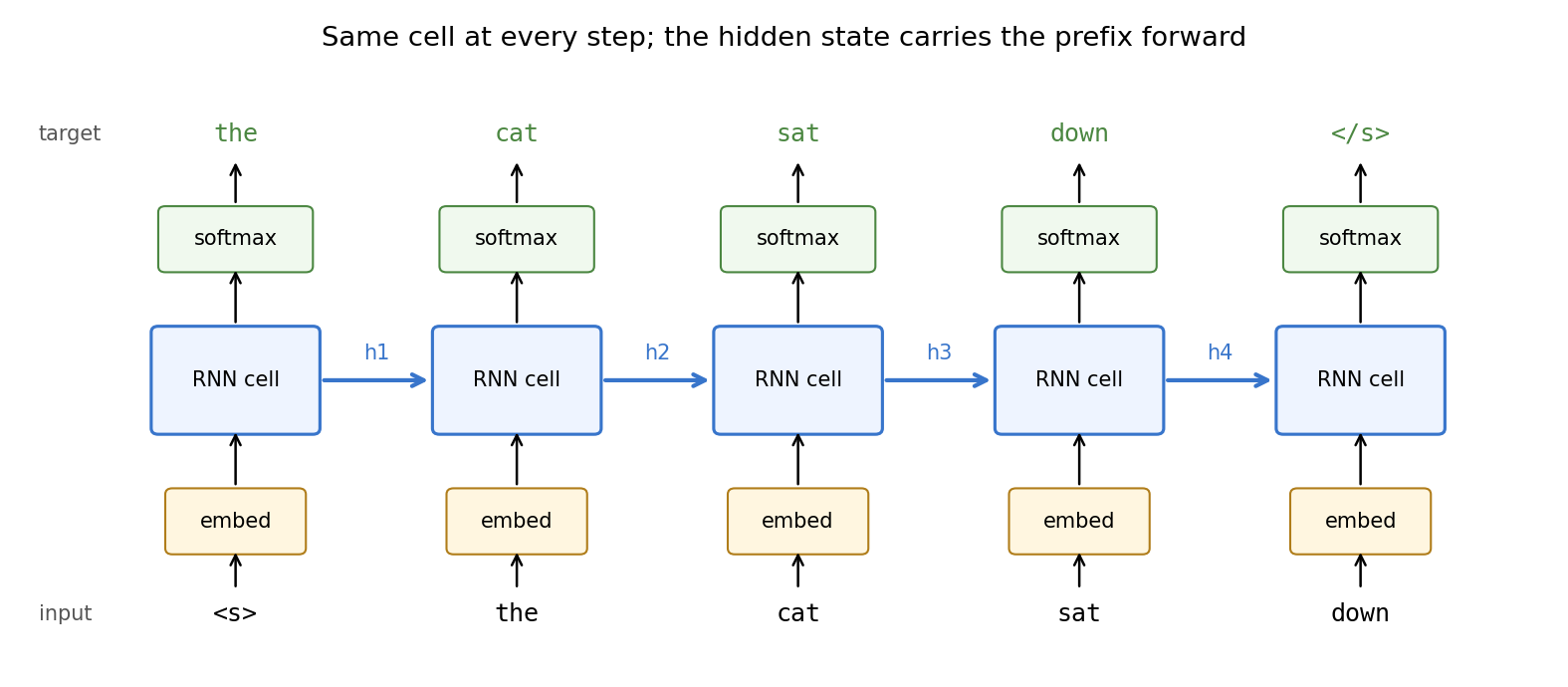
Plain version. An n-gram model looks the history up in a table. A recurrent language model reads the history one token at a time and keeps a fixed-size vector, the hidden state, that it updates after each token. The next-token distribution is computed from that state, so the model is no longer forced to forget everything older than tokens.
Elman’s simple recurrent network introduced this idea of a state fed back as input at the next step [6]; Mikolov and colleagues showed that a recurrent network trained as a word-level language model could beat strong smoothed n-gram baselines for speech recognition [7]. Keep the chain rule from section 2 exactly as it was. Only the conditional distribution changes. For a token sequence with a beginning marker :
Here is the embedding of token (a row of a learned table, as in NLP 04); is the hidden state after reading ; , and are the recurrent parameters; and map the state to one score per vocabulary item ; is the prediction vocabulary and ranges over it; collects all parameters; and acts element by element. This is the same recurrence as in ML 03A, written with an embedding as input and a softmax over the vocabulary as output.
Three consequences follow directly from the equations.
- Unbounded conditioning, bounded memory. is a function of the whole prefix, so two prefixes that share their last tokens can receive different predictions. But has only numbers. The model must learn what to keep; nothing guarantees that it keeps the information a particular dependency needs.
- Shared parameters. The same , and are used at every position. The parameter count does not grow with context length, whereas the number of possible n-gram histories grows as .
- Generalization through similarity. Similar tokens receive similar embeddings, and similar prefixes can produce similar states. An unseen history no longer falls back to a uniform row: it is mapped to some state, and the prediction made from that state can reuse what similar histories taught the model.
The training loss is next-token cross-entropy
Training minimizes the same quantity that section 4 used for evaluation, now as a differentiable function of :
Here is the number of supervised target positions (padding and other ignored positions excluded), is the observed target at position , is its prefix, and converts nats to bits. The per-position term is the cross-entropy between the one-hot target and the model’s softmax distribution; IT 01 develops cross-entropy and its link to coding length. Character-level work often reports bits per character instead of perplexity; the two carry the same information.
Two implementation details carry over from the count model. First, shift by one: the input sequence is and the target sequence is . Feeding a position’s own token as both input and target creates a trivial copying shortcut. Second, teacher forcing: during training each step receives the observed previous token, not the model’s own earlier sample. At generation time, the model’s samples become its inputs, so errors can feed on themselves. Training loss and sampling behavior therefore need separate checks, exactly as section 5 argued for the n-gram model.
7. Training through time: what gradients can reach
Plain version. Unrolling the recurrence turns the model into a very deep network with tied weights. Gradients from a prediction must travel back through every intermediate step to reach the token that should have influenced it. Over long distances they tend to shrink to almost nothing or, less often, blow up.
Backpropagation through time (BPTT) applies ordinary backpropagation to the unrolled graph and sums the gradient contributions for each shared weight [8]. The sensitivity of a later state to an earlier one is an ordered product of one-step Jacobians:
where are positions, squares each element, and builds a diagonal matrix from the derivatives. When the factors are typically smaller than one in norm, the product decays exponentially with distance (vanishing gradients); when they are larger, it can grow exponentially (exploding gradients). Bengio, Simard and Frasconi analyzed why learning long-term dependencies with gradient descent is hard [9]; Pascanu, Mikolov and Bengio revisited the problem and popularized clipping the gradient norm as the remedy for explosions [10]. ML 03A derives these results in full and measures them.
What does this mean for language? Return to the agreement example from section 5: in the robots near the cabinet are, the verb depends on robots, four words back, and the intervening noun points the other way. A plain RNN can represent a state that remembers the plural subject, but the training signal that would teach it to do so must survive the trip from are back to robots. At the word level that is a few steps; at the character level the same dependency spans roughly twenty steps. A model can therefore have enough capacity for a dependency and still fail to learn it, which is a different failure from the n-gram’s architectural ceiling.
8. Gated cells: LSTM and GRU
Plain version. Gated cells add a memory path that is updated mainly by addition and controlled by learned switches. Information, and gradient, can then pass across many steps without being squashed at every one.
The long short-term memory (LSTM) cell of Hochreiter and Schmidhuber [11], with the forget gate added by Gers, Schmidhuber and Cummins [12], keeps a cell state next to the hidden state:
Here , and are the forget, input and output gates (vectors in computed by sigmoid layers from the current input and ), is a candidate computed the same way, and is element-wise multiplication. Along the cell path, is approximately : no weight matrix, no squashing. When a forget gate stays near one, a value written at the plural subject can survive until the verb.
The gated recurrent unit (GRU) of Cho and colleagues [13] merges cell and hidden state and uses two gates:
where is the update gate and is a candidate state computed with a reset gate. (Some sources swap the roles of and .) The full gate equations, a from-scratch LSTM step checked against PyTorch, and parameter counts are in ML 03A. For language modeling the practical summary is: LSTMs and GRUs train far more reliably than plain RNNs, neither dominates the other across tasks, and gating eases rather than removes the difficulty of very long dependencies.
9. Stacked and bidirectional recurrent networks
Plain version. Recurrent layers can be stacked so that a higher layer reads the state sequence of the layer below. Running a second network right to left gives each position a view of its future too, which is useful for labeling text but forbidden for predicting the next token.
A stacked (deep) RNN feeds from layer as the input sequence of layer , and the softmax reads the top layer. Two to four layers are common in recurrent language models; dropout between layers is the usual regularizer [16].
A bidirectional RNN runs one network forward and one backward and concatenates their states, [14]. The backward state at position has read . That is ideal for tagging, where the whole sentence is given and the label of a word may depend on words to its right; it is the main encoder of NLP 06. It is wrong for a left-to-right language model: if the state used to predict has seen , the loss rewards copying and the perplexity becomes meaningless. A useful sanity check for any language model is that changing a future token leaves every earlier prediction unchanged.
Optional: Seq2Seq (in the Paper guides). Follow the original figure, objective, experimental comparisons and limitations.
10. Character-level language models
Plain version. The prediction unit can be a character instead of a word. The vocabulary becomes tiny and no spelling is ever unknown, but sequences become several times longer and the model must learn spelling before it can learn grammar.
Character-level RNNs were popular demonstrations of what recurrent networks learn; Graves showed that LSTMs trained on characters can generate long, locally coherent text and handwriting [15]. The tradeoffs compared with word or subword units are concrete:
| Choice | Vocabulary | Unknown inputs | Sequence length | Long-range cost |
|---|---|---|---|---|
| Words | Large; rare words need an unknown marker | Mapped to one marker; spelling lost | Shortest | Fewest steps between related words |
| Subwords (NLP 01) | Medium, fixed by the tokenizer | Split into known pieces | Medium | Medium |
| Characters | Tiny alphabet | Any spelling over the alphabet | Longest | Many steps between related words |
Two cautions follow from the evaluation rules in section 4. First, character perplexity and word perplexity have different units; a character model with perplexity 11 is not “better” than a word model with perplexity 3.6, because each counts a different number of predictions over a different alphabet. For a comparison using a common text unit, report total negative log likelihood (or bits) for the same text and, if needed, divide by a common byte count. This requires compatible, lossless text preprocessing and declared boundary conventions: replacing unknown spellings with one marker does not encode the missing characters. A change of denominator cannot repair information erased before scoring. Second, a fixed character alphabet still needs a policy for symbols outside it, such as accented letters or emoji. Decide it before looking at held-out text.
11. Sampling and temperature
Plain version. A trained model gives a probability for every next token. To generate, we draw one, append it, and repeat. A temperature setting makes the draw more cautious or more adventurous without retraining.
For logits and temperature , sample from
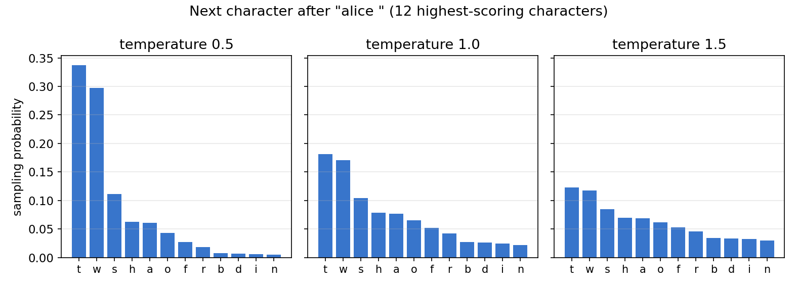
Here and range over the vocabulary , is the model’s score for at step , and is the sampling distribution. samples from the model’s own distribution; approaches greedy selection of the highest-scoring token; flattens the distribution and gives more weight to unlikely tokens. Temperature changes only the generation procedure. It does not change the probabilities used to compute perplexity, so a model’s held-out score is the same at every temperature.
Generation adds stopping rules, length limits and search strategies such as beam search and nucleus sampling. Those belong to NLP 08 and NLP 09. One warning applies already: a sample is a single random trajectory. Judge a model by held-out likelihood and task checks, and use samples to look for qualitative failure patterns, not to rank models.
12. Practical training, then a complete experiment
The training checklist
Plain version. Most failed recurrent language models fail for mundane reasons: padding counted as text, gradients that explode, states leaking between unrelated documents, or a model selected on the test set. Each has a standard remedy.
- Packing a corpus into streams. For a continuous text, cut the token stream into equal parallel streams and lay them out as a matrix. Each training step reads the next columns. Every position is a real token, so no padding is needed. Stream continues exactly where it stopped in the previous window.
- Padding and masking. When examples are separate sentences of different lengths, pad them to a common length and keep a Boolean mask. The mask must remove padded positions from the loss (otherwise the model is rewarded for predicting padding) and, for bidirectional encoders, from the state updates; PyTorch’s
pack_padded_sequencedoes the latter. NLP 06 implements both in a tagger. - Truncated BPTT. Backpropagating through thousands of steps costs memory linear in the length. Instead, carry the hidden state from one window of steps to the next but detach it, so the forward pass still sees the whole past while gradients flow back at most steps.
- Gradient clipping. If the gradient norm exceeds a threshold , rescale it to [10]. This keeps the update direction and caps its length.
- Regularization and early stopping. Dropout on non-recurrent connections [16] and weight decay limit memorization; select the epoch with the lowest validation perplexity, then report test perplexity once.
- Fair baselines. Melis, Dyer and Blunsom found that carefully tuned standard LSTMs outperformed several more elaborate recent architectures once all were given comparable hyperparameter search [17]. The same principle applies at small scale: tune the n-gram baseline on the same validation data before claiming that the neural model wins.
Code: a character-level LSTM against an interpolated n-gram
The text is the opening of Chapter I of Lewis Carroll’s Alice’s Adventures in Wonderland (1865), which is in the public domain; it was copied from Project Gutenberg eBook #11 [24] with italic underscores removed, curly quotes straightened and em dashes written as --, then lowercased. Paragraphs 1–7 are training data, paragraph 8 is validation and paragraph 9 is the test set. The alphabet is fixed in advance, before the held-out text is inspected. Both models condition each held-out character on all earlier text. The n-gram baseline interpolates smoothed unigram, bigram and trigram character distributions exactly as in section 3, with weights and smoothing chosen on validation. The LSTM is trained three times with different seeds, because a single run on so little data can mislead. The whole script runs on a CPU in well under a minute and downloads nothing.
Code · Python · 215 lines
import copy
import math
from collections import Counter, defaultdict

import torch
from torch import nn

# Opening paragraphs of Chapter I of Lewis Carroll's "Alice's Adventures in
# Wonderland" (1865, public domain; Project Gutenberg eBook #11). Italic
# underscores removed, curly quotes straightened, em dashes written as "--".
PARAGRAPHS = [
    'Alice was beginning to get very tired of sitting by her sister on the '
    'bank, and of having nothing to do: once or twice she had peeped into the '
    'book her sister was reading, but it had no pictures or conversations in '
    'it, "and what is the use of a book," thought Alice "without pictures or '
    'conversations?"',
    'So she was considering in her own mind (as well as she could, for the hot '
    'day made her feel very sleepy and stupid), whether the pleasure of making '
    'a daisy-chain would be worth the trouble of getting up and picking the '
    'daisies, when suddenly a White Rabbit with pink eyes ran close by her.',
    'There was nothing so very remarkable in that; nor did Alice think it so '
    'very much out of the way to hear the Rabbit say to itself, "Oh dear! Oh '
    'dear! I shall be late!" (when she thought it over afterwards, it occurred '
    'to her that she ought to have wondered at this, but at the time it all '
    'seemed quite natural); but when the Rabbit actually took a watch out of '
    'its waistcoat-pocket, and looked at it, and then hurried on, Alice started'
    ' to her feet, for it flashed across her mind that she had never before '
    'seen a rabbit with either a waistcoat-pocket, or a watch to take out of '
    'it, and burning with curiosity, she ran across the field after it, and '
    'fortunately was just in time to see it pop down a large rabbit-hole under '
    'the hedge.',
    'In another moment down went Alice after it, never once considering how in '
    'the world she was to get out again.',
    'The rabbit-hole went straight on like a tunnel for some way, and then '
    'dipped suddenly down, so suddenly that Alice had not a moment to think '
    'about stopping herself before she found herself falling down a very deep '
    'well.',
    'Either the well was very deep, or she fell very slowly, for she had plenty'
    ' of time as she went down to look about her and to wonder what was going '
    'to happen next. First, she tried to look down and make out what she was '
    'coming to, but it was too dark to see anything; then she looked at the '
    'sides of the well, and noticed that they were filled with cupboards and '
    'book-shelves; here and there she saw maps and pictures hung upon pegs. She'
    ' took down a jar from one of the shelves as she passed; it was labelled '
    '"ORANGE MARMALADE", but to her great disappointment it was empty: she did '
    'not like to drop the jar for fear of killing somebody underneath, so '
    'managed to put it into one of the cupboards as she fell past it.',
    '"Well!" thought Alice to herself, "after such a fall as this, I shall '
    "think nothing of tumbling down stairs! How brave they'll all think me at "
    "home! Why, I wouldn't say anything about it, even if I fell off the top of"
    ' the house!" (Which was very likely true.)',
    'Down, down, down. Would the fall never come to an end? "I wonder how many '
    'miles I\'ve fallen by this time?" she said aloud. "I must be getting '
    'somewhere near the centre of the earth. Let me see: that would be four '
    'thousand miles down, I think--" (for, you see, Alice had learnt several '
    'things of this sort in her lessons in the schoolroom, and though this was '
    'not a very good opportunity for showing off her knowledge, as there was no'
    ' one to listen to her, still it was good practice to say it over) "--yes, '
    "that's about the right distance--but then I wonder what Latitude or "
    'Longitude I\'ve got to?" (Alice had no idea what Latitude was, or Longitude'
    ' either, but thought they were nice grand words to say.)',
    'Presently she began again. "I wonder if I shall fall right through the '
    "earth! How funny it'll seem to come out among the people that walk with "
    'their heads downward! The Antipathies, I think--" (she was rather glad '
    "there was no one listening, this time, as it didn't sound at all the right"
    ' word) "--but I shall have to ask them what the name of the country is, '
    'you know. Please, Ma\'am, is this New Zealand or Australia?" (and she tried'
    " to curtsey as she spoke--fancy curtseying as you're falling through the "
    'air! Do you think you could manage it?) "And what an ignorant little girl '
    "she'll think me for asking! No, it'll never do to ask: perhaps I shall see"
    ' it written up somewhere."',
]

paras = [p.lower() for p in PARAGRAPHS]
train = "\n".join(paras[:7]) + "\n"     # paragraphs 1-7: fit parameters
valid = paras[7] + "\n"                 # paragraph 8: choose settings
test = paras[8] + "\n"                  # paragraph 9: report once
ALPHABET = "\n !\"'(),-.:;?abcdefghijklmnopqrstuvwxyz"  # fixed in advance
V = len(ALPHABET)
assert set(train + valid + test) <= set(ALPHABET)
print("characters train/valid/test:", len(train), len(valid), len(test))
print("letters never seen in training:", sorted(set(valid + test) - set(train)))

# ---- Baseline: interpolated character n-grams (orders 1-3) ----
def count(order):
    rows = defaultdict(Counter)
    for t in range(len(train)):
        rows[train[max(0, t - order + 1):t]][train[t]] += 1
    return rows

tables = {k: count(k) for k in (1, 2, 3)}

def p_add(k, history, ch, alpha):
    row = tables[k].get(history[len(history) - k + 1:] if k > 1 else "", {})
    return (row.get(ch, 0) + alpha) / (sum(row.values()) + alpha * V)

def ngram_ppl(prefix, target, lams, alpha):
    full, nll = prefix + target, 0.0
    for pos in range(len(prefix), len(full)):
        h = full[max(0, pos - 2):pos]
        p = sum(l * p_add(k, h, full[pos], alpha) for k, l in zip((1, 2, 3), lams))
        nll -= math.log(p)
    return math.exp(nll / len(target))

grid = [(l1, l2, round(1 - l1 - l2, 2)) for l1 in (0.1, 0.2, 0.3)
        for l2 in (0.2, 0.3, 0.4, 0.5) if l1 + l2 < 1]
best_cfg = min(((ngram_ppl(train, valid, lams, a), lams, a) for lams in grid
                for a in (0.01, 0.1, 0.5)), key=lambda r: r[0])
ng_valid, ng_lams, ng_alpha = best_cfg
ng_test = ngram_ppl(train + valid, test, ng_lams, ng_alpha)
print(f"n-gram  weights={ng_lams} alpha={ng_alpha}  "
      f"valid PPL={ng_valid:.2f}  test PPL={ng_test:.2f}")

tri_alpha = min((0.01, 0.1, 0.5), key=lambda a: ngram_ppl(train, valid, (0, 0, 1), a))
tri_test = ngram_ppl(train + valid, test, (0, 0, 1), tri_alpha)
print(f"trigram only  alpha={tri_alpha}  test PPL={tri_test:.2f}")

# ---- Character-level LSTM language model ----
stoi = {c: i for i, c in enumerate(ALPHABET)}
encode = lambda s: torch.tensor([stoi[c] for c in s])

class CharLSTM(nn.Module):
    def __init__(self, vocab, emb=24, hidden=96, dropout=0.3):
        super().__init__()
        self.emb = nn.Embedding(vocab, emb)
        self.rnn = nn.LSTM(emb, hidden, batch_first=True)
        self.drop = nn.Dropout(dropout)
        self.out = nn.Linear(hidden, vocab)

    def forward(self, x, state=None):
        h, state = self.rnn(self.emb(x), state)
        return self.out(self.drop(h)), state

def lstm_ppl(model, prefix, target):
    model.eval()
    with torch.no_grad():
        ids = encode(prefix + target).unsqueeze(0)
        logits, _ = model(ids[:, :-1])          # condition on all earlier text
        nll = nn.functional.cross_entropy(logits[0, len(prefix) - 1:],
                                          ids[0, len(prefix):])
    model.train()
    return math.exp(nll.item())

def train_lstm(seed, epochs=80, B=16, T=48):
    torch.manual_seed(seed)
    model = CharLSTM(V)
    opt = torch.optim.Adam(model.parameters(), lr=3e-3, weight_decay=1e-4)
    ids = encode(train)
    n = (len(ids) - 1) // B                     # B parallel streams of n characters
    X, Y = ids[:n * B].view(B, n), ids[1:n * B + 1].view(B, n)  # targets shifted by one
    history, best = [], (float("inf"), None, 0)
    for epoch in range(1, epochs + 1):
        state, total, steps = None, 0.0, 0
        for i in range(0, n, T):
            if state is not None:               # truncated BPTT: keep values, cut graph
                state = tuple(s.detach() for s in state)
            logits, state = model(X[:, i:i + T], state)
            loss = nn.functional.cross_entropy(logits.reshape(-1, V),
                                               Y[:, i:i + T].reshape(-1))
            opt.zero_grad()
            loss.backward()
            nn.utils.clip_grad_norm_(model.parameters(), 1.0)
            opt.step()
            total, steps = total + loss.item(), steps + 1
        v = lstm_ppl(model, train, valid)
        history.append((epoch, math.exp(total / steps), v))
        if v < best[0]:                         # early stopping on validation only
            best = (v, copy.deepcopy(model.state_dict()), epoch)
    model.load_state_dict(best[1])
    return model, best, history

runs = {}
for seed in (0, 1, 2):
    m, best, hist = train_lstm(seed)
    runs[seed] = (m, hist, lstm_ppl(m, train + valid, test))
    print(f"LSTM seed={seed}  best epoch={best[2]}  valid PPL={best[0]:.2f}  "
          f"test PPL={runs[seed][2]:.2f}")
mean_test = sum(r[2] for r in runs.values()) / len(runs)
print(f"LSTM mean test PPL over 3 seeds: {mean_test:.2f}")
assert mean_test < tri_test
model = runs[0][0]

# ---- Sampling at several temperatures ----
def sample(prompt, tau, length=80, seed=1):
    g = torch.Generator().manual_seed(seed)
    model.eval()
    with torch.no_grad():
        logits, state = model(encode(prompt).unsqueeze(0))
        out = prompt
        for _ in range(length):
            probs = torch.softmax(logits[0, -1] / tau, dim=-1)
            nxt = torch.multinomial(probs, 1, generator=g)
            out += ALPHABET[nxt.item()]
            logits, state = model(nxt.view(1, 1), state)
    return out.replace("\n", " / ")

for tau in (0.5, 1.0, 1.5):
    print(f"tau={tau}:", sample("alice ", tau))

# ---- Same last two characters, different earlier context ----
def next_dist(prefix):
    model.eval()
    with torch.no_grad():
        logits, _ = model(encode(prefix).unsqueeze(0))
    return torch.softmax(logits[0, -1], dim=-1)

a, b = "alice was beginning to get ", "the rabbit-hole went "
assert a[-2:] == b[-2:]                     # a trigram sees only these two
def ngram_dist(prefix):
    return torch.tensor([sum(l * p_add(k, prefix[-2:], c, ng_alpha)
                             for k, l in zip((1, 2, 3), ng_lams)) for c in ALPHABET])

tv = lambda p, q: 0.5 * (p - q).abs().sum().item()
print("total variation, n-gram:", round(tv(ngram_dist(a), ngram_dist(b)), 3),
      " LSTM:", round(tv(next_dist(a), next_dist(b)), 3))
Output:
Code · 12 lines
characters train/valid/test: 2633 706 682
letters never seen in training: ['z']
n-gram  weights=(0.1, 0.4, 0.5) alpha=0.01  valid PPL=9.70  test PPL=11.24
trigram only  alpha=0.1  test PPL=13.37
LSTM seed=0  best epoch=43  valid PPL=10.13  test PPL=12.09
LSTM seed=1  best epoch=41  valid PPL=9.76  test PPL=11.05
LSTM seed=2  best epoch=39  valid PPL=10.09  test PPL=11.30
LSTM mean test PPL over 3 seeds: 11.48
tau=0.5: alice whas she sor of the to her fear the she was she sely and it she save of the was
tau=1.0: alice whas nyt ook "hente tome urabuint, mubbeit-insiwselly bulith ver to welf was bor
tau=1.5: alice wherany fowh ".pvenst gime feurdt, )ubger and iwselly ?hont  ver, vermef wamen r
total variation, n-gram: 0.0  LSTM: 0.197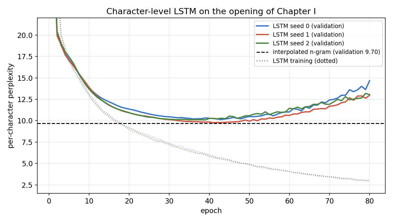
Reading the results
The baseline matters. A single trigram with additive smoothing reaches a test perplexity of 13.37, and every LSTM run beats it. The interpolated n-gram, tuned on the same validation paragraph, reaches 11.24, while the three LSTM runs reach 12.09, 11.05 and 11.30 (mean 11.48). On 2,633 training characters the recurrent model is roughly level with a well-smoothed count model and clearly better than a poorly smoothed one. This is the small-data version of the point made by Melis and colleagues [17]: an improvement claimed against an untuned baseline may vanish against a tuned one. Neural language models pull ahead as data grows, because shared representations can exploit many weak regularities that sparse tables cannot pool; Jozefowicz and colleagues document how far recurrent language models improved with large corpora and models [19]. Our experiment is far too small to show that regime, and it does not need to: it shows how to make the comparison honestly.
Seeds matter. The spread across seeds (11.05 to 12.09) is larger than the gap between the mean LSTM and the n-gram. With one seed, we could have reported either “the LSTM wins” or “the LSTM loses”. Report several runs, or a confidence interval over held-out documents, whenever differences are this small.
The validation curve shows memorization. In Figure 4, training perplexity keeps falling far below the validation value. The model is learning the specific training paragraphs. Early stopping picks epochs 39–43; without it, the final epoch would be considerably worse on held-out text.
Units. These are per-character perplexities over a 39-symbol alphabet; bits per character for the n-gram. They cannot be compared with the word-level values of section 3 (for example 3.573), which count different events over a different vocabulary.
The memory ceiling, measured. The final lines compare next-character distributions after alice was beginning to get and the rabbit-hole went , two prefixes whose last two characters agree. The interpolated trigram must give identical distributions (total variation 0.0), exactly as section 5 proved. The LSTM’s distributions differ (total variation 0.197), because its state depends on the earlier characters. This confirms that the recurrent model uses longer context. Whether it uses it well is a separate question, which held-out perplexity and targeted tests answer.
Samples. At the sample repeats frequent fragments such as she was and of the; at word shapes appear with many misspellings; at the output breaks into rare punctuation and random letters. A character model trained on fewer than three thousand characters has learned frequent letter sequences, spaces and some short words. It has not learned English. These are single draws with one seed, so read them as illustrations of the temperature effect rather than as quality estimates.
Modern view
Survey perspective. Jurafsky and Martin’s August 2026 draft retains a dedicated n-gram chapter, organized around probabilistic prediction, estimation, evaluation, generation and smoothing [3]. It is a useful conceptual bridge: readers can inspect local counts before encountering models that share learned representations. Chen and Goodman’s smoothing comparison explains why the estimator matters in addition to the history length [4]. These sources serve different purposes: the textbook develops the model, while the empirical study compares ways to allocate probability with sparse evidence. Tiezzi and colleagues’ 2024 survey reviews why recurrent processing has returned in the Transformer era [20]. It frames two trends under one umbrella of recurrence: models that mix Transformer and recurrent ideas to avoid the quadratic cost of self-attention, and deep state-space models that act as a special class of linear RNNs. Its main open problem is learning from streams whose length is not known in advance, which connects sequence modeling to lifelong online learning.
What recurrent language models achieved. From Mikolov’s RNN language model [7] to large-scale LSTM language models [19] and carefully regularized LSTMs [18], recurrent networks were the strongest general-purpose language models until Transformers replaced them for most large-scale work. Merity and colleagues’ AWD-LSTM study shows how much of that strength came from regularization and optimization choices rather than from new cell designs [18]; Melis and colleagues reached a similar conclusion through controlled hyperparameter search [17].
2023–2026. Recurrence has returned in new forms aimed at the cost of attention over long contexts. RWKV reformulates a Transformer-like model so it can be trained in parallel and run as an RNN at inference [21]. Mamba uses input-dependent (selective) state-space updates computed with a parallel scan [22]. xLSTM revisits the LSTM with exponential gating and new memory structures [23]. These models keep the property that made RNN language models attractive: a fixed-size state, so generation cost per token does not grow with context length. They also inherit the question raised in section 7: a fixed-size state must decide what to forget. ML 03A covers the state-space side in more detail.
Evaluation. Chang and colleagues’ 2024 survey organizes large-language-model evaluation around what, where and how to evaluate [5]. It covers task behavior and evaluation methods beyond token prediction. Applied here, a lower perplexity should be accompanied by the task checks that matter: spelling recovery, agreement, meaning preservation or an appropriate stopping rule. The practical role of an n-gram baseline in a 2023–2026 workflow is to make a question measurable. Does a more elaborate model improve held-out predictions under the same tokenization? Does it distinguish two prefixes that the chosen n-gram history must merge? Does its added memory and latency improve the downstream result? Answer with matched experiments rather than comparing unmatched scores or assuming that a longer context is always used effectively.
Open problems. Open problems include sparse evidence after domain changes, probabilities for new names, and interactions between tokenization and measured difficulty. Character or subword tokens change the tradeoff between vocabulary coverage and sequence length. Longer histories, whether held in a table or in a recurrent state, offer more information but create harder estimation and credit-assignment problems. Choose the prediction unit and retained history together, and state their limits before interpreting a result.
Key takeaways
- An n-gram occurrence or document feature is not automatically a normalized language model; order uses preceding tokens, while the chain rule itself does not require limited memory.
- Smoothing protects unobserved events, and interpolation reuses shorter-history evidence; neither can recover history that the model discarded.
- Perplexity comparisons need matching prediction units, unknown mapping and boundary conventions; character and word perplexities are not comparable.
- A recurrent language model replaces the count table with a learned state that depends on the whole prefix, with parameters shared across positions.
- BPTT gradients shrink or grow with distance; clipping handles explosions, and LSTM or GRU gating eases vanishing gradients without removing the difficulty of long dependencies.
- Bidirectional RNNs suit labeling, not left-to-right language modeling.
- Practical training needs shifted targets, masks or packed streams, truncated BPTT, clipping, regularization and validation-based early stopping.
- On tiny data, a tuned interpolated n-gram can match an LSTM; compare against tuned baselines and report several seeds.
Exercises
- Reproduce the smoothed trigram probabilities after
a catandthe catby hand in the first code example of section 2. Check the sum over all eight target tokens.
Hint
Each history has one observation. The denominator is one plus the smoothing strength multiplied by eight; only the observed continuation receives an additional count.
- Fit a mixture of the first example’s three orders. Choose any nonnegative weights summing to one, and verify normalization for an unseen two-token history.
Hint
Evaluate every component on the same candidate vocabulary. Compare the probability after the unseen history with the pure uniform fallback and the observed bigram after cat.
- Score the bigram test set both including and excluding end markers. Explain why the resulting perplexities answer different prediction questions.
Hint
Change both the accumulated loss and the position count consistently. Excluding end markers removes the evaluation of stopping; it is not merely changing a display convention.
- Construct two prefixes with identical last two tokens whose appropriate next-token probabilities should differ because of earlier negation, agreement or discourse. State what a trigram can and cannot learn about them, and what an RNN language model could learn about them in principle.
Hint
First confirm that the retained history is exactly equal. Then separate a lack of data from the impossibility of conditioning on the omitted distinction. For the RNN, distinguish what its state can represent from what its gradients can teach it.
- In the character-level experiment, replace
nn.LSTMwithnn.GRU(the state becomes a single tensor, so adjust the detach line) and withnn.RNN. Compare validation and test perplexity over three seeds. Then remove gradient clipping from the plain RNN and record what happens to the training loss.
Hint
nn.GRU and nn.RNN return a tensor rather than a tuple as their state. Keep every other setting fixed, including the early-stopping rule, so that the cell type is the only change.
- Deliberately break causality: give the LSTM model an extra backward LSTM over the same input (a bidirectional layer) and retrain. Explain the training and validation perplexities you observe, and write a test that would have caught the bug.
Hint
With a backward pass, the state used to predict the character at position has already read that character. A good test changes one future character and checks that all earlier predicted distributions are unchanged.
References
- Masato Hagiwara, Real-World Natural Language Processing: Practical Applications with Deep Learning, Chapter 5, Manning, 2021. Publisher
- Susan McRoy, Principles of Natural Language Processing, 2021. Chapter
- Daniel Jurafsky and James H. Martin, Speech and Language Processing, third-edition draft, Chapter 3, August 19, 2026. Chapter
- Stanley F. Chen and Joshua Goodman, “An Empirical Study of Smoothing Techniques for Language Modeling,” ACL, 1996. Paper
- Yupeng Chang et al., “A Survey on Evaluation of Large Language Models,” ACM Transactions on Intelligent Systems and Technology, 2024. Paper
- Jeffrey L. Elman, “Finding Structure in Time,” Cognitive Science 14(2), 1990. DOI
- Tomáš Mikolov, Martin Karafiát, Lukáš Burget, Jan Černocký and Sanjeev Khudanpur, “Recurrent Neural Network Based Language Model,” Interspeech, 2010. DOI
- Paul J. Werbos, “Backpropagation Through Time: What It Does and How to Do It,” Proceedings of the IEEE 78(10), 1990. DOI
- Yoshua Bengio, Patrice Simard and Paolo Frasconi, “Learning Long-Term Dependencies with Gradient Descent Is Difficult,” IEEE Transactions on Neural Networks 5(2), 1994. DOI
- Razvan Pascanu, Tomas Mikolov and Yoshua Bengio, “On the Difficulty of Training Recurrent Neural Networks,” ICML, 2013. arXiv
- Sepp Hochreiter and Jürgen Schmidhuber, “Long Short-Term Memory,” Neural Computation 9(8), 1997. DOI
- Felix A. Gers, Jürgen Schmidhuber and Fred Cummins, “Learning to Forget: Continual Prediction with LSTM,” Neural Computation 12(10), 2000. DOI
- Kyunghyun Cho et al., “Learning Phrase Representations using RNN Encoder–Decoder for Statistical Machine Translation,” EMNLP, 2014. arXiv
- Mike Schuster and Kuldip K. Paliwal, “Bidirectional Recurrent Neural Networks,” IEEE Transactions on Signal Processing 45(11), 1997. DOI
- Alex Graves, “Generating Sequences With Recurrent Neural Networks,” arXiv:1308.0850, 2013. arXiv
- Wojciech Zaremba, Ilya Sutskever and Oriol Vinyals, “Recurrent Neural Network Regularization,” arXiv:1409.2329, 2014. arXiv
- Gábor Melis, Chris Dyer and Phil Blunsom, “On the State of the Art of Evaluation in Neural Language Models,” arXiv:1707.05589, 2017. arXiv
- Stephen Merity, Nitish Shirish Keskar and Richard Socher, “Regularizing and Optimizing LSTM Language Models,” arXiv:1708.02182, 2017. arXiv
- Rafal Jozefowicz, Oriol Vinyals, Mike Schuster, Noam Shazeer and Yonghui Wu, “Exploring the Limits of Language Modeling,” arXiv:1602.02410, 2016. arXiv
- Matteo Tiezzi, Michele Casoni, Alessandro Betti, Tommaso Guidi, Marco Gori and Stefano Melacci, “On the Resurgence of Recurrent Models for Long Sequences: Survey and Research Opportunities in the Transformer Era,” arXiv:2402.08132, 2024. arXiv
- Bo Peng et al., “RWKV: Reinventing RNNs for the Transformer Era,” Findings of EMNLP, 2023. Paper
- Albert Gu and Tri Dao, “Mamba: Linear-Time Sequence Modeling with Selective State Spaces,” COLM, 2024. arXiv
- Maximilian Beck et al., “xLSTM: Extended Long Short-Term Memory,” NeurIPS, 2024. Paper
- Lewis Carroll, Alice’s Adventures in Wonderland, 1865; Project Gutenberg eBook #11. Project Gutenberg
- Ilya Sutskever, Oriol Vinyals and Quoc V. Le, “Sequence to Sequence Learning with Neural Networks,” NeurIPS, 2014. Paper
Check your understanding
This tutorial has 6 exercises. Can you solve them without opening the hints?
Go to the exercises ↑Next NLP 06 · Sequence Labeling with RNNs (POS Tagging, Information Extraction) · 35 min