NLP 09 · Language Modeling with Transformers (Natural Language Generation)
Needs: NLP 08 · Sequence-to-Sequence Models with Transformers (Machine Translation, Chatbots)
Navigate: this page and this track: Navigate: this page and this track
On this page
- What you’ll learn1 min
- The big picture2 min
- 1. Causal sequence probability2 min
- 2. Decoder-only Transformer language models2 min
- 3. A runnable causal model2 min
- 4. Training objective and scaling1 min
- 5. Perplexity and meaningful comparison2 min
- 6. Decoding: from a distribution to a text5 min
- 7. Natural language generation tasks6 min
- 8. Evaluating generated text2 min
- 9. Retrieval: finding the evidence to generate from12 min
- 10. Hallucination and retrieval-augmented generation4 min
- 11. Adapting a pretrained generator2 min
- 12. Training practices meet serving constraints2 min
- Modern view2 min
- Key takeaways1 min
- Exercises2 min
- Paper guides
- References
Natural Language Processing
Explore this chapter 2 interactive experiments
Follow fixed logits through temperature scaling, top-k truncation, nucleus truncation and renormalization.
What you’ll learn
- Factor a sequence probability into causal next-token predictions, and train a tiny decoder-only Transformer that obeys that factorization.
- Place the GPT line of models, their training objective and scaling studies in one consistent picture.
- Decode with greedy search, beam search, temperature, top-k and nucleus sampling, and explain what each does and does not change.
- Build and evaluate three generation tasks: extractive and abstractive summarization, data-to-text and open-ended story writing.
- Measure generation with perplexity, ROUGE, human review and model-based judges, knowing the blind spots of each.
- Retrieve evidence with lexical and dense methods and evaluate the ranking with Recall@k, MRR and nDCG.
- Explain hallucination, retrieval-augmented generation and the boundary between retrieved evidence and application instructions.
The big picture
A language model assigns probabilities to text under a specified context. That simple definition connects spelling completion, sentence generation and reusable contextual representations, but these uses do not share the same output contract. Predicting a likely continuation is different from verifying a factual answer. A fluent continuation may reflect common text patterns while being unsuitable for a particular task.
A language application must also choose what to say, express it clearly, and support what it says. These are separate responsibilities. A readable sentence can describe the wrong event; a correct sentence can omit the warning that the user needed. Deploying the generator adds a further responsibility: the result must arrive predictably, with enough recorded context to investigate a failure.
Hagiwara develops language modeling in Chapter 5, attention and Transformers in Chapter 8, pretrained-model adaptation in Chapter 9, and training practice and deployment in Chapters 10–11 [1]. McRoy’s Chapter 6 emphasizes language-model evaluation through tasks, and Chapter 9 develops generation and summarization [2]. This chapter connects the probability model to those practical concerns. We train only tiny synthetic models; large pretrained systems are discussed through verified primary papers and surveys.
Three decisions organize the subject. The training objective determines what is predicted. The attention pattern determines which input positions are visible. The decoding procedure determines how predictions become user-facing output. Keep these separate when comparing models. A change in sampling temperature changes the output distribution; it does not change which facts were learned or verify the resulting claim.
Where this chapter sits: count-based n-gram language models, smoothing and the first perplexity calculations are in NLP 05; attention, positions and the Transformer block are in NLP 07; encoder–decoder translation and dialogue are in NLP 08. Here the Transformer is used as a decoder-only language model and as a text generator. The bidirectional alternative, BERT, follows in NLP 10.
1. Causal sequence probability
Plain version. A sequence probability can be built by predicting each token from earlier tokens. The complete sequence is available during training, but each prediction must still obey that visibility rule.
Using the probability chain rule:
Here is the token at position ; is the sequence length; is the prefix before ; and denotes model parameters. A beginning token can supply an explicit context for the first ordinary token, and an end token lets the model assign probability to stopping. The chain rule is exact; the learned conditional distributions are approximations to the data-generating process.
For a corpus with supervised token positions, the mean negative log likelihood is:
Here is the training objective; indexes valid prediction positions across examples; is the target token; is its allowed prefix; and excludes padding and any other positions intentionally left unsupervised. Natural logarithms express this loss in nats per token. A batch average that includes padding changes the objective and can reward predicting artificial padding symbols.
An n-gram model, as in NLP 05, replaces with its last tokens, so two prefixes ending the same way must receive identical predictions. A Transformer language model keeps the whole permitted prefix, up to its context limit, and lets learned attention decide which earlier tokens matter. The factorization is the same; what changes is how much of the prefix the conditional can read.
Teacher forcing uses the observed prefix when predicting each training token. It permits parallel evaluation of all positions when the architecture enforces a causal mask. At generation time, the prefix contains earlier generated tokens instead. Errors can then affect later predictions. The training objective and rollout behavior therefore require separate diagnostics, even when the same model weights are used.
Shift the input and target by one position. If the full sequence is beginning, the, robot, moves, end, the model input is beginning, the, robot, moves and the targets are the, robot, moves, end. Predicting each input token from its own unshifted representation would create a shortcut unrelated to next-token prediction. The code in Section 3 makes the shift explicit.
Why teacher-forced loss misses some rollout errors
Teacher forcing presents the correct prefix even when the model would have generated a different one [16]. Suppose the reference begins Pump A, but generation selects Pump B. Later tokens can form a perfectly fluent statement about Pump B. Teacher-forced loss still evaluates those later positions after Pump A; it never tests recovery from this particular generated mistake. The distinction is between prediction under a supplied history and behavior under the model’s own evolving history.
Token averaging also hides unequal semantic consequences. Replacing the may slightly affect style; replacing not, a device ID or a unit can reverse the result. Each token contributes a log-loss term, while the application may assign very different costs to these changes. A lower average loss can coexist with more critical field errors if common wording improves while a rare distinction deteriorates. Check the whole output’s propositions in addition to the average training objective.
2. Decoder-only Transformer language models
Plain version. A decoder-only Transformer is a stack of self-attention blocks in which every position may read only itself and earlier positions. Trained on next-token prediction, it becomes both a scorer of text and a generator of text.
Each block computes masked self-attention followed by a position-wise feedforward network, with residual connections and normalization, as in the original Transformer [3]; NLP 07 derives the attention equation. The only change from a bidirectional encoder is an additive mask inside the attention softmax: when and otherwise. Here is the querying position and is the key position it may read. With shifted targets, the current input position is an allowed prefix token, so the diagonal remains visible.
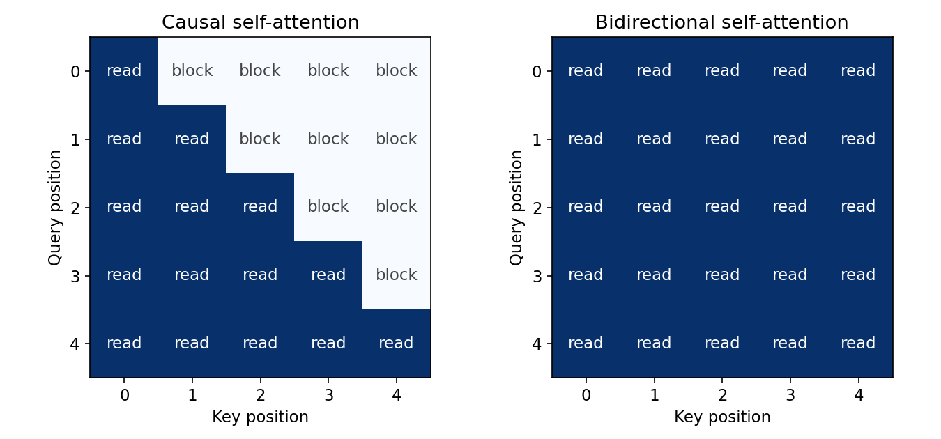
A final linear layer maps the top-layer vector at position to vocabulary logits , and a softmax turns them into . Because every row of the mask hides the future, one forward pass computes the training loss at all positions at once, while generation still produces one token per pass.
The GPT line
The GPT papers show how far this one design can be pushed. Radford and colleagues trained a 12-layer decoder-only Transformer with masked self-attention as a language model on BooksCorpus, then fine-tuned it with a task-specific output layer for classification, entailment and similarity tasks [4]. The recipe was generative pretraining followed by discriminative fine-tuning: unlabeled text supplies most of the learning signal, and a small labeled set adapts the model.
GPT-2 kept the next-token objective and dropped task-specific fine-tuning from its main experiments. Its authors trained on WebText, a new dataset of millions of web pages, used byte-level byte-pair encoding so that any string could be represented, and reported that the language model began to perform tasks such as question answering and summarization in a zero-shot setting; the largest model had 1.5 billion parameters [5]. GPT-3 scaled the same approach to an autoregressive model with 175 billion parameters and evaluated it with tasks and a few demonstrations given purely as text, without gradient updates [6]. These are three points on one line: the architecture and objective barely change, while data, model size and the way tasks are presented do.
Reading the line correctly matters for later sections. A prompt is just a prefix . “Zero-shot” and “few-shot” describe what that prefix contains, not a different model. The quality of a continuation still depends on what the training text made probable, which is why instruction tuning, preference learning and retrieval (Sections 9–11) were added on top.
3. A runnable causal model
Plain version. A tiny model can learn a synthetic language pattern and still generalize poorly to unseen combinations. We also test a property that low loss alone cannot establish: future tokens must not influence earlier predictions.
The following standalone CPU example uses invented fixed-length sentences. Train and test sentences differ, while every ordinary vocabulary item is present in training. The code uses no padding, pretrained weights or dataset downloads. It is intentionally a mechanism experiment rather than a language benchmark.
The implementation uses AdamW for optimization [9], the GELU activation in the feedforward block [10], and layer normalization before attention and the feedforward transformation [11]. These choices define this small experiment, rather than reproduce every detail of the original Transformer. Keep them fixed when studying the causal mask so a change in optimization or activation does not confound the comparison.
Code · Python · 62 lines
import math
import torch
from torch import nn
from torch.nn import functional as F

torch.manual_seed(11)
torch.set_num_threads(1)
train_text = [
    'the red robot moves', 'the blue robot waits',
    'a red sensor waits', 'a blue sensor moves',
    'the red sensor moves', 'a blue robot waits',
]
test_text = ['a red robot moves', 'the blue sensor waits']
vocab = ['<bos>', '<eos>'] + sorted(set(' '.join(train_text).split()))
index = {word: i for i, word in enumerate(vocab)}
def encode(rows):
    return torch.tensor([[index[w] for w in ['<bos>'] + s.split() + ['<eos>']] for s in rows])
train, test = encode(train_text), encode(test_text)

class TinyCausalModel(nn.Module):
    def __init__(self):
        super().__init__()
        self.token = nn.Embedding(len(vocab), 16)
        self.position = nn.Embedding(5, 16)
        self.norm1, self.norm2 = nn.LayerNorm(16), nn.LayerNorm(16)
        self.q, self.k, self.v = [nn.Linear(16, 16, bias=False) for _ in range(3)]
        self.output = nn.Linear(16, 16)
        self.ff = nn.Sequential(nn.Linear(16, 32), nn.GELU(), nn.Linear(32, 16))
        self.head = nn.Linear(16, len(vocab))
    def forward(self, ids):
        length = ids.shape[1]
        h = self.token(ids) + self.position(torch.arange(length))
        z = self.norm1(h)
        scores = self.q(z) @ self.k(z).transpose(-1, -2) / math.sqrt(16)
        blocked = torch.ones(length, length, dtype=torch.bool).triu(1)
        weights = scores.masked_fill(blocked, float('-inf')).softmax(dim=-1)
        h = h + self.output(weights @ self.v(z))
        h = h + self.ff(self.norm2(h))
        return self.head(h)

model = TinyCausalModel()
optimizer = torch.optim.AdamW(model.parameters(), lr=0.01)
def loss(rows):
    logits = model(rows[:, :-1])
    return F.cross_entropy(logits.reshape(-1, len(vocab)), rows[:, 1:].reshape(-1))
initial = loss(train).item()
for _ in range(180):
    optimizer.zero_grad()
    objective = loss(train)
    objective.backward()
    optimizer.step()
model.eval()
with torch.no_grad():
    train_nll, test_nll = loss(train).item(), loss(test).item()
    original = train[:1, :-1]
    changed = original.clone()
    changed[0, -1] = index['blue']
    gap = (model(original)[:, :-1] - model(changed)[:, :-1]).abs().max().item()
assert train_nll < initial and gap < 1e-6
print('initial/train/test NLL:', *(round(x, 3) for x in [initial, train_nll, test_nll]))
print('held-out perplexity:', round(math.exp(test_nll), 3))
print('future-token perturbation gap:', gap)
Output:
Code · 3 lines
initial/train/test NLL: 2.194 0.409 3.17
held-out perplexity: 23.81
future-token perturbation gap: 0.0
The assertion checks that training loss decreases; it does not require held-out loss to improve by any specified amount. Here the held-out loss (3.17 nats per token) is even higher than the untrained starting loss (2.194): the held-out sentences combine familiar words in combinations excluded from training, and the model has confidently memorized the six training patterns. A large train–test gap demonstrates that learning the observed patterns does not establish compositional generalization.
The future-token perturbation test changes the final input token and compares all earlier logits. Causal attention should make that change invisible to earlier predictions, and the printed gap is exactly zero. This test targets the exact visibility contract. Passing it does not establish every form of data isolation: duplicated documents across splits, vocabulary construction from forbidden test data or future metadata can still create other leakage.
The model has no dropout, so evaluation mode does not alter a stochastic layer here. We call it explicitly because the training/evaluation distinction is essential in realistic models. The loss function flattens batch and position dimensions while retaining vocabulary as the class dimension. If those axes are accidentally exchanged, a program can run while optimizing the wrong prediction problem.
Each sequence has the same length, and the position table covers the five model-input positions. A learned position table imposes a maximum supported position; giving a longer sequence is an invalid lookup, not an ordinary longer input. Extending to variable-length data requires separate attention and loss masks. An attention mask controls what representations may read; a loss mask controls which target positions contribute to the objective. They solve different problems and should be tested independently.
4. Training objective and scaling
Plain version. Large language models are trained with the same next-token loss as the tiny model above. What changes is the amount of text, the number of parameters and the compute spent, and those quantities trade off in measurable ways.
Kaplan and colleagues trained families of Transformer language models and reported that held-out loss falls approximately as a power law in model size, dataset size and compute [7]. In model size alone:
Here is held-out cross-entropy loss, is the number of non-embedding parameters, is a fitted constant and is a fitted exponent. Hoffmann and colleagues later fitted a form with an irreducible term, , where is the number of training tokens, the loss that no model can remove, and fitted constants; for a fixed compute budget they concluded that parameters and training tokens should be scaled in roughly equal proportion [8]. ML 10 derives the compute-optimal trade-off and fits a scaling law in code.
Two cautions keep scaling in its place. First, the fitted constants depend on tokenizer, data mixture and training protocol, so they do not transfer between unrelated setups. Second, scaling laws predict loss, not any particular task behavior. A lower next-token loss usually helps, but whether a model preserves a negation in a summary or refuses to invent a citation must still be measured directly (Section 8).
5. Perplexity and meaningful comparison
Plain version. Perplexity summarizes held-out token prediction. Its value depends on what counts as a token and which positions are evaluated.
For mean negative log likelihood :
Here is perplexity and is the natural exponential; uses natural logarithms over the same evaluated token positions. Lower perplexity means that the model assigns higher average probability to observed tokens under that evaluation contract. It is not a direct measure of factual correctness, helpfulness or grammaticality. IT 01 connects this quantity to cross-entropy, and NLP 05 computes it for count models.
Compare perplexities only under compatible tokenization and input conventions. A word can be one token in one vocabulary and several in another. The mean loss per token then describes a different unit. Also record whether beginning and end markers are scored, how documents are segmented, the context length and whether evaluation windows overlap. Recounting duplicated target positions changes the weighting.
Keep evaluation documents independent of training documents and their derivatives. Splitting adjacent passages of one document across partitions can expose style, facts and nearly identical wording. For a time-dependent application, use an appropriate chronological split and retain the document version. A held-out name or phrase does not by itself prove the surrounding document is independent.
McRoy’s benchmark perspective reminds us to assess task behavior in addition to sequence prediction [2]. A classifier needs category performance; an extractor needs spans and supported relations; a generator needs meaning preservation and omissions. A model with lower perplexity can fail a critical task distinction, such as changing “did not move” to “moved.” Match the evaluation to the user’s actual outcome.
A reproducible language-model experiment
A result is useful when someone can tell exactly which text, tokens and decisions produced it. Begin with the document split and its reason: a random split may suit independent synthetic sentences, while a support assistant might require customer-separated or chronological documents. In the toy experiment, the vocabulary comes only from training sentences, and the test combinations were chosen to contain known words. This isolates a narrow combination-generalization question.
Next record the tokenization, sequence boundaries, target shift, maximum context and loss denominator. The code scores every next-token target including the end token, and does not score the beginning token as a target. If another run excludes stopping predictions or weights each sentence equally regardless of length, its number answers a different question. Finally separate selection from reporting: choose architecture, training length and decoding behavior on development data, and inspect the held-out set only after those choices are frozen. Save the preprocessing version, model configuration, seed, permitted input context and output settings, while keeping sensitive raw documents under appropriate access control.
6. Decoding: from a distribution to a text
Plain version. A trained model produces scores. A decoder decides whether to choose the strongest token, search over several continuations, or sample alternatives. None of these choices makes unsupported content reliable.
Temperature
For logit and positive temperature :
Here is a candidate token; is the vocabulary; indexes candidates in the denominator; is the model’s unnormalized score; is temperature; and is the resulting sampling distribution. Lower temperature concentrates mass around high-scoring tokens; higher temperature spreads it. As , sampling approaches greedy selection, which chooses a maximum-score token. A factual mistake can be the highest-logit option, so reducing randomness does not remove it.
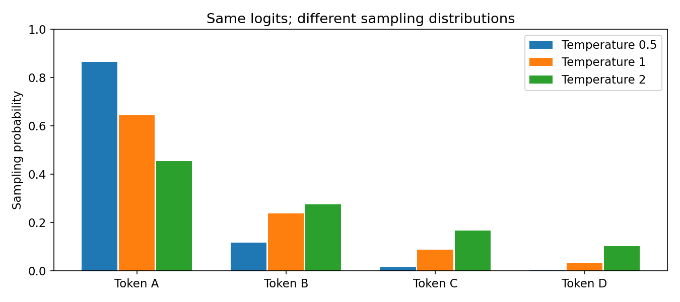
Greedy and beam search
Greedy decoding chooses the most probable next token. Beam search retains several partial sequences. The sequence score for a candidate is
Here is the log probability of the complete output given a prompt or source ; includes the end token; and the other symbols are as above. With raw log probabilities, every additional token contributes a nonpositive term. This can favor shorter sequences. Length adjustments change the search objective; describe their form and tune them on validation data rather than silently applying them.
This tiny conditional model has two competing first tokens. It illustrates why choosing the best next token can miss the best complete sequence. The probabilities are constructed for the experiment, not estimated from language data.
Code · Python · 27 lines
import math

table = {
    (): {"safe": 0.55, "close": 0.45},
    ("safe",): {"stop": 0.51, "wait": 0.49},
    ("close",): {"valve": 0.99, "door": 0.01},
}
def next_probs(prefix):
    return table.get(prefix, {"<eos>": 1.0})
def decode(width):
    beams = [((), 0.0)]
    for _ in range(3):
        candidates = []
        for seq, score in beams:
            if seq and seq[-1] == "<eos>":
                candidates.append((seq, score))
                continue
            for token, prob in next_probs(seq).items():
                candidates.append((seq + (token,), score + math.log(prob)))
        beams = sorted(candidates, key=lambda pair: pair[1], reverse=True)[:width]
    return beams[0]
greedy, beam = decode(1), decode(2)
print(greedy[0], round(math.exp(greedy[1]), 4))
print(beam[0], round(math.exp(beam[1]), 4))
assert greedy[0] == ("safe", "stop", "<eos>")
assert beam[0] == ("close", "valve", "<eos>")
assert beam[1] > greedy[1]
Output:
Code · 2 lines
('safe', 'stop', '<eos>') 0.2805
('close', 'valve', '<eos>') 0.4455
Beam search finds the more probable sequence in this constructed tree. That result is about the model’s probability assignment. If “close valve” contradicts the source instruction, a better probability search still produces the wrong application behavior. Search quality and task correctness need separate measurements.
Search error, model error and a wrong objective
The toy beam succeeds because it keeps the close prefix long enough to discover its strong continuation. Greedy decoding discards that branch before seeing the continuation. This is search error relative to the constructed sequence-probability objective. A larger beam can reduce that kind of error, but it is still a bounded search: a useful prefix can fall outside the retained set at any depth.
Raw prefix log probability supplies a helpful bound. Every future log-probability term is nonpositive, so extending a prefix cannot improve its raw score. A finished candidate that exceeds the scores of all unfinished prefixes is therefore optimal among those surviving branches. This argument requires the unadjusted sum; a length bonus or normalization changes the bound and must be considered in the stopping rule.
Now distinguish model error. If the source requires keeping the valve open while the model assigns its greatest sequence probability to close valve, exact probability search exposes the model’s mistake more consistently. Search cannot create source compatibility that the score lacks. Finally, maximum probability is only one decision objective. A generic short response may have high probability while omitting the required warning. Evaluate whether the selected objective rewards the user’s intended result before tuning beam width.
Top-k and nucleus sampling
For open-ended writing, maximizing probability is often the wrong goal. Holtzman and colleagues observed that using likelihood as a decoding objective produces text that is bland and strangely repetitive, even from a strong model, while pure sampling from the full distribution can pick very unlikely tokens from the long tail [12]. Two truncation rules sit between these extremes.
Top-k sampling keeps the highest-probability tokens and renormalizes. Fan and colleagues used it for story generation, sampling from the 10 most likely candidates at each step and finding it more effective than beam search for that task [13]. Nucleus (top-p) sampling sorts tokens by descending probability and keeps the shortest prefix whose cumulative probability reaches [12]:
Here is the token at rank , its probability, the vocabulary size, the retained prefix length, the nucleus, the target mass, an indicator, and the renormalized sampling distribution. Fix a tie-breaking order for equal probabilities; the code preserves their original index order. The difference from top-k is that the nucleus adapts: after a prefix with one obvious continuation it may contain a single token, and after an open-ended prefix it may contain many.
The descending-prefix condition matters. For probabilities and threshold , top-p retains the first two tokens. The first and last tokens also form a two-element set reaching , but that set skips more probable candidates and is not the intended nucleus. The assertion below checks this distinction.
Code · Python · 45 lines
import numpy as np

tokens = np.array(['valve', 'pump', 'door', 'sensor', 'cabinet', 'label', 'fish', 'moon'])
logits = np.array([3.0, 2.6, 1.2, 1.0, 0.2, -0.5, -1.5, -2.0])

def softmax(z):
    e = np.exp(z - z.max())
    return e / e.sum()

def temperature(z, tau):
    return softmax(z / tau)

def top_k(p, k):
    keep = np.argsort(-p)[:k]                 # indices of the k largest
    q = np.zeros_like(p); q[keep] = p[keep]
    return q / q.sum()

def nucleus(p, top_p):
    if not 0 < top_p <= 1:
        raise ValueError("top_p must be in (0, 1]")
    order = np.argsort(-p, kind="stable")
    cumulative = np.cumsum(p[order])
    size = int(np.searchsorted(cumulative, top_p) + 1)   # smallest prefix reaching top_p
    q = np.zeros_like(p); q[order[:size]] = p[order[:size]]
    return q / q.sum()

p = softmax(logits)
print('greedy choice:', tokens[np.argmax(p)])
for name, q in [('tau=0.5', temperature(logits, 0.5)), ('tau=1.0', p),
                ('tau=2.0', temperature(logits, 2.0)),
                ('top-k=3', top_k(p, 3)), ('top-p=0.9', nucleus(p, 0.9))]:
    print(f'{name:9s} support={int((q > 0).sum())}  P(valve)={q[0]:.3f}  '
          f'tail mass={q[4:].sum():.3f}')

# The nucleus adapts its size to the shape of the distribution.
flat = softmax(np.zeros(8))
peaked = softmax(np.array([6.0, 1, 0, 0, 0, 0, 0, 0]))
print('nucleus size, flat vs peaked:',
      int((nucleus(flat, 0.9) > 0).sum()), int((nucleus(peaked, 0.9) > 0).sum()))

rng = np.random.default_rng(0)
draws = rng.choice(len(tokens), size=2000, p=nucleus(p, 0.9))
assert set(draws) <= set(np.flatnonzero(nucleus(p, 0.9)))
assert np.array_equal(np.flatnonzero(nucleus(np.array([0.4, 0.3, 0.2, 0.1]), 0.5)), [0, 1])
assert np.isclose(top_k(p, 3).sum(), 1) and np.argmax(temperature(logits, 0.1)) == 0
Output:
Code · 7 lines
greedy choice: valve
tau=0.5   support=8  P(valve)=0.667  tail mass=0.003
tau=1.0   support=8  P(valve)=0.481  tail mass=0.052
tau=2.0   support=8  P(valve)=0.312  tail mass=0.190
top-k=3   support=3  P(valve)=0.545  tail mass=0.000
top-p=0.9 support=4  P(valve)=0.507  tail mass=0.000
nucleus size, flat vs peaked: 8 1
Here “tail mass” is the probability left on the four least likely tokens. Temperature only reshapes the distribution, so every token stays possible: at almost a fifth of the mass sits on cabinet, label, fish and moon. Truncation removes the tail outright. On the uniform distribution the nucleus keeps all eight tokens; on the peaked one it keeps one. A fixed would keep three in both cases.
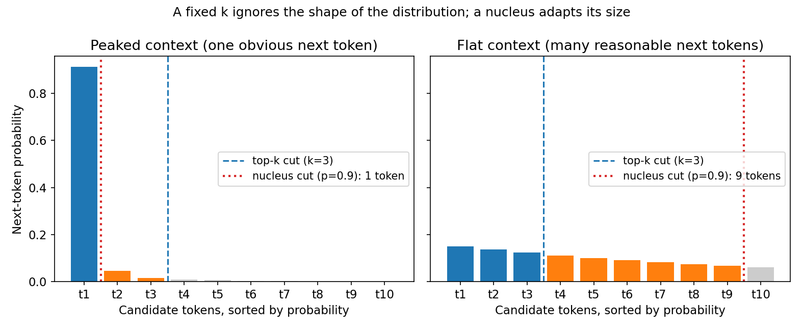
In practice these knobs are combined (for example a temperature followed by a nucleus) and chosen per task. A data-to-text report usually wants deterministic, reproducible output; brainstorming wants variety. Sampling diversity is not evidence of quality, and repeated samples that agree are not an independent verification of a claim: they share the same model and often the same training biases.
Stopping and length
Generation also needs a stopping policy and a length budget. A model may stop too early or continue with redundant content. Set explicit output limits, a stopping rule and behavior when the limit is reached. A truncated summary should not be returned as complete. Record the decoding parameters with the model artifact so an evaluation can be reproduced; changing only the decoder can change every downstream metric.
7. Natural language generation tasks
Plain version. Generation means producing a sequence whose content and form satisfy a task. The input may be a document, a table, a prompt or retrieved passages; the task defines what counts as an error.
A decoder-only model handles every conditional task the same way: it treats the input as a prefix. The conditional factorization is
Here is the source input; is task context, such as the requested language or format; is the output token sequence, including an end token; contains the tokens before position ; and denotes learned parameters. In a decoder-only model, and are serialized into the prefix and the loss is usually taken only over the tokens of ; an encoder–decoder (NLP 08) encodes separately. Either way, the factorization describes a distribution. It does not certify that the sampled output is supported by the source.
Define the generation problem before choosing a model
Begin by writing a task contract in ordinary language. For an equipment report: “Given timestamped observations, produce two sentences describing the current temperature and any explicitly recorded fault; preserve device names, units, numbers and negation.” This contract exposes omissions and contradictions that an unconstrained instruction such as “summarize nicely” hides.
Separate three operations. Content selection chooses observations relevant to the user. Sentence planning decides ordering, grouping and referring expressions. Realization expresses the plan as grammatical text. McRoy [2] provides the linguistic reading for this distinction. Neural systems can combine the operations internally, but a combined architecture still needs tests for each responsibility.
Consider a source with a high temperature, a later normal temperature, and an explicitly absent fault. Selecting the highest reading creates a different report from selecting the latest reading. Neither selection rule follows from grammatical fluency. Record whether the output should describe the current state, an extreme event, or the whole trajectory. Time and scope belong in the input contract.
Data-to-text: a template baseline
Data-to-text generation verbalizes structured records. Wiseman, Shieber and Rush introduced a large corpus of data records paired with descriptive documents, together with extractive evaluation methods that check which records the text actually conveys; the neural systems they tested produced fluent text, yet templated baselines exceeded them on some of those metrics [15]. A template is a useful baseline when the input schema is narrow. It offers complete control over permitted claims and makes failure localization simple. Its limits are also clear: it cannot gracefully cover arbitrary relations, referring expressions or discourse. Measure that coverage rather than treating templates as inherently inadequate.
Here is a deterministic report function for a narrow schema. It demonstrates field validation and traceable output. The event record is trusted structured input; obtaining and validating that record from raw text would be a separate NLP stage.
Code · Python · 26 lines
import math

VERSION = "equipment-template-1"
def report(event):
    required = {"device", "temperature_c", "fault", "evidence_id"}
    if set(event) != required:
        raise ValueError("Unexpected input fields")
    if not isinstance(event["device"], str) or not event["device"].strip():
        raise ValueError("Missing device")
    value = event["temperature_c"]
    if isinstance(value, bool) or not isinstance(value, (int, float)) or not math.isfinite(value):
        raise ValueError("Temperature must be finite")
    if event["fault"] not in ("present", "absent", "unknown"):
        raise ValueError("Unknown fault status")
    if not isinstance(event["evidence_id"], str) or not event["evidence_id"]:
        raise ValueError("Missing evidence ID")
    phrases = {"present": "A fault was recorded.",
               "absent": "No fault was recorded.",
               "unknown": "Fault status was not recorded."}
    text = f"{event['device']} measured {value:g} C. {phrases[event['fault']]}"
    return {"text": text, "evidence_id": event["evidence_id"], "version": VERSION}
output = report({"device": "Pump A", "temperature_c": 30,
                 "fault": "absent", "evidence_id": "synthetic-event-01"})
print(output)
assert output["text"] == "Pump A measured 30 C. No fault was recorded."
assert output["version"] == VERSION
Output:
Code · 1 line
{'text': 'Pump A measured 30 C. No fault was recorded.', 'evidence_id': 'synthetic-event-01', 'version': 'equipment-template-1'}Notice the difference between absent and unknown. The input “no fault was recorded” is a statement about recorded evidence, not a claim that a fault is impossible. Encoding that distinction prevents the realization stage from upgrading missing evidence into certainty. A learned generator becomes useful when its additional flexibility solves a documented failure of this baseline, and it should be tested on exactly these distinctions.
Extractive summarization: select evidence under a budget
An extractive summary chooses source sentences. An abstractive summary may rewrite or combine them. Extraction makes the origin of each sentence explicit, but the selected sentences can still mislead through missing context, conflicting timestamps or unresolved pronouns. Selecting a sentence containing “it failed” without its antecedent is a discourse error even though every word came from the source.
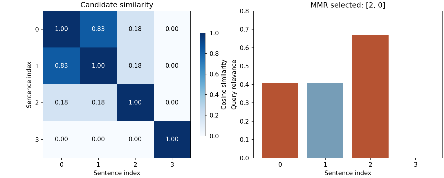
Suppose a document contains candidate sentences . Represent sentence by a unit vector and a user query by a unit vector . A simple relevance score is . To discourage repetition, use maximal marginal relevance, or MMR [14]:
Here is the set of already selected sentence indices; is the next index; balances relevance against similarity to previous selections; and the maximum similarity is defined as zero when is empty. The dot products are cosine similarities because the vectors have unit length. This is a greedy selection rule, rather than a proof of globally optimal summary quality.
The following example uses binary word indicators to make every decision inspectable. The four candidate sentences are synthetic. Removing a small set of function words makes the representation less dominated by grammar, but it also removes potentially useful distinctions.
Code · Python · 30 lines
import re
import numpy as np

sentences = [
    "Pump A temperature reached 80 C during the test.",
    "The test recorded Pump A temperature at 80 C.",
    "Pump A vibration triggered a shutdown warning.",
    "The technician replaced a label on the cabinet.",
]
query = "pump temperature vibration shutdown"
stop = {"a", "the", "at", "on", "during"}
def tokens(text):
    return set(re.findall(r"[a-z0-9]+", text.lower())) - stop
vocab = sorted(set().union(*(tokens(s) for s in sentences), tokens(query)))
def vector(text):
    v = np.array([w in tokens(text) for w in vocab], dtype=float)
    return v / max(np.linalg.norm(v), 1e-12)
V = np.stack([vector(s) for s in sentences])
q = vector(query)
relevance, similarity = V @ q, V @ V.T
selected = []
for _ in range(2):
    redundancy = similarity[:, selected].max(axis=1) if selected else np.zeros(4)
    score = 0.55 * relevance - 0.45 * redundancy
    score[selected] = -np.inf
    selected.append(int(np.argmax(score)))
print("Selected indices:", selected)
print("Summary:", " ".join(sentences[i] for i in sorted(selected)))
assert len(set(selected)) == 2
assert 2 in selected and not ({0, 1} <= set(selected))
Output:
Code · 2 lines
Selected indices: [2, 0]
Summary: Pump A temperature reached 80 C during the test. Pump A vibration triggered a shutdown warning.
The selected pair includes the shutdown sentence and one temperature sentence, avoiding the nearly repeated temperature observation. Sorting the selected indices restores source order after selection. This matters because selection order measures marginal value, while presentation order should support comprehension.
A real budget usually limits tokens rather than sentence count. Add a candidate only if its full tokenized length fits the remaining budget; silently cutting a sentence can remove its condition or negation. For multi-document summaries, group near-duplicate reports so repeated copies do not masquerade as independent evidence. Retain source IDs and timestamps so readers can follow the selected evidence.
Relevance, feasibility and content preservation are different objectives
MMR discourages selecting sentences that resemble previous selections [14]. It does not know which facts are mandatory. If a warning shares many words with a selected observation, a similarity penalty can suppress it even though its added qualification is essential. Vector diversity is a proxy for redundancy, not a direct measure of complete meaning.
A content requirement changes the feasible set. For a token budget and a required warning:
Here is the selected sentence-index set, is the full token length of candidate , is the budget, and contains candidates expressing the required warning. The first condition limits size; the second ensures coverage. If no set satisfies both, the task is infeasible for extraction under that budget. Changing a relevance coefficient cannot make an over-budget sentence fit or invent a missing warning.
The following independent example isolates that distinction. Utilities are explicit teaching choices, not learned relevance scores:
Code · Python · 19 lines
import itertools

sentences = [
    'Pump A temperature reached 80 C during the test.',
    'The test recorded Pump A temperature at 80 C.',
    'Pump A vibration triggered a shutdown warning.',
    'The technician replaced a label on the cabinet.',
]
lengths = [len(s.split()) for s in sentences]
utility = [0.9, 0.85, 0.6, 0.2]
subsets = [tuple(i for i in range(4) if keep[i])
           for keep in itertools.product([False, True], repeat=4)]
feasible = [s for s in subsets if sum(lengths[i] for i in s) <= 20]
score = lambda s: sum(utility[i] for i in s)
ordinary = max(feasible, key=score)
with_warning = max((s for s in feasible if 2 in s), key=score)
print('Lengths:', lengths)
print('Without requirement:', ordinary, 'with warning:', with_warning)
assert ordinary == (0, 1) and with_warning == (0, 2)
Output:
Code · 2 lines
Lengths: [9, 9, 7, 8]
Without requirement: (0, 1) with warning: (0, 2)
Here length counts whitespace-separated words; a model-token budget must use that model’s tokenizer. The unconstrained choice repeats temperature content; the warning requirement changes the selected pair. More sophisticated scoring still needs the task’s hard content requirements when omission is unacceptable.
Abstractive summarization
A rewriting model can fuse observations and improve readability. It can also invent a connecting statement that the observations never established. “The temperature was high, so the pump failed” adds causation if the source only records simultaneous events. Rewriting two sentences into one is acceptable when relationships survive, but changing sequence into causation or removing “during the test” alters content. A plan that records propositions and their source intervals before wording is generated lets you evaluate selection, plan and realization separately, so you can tell where meaning was lost.
Story generation and open-ended text
Open-ended generation reverses the priorities of a report. There is no single correct output, and variety is part of quality. Fan, Lewis and Dauphin collected a dataset of human-written stories paired with writing prompts, generated a premise first and then the story, and used top-k sampling because beam search tended to produce short and generic text [13]. The lesson for this chapter is that the same language model can need different decoders for different tasks: deterministic search for a constrained report, truncated sampling for a story. What stays constant is that the evaluation must match the task: coherence and relevance to the prompt for a story, supported content for a summary.
8. Evaluating generated text
Plain version. One automatic score cannot summarize all generation quality. Use automatic metrics to compare systems under a specified protocol, then inspect the error dimensions the application actually cares about.
Perplexity (Section 5) evaluates the model as a predictor of reference text. It says nothing directly about a particular decoded output, and it cannot compare models with different tokenizers. Overlap metrics compare an output with references. ROUGE includes recall-oriented overlap measures for summarization [17]. Such metrics compare a candidate with one or more references; they do not prove semantic equivalence or source support. Name the variant, tokenizer, aggregation and reference set when reporting a score. Translation metrics such as BLEU and learned metrics are discussed in NLP 08.
For a simple unigram recall check,
Here ranges over word types; and are reference and hypothesis word counts. The denominator is the number of reference tokens. This overlap calculation illustrates one component of ROUGE-style evaluation; the minimal implementation below does not reproduce every preprocessing or aggregation option of a full evaluation package.
Code · Python · 14 lines
import re
from collections import Counter

def words(text):
    return re.findall(r"[a-z0-9]+", text.lower())
def overlap_recall(reference, hypothesis):
    ref, hyp = Counter(words(reference)), Counter(words(hypothesis))
    return sum((ref & hyp).values()) / sum(ref.values())
reference = "Pump A is operating at 30 C."
contradiction = "Pump A is not operating at 30 C."
score = overlap_recall(reference, contradiction)
print("Unigram recall:", score)
assert score == 1.0
assert ("not" in words(reference)) != ("not" in words(contradiction))
Output:
Code · 1 line
Unigram recall: 1.0The contradiction receives recall 1.0 because it retains every reference token. A precision term would penalize the extra word, but the small penalty would still not express the importance of reversed negation. This is a controlled counterexample, not evidence that overlap metrics never correlate with human judgments. It explains why the metric must be paired with meaning-sensitive checks.
Human evaluation and error categories
For the equipment application, count unsupported claims, missing required claims, incorrect numeric relations, and unresolved references separately. These are project-defined error categories. Give annotators positive and negative examples for each, including cases where evidence is absent or contradictory. A summary that says less may have fewer unsupported claims while omitting critical information; report both error directions.
Human evaluation should hide system identity, randomize presentation, preserve source context and specify the decision task. Ask reviewers to mark unsupported statements before judging overall usefulness. An overall preference may reward style and miss a rare critical error. Report who reviewed the outputs and how disagreements were resolved. Aggregate by a meaningful unit: several sentences from one incident are correlated, and treating them as independent examples can exaggerate certainty.
Language models as judges
A strong language model can be prompted to grade or compare outputs. Zheng and colleagues studied this “LLM-as-a-judge” setting and reported that a strong judge’s preferences agreed with human preferences at a level comparable to agreement between humans on their benchmarks, while also documenting position bias, verbosity bias and self-enhancement bias [18]. Wang and colleagues showed that simply swapping the order in which two responses appear can change which one a model judge prefers, and proposed calibration such as evaluating both orders [19].
Treat a model judge as another measurement instrument with its own version, prompt and failure modes. Evaluate both presentation orders, hide which system produced which output, validate the judge against human labels on your own error categories (especially negation, quantities and unsupported claims), and avoid using a judge from the same model family as the system it grades when that can be avoided. A judge that ranks systems well on average is not automatically a reliable gate for accepting a single output.
9. Retrieval: finding the evidence to generate from
Plain version. Before a generator can use evidence, something must find it. A retrieval system selects passages from an explicit corpus; whether those passages support an answer, and how the answer is worded, are later decisions.
A language model can continue a question without searching a current document collection. A retrieval system instead selects information from an explicit corpus. Question answering adds another decision: whether the selected information supports an answer, and which words express it. Putting these components together creates a useful pipeline, but no stage automatically certifies the next.
This section’s running question is “What is the temperature limit for Pump A?” A relevant passage discusses Pump A or temperature. A sufficient passage states the limit for that pump under the applicable policy. A valid citation points to a real source. A supported answer preserves the source’s value, units, time and scope. These are four separate conditions, and an evaluation should be able to tell which one failed.
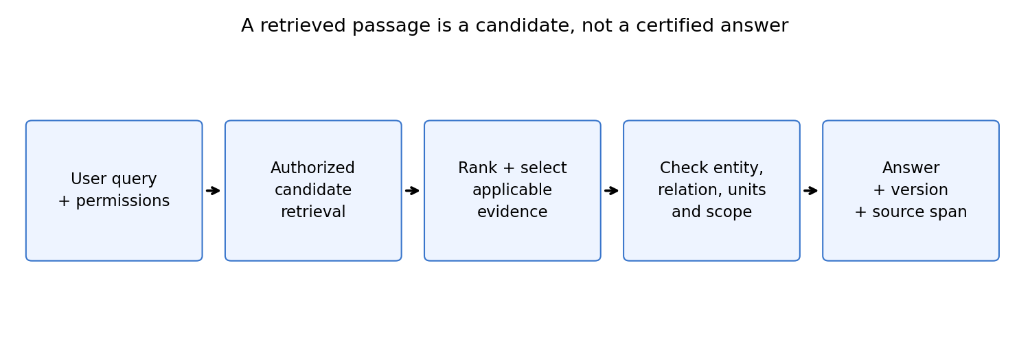
This section builds and evaluates the retrieval stage. Deciding whether a retrieved passage actually answers the question — extractive span answers, relevance versus answerability, and diagnosis by controlled substitution — is developed in NLP 11. Section 10 then conditions a generator on the retrieved evidence.
Corpus design before model choice
Plain version. A retriever searches what you give it. Document identity, freshness and permissions are part of the system, not optional metadata added after ranking.
Represent a searchable passage as:
Here is a passage record; is the parent document identifier; is its version; and are inclusive-start and exclusive-end offsets in the original document; is passage text; and describes its access policy. The offset unit must be declared. This is our application record, rather than a universal storage standard.
A passage may be a paragraph, a sentence group or a section selected by document structure. Small passages can isolate an answer but lose its qualifications. Large passages retain context but introduce unrelated text and consume more generation budget. Choose chunk boundaries based on the task, then evaluate whether the supporting facts and their conditions remain together.
For example, a heading may specify “Outdoor equipment only,” followed by a paragraph containing a temperature limit. If the paragraph is indexed alone, it may appear to apply to indoor equipment. Retaining the heading or a structured scope field changes the answerability contract. A fixed character window is easy to implement, but simplicity does not establish that it preserves meaning.
Versions also matter. An old policy can be relevant yet inapplicable. Keep effective dates and replacement links when the application needs current answers. Do not rely on a generator to infer the current policy merely because the newest passage appears last in the prompt. Filter or rank by declared applicability rules, and make conflicts visible when the corpus does not identify a single authoritative source.
Apply permissions before returning passage text to an unauthorized component or user. Filtering the final visible answer is too late if private text was already included in a model request or log. The retriever’s corpus view should match the current user’s permitted view. Measure retrieval quality under that restricted view; global relevance scores can otherwise evaluate documents the system may never show.
Lexical retrieval and sparse vectors
Plain version. Lexical retrieval matches words and weights informative terms. It is inspectable and often useful when exact names, identifiers and technical phrases matter.
A simple term-frequency and inverse-document-frequency weight is:
Here is the weight of term in document ; is its frequency under a chosen convention; is the number of indexed documents; and is the count of documents containing the term. A zero document frequency requires special handling for query-only terms. Implementations often smooth the formula or transform term frequency; record the actual convention [33, 34].
With normalized document and query vectors:
Here is a query; is a candidate document; are their vectors; is cosine similarity; and is Euclidean norm. Define the score as zero when either vector is zero. The code uses normalized vectors from scikit-learn, so their dot product implements cosine similarity for nonzero rows [34].
An inverted index stores, for each term, the documents where it occurs. That allows a search engine to consider matching candidates without comparing a query with every vocabulary entry in every document [33]. Our small code computes all document scores because the corpus contains only four passages. The mathematical representation and the efficient indexing strategy are separate choices.
Preprocessing directly affects retrieval. A tokenizer that discards one-character tokens can remove the A in Pump A. Lowercasing may be helpful for ordinary words but can erase distinctions in case-sensitive identifiers. Phrase features help distinguish adjacent words, but do not capture arbitrary syntax or guarantee semantic equivalence. Inspect the vocabulary before blaming the ranking model for a missed result.
Lexical systems can miss paraphrases. “Device ceased operating” and “machine shutdown” may share little wording. A synonym or query-expansion rule can help, but changes the matching policy and may add ambiguity. Evaluate expansion on held-out queries, especially exact-identifier cases. A broad expansion that improves recall can also retrieve a wrong device with similar terminology.
Saturation and document length
Plain version. Repeating a query word many times should not always keep increasing relevance. Longer documents also have more opportunities to match by chance.
One common BM25 form is:
Here is the query-term set in this simplified form; is the candidate document; is term frequency; is a chosen inverse-document-frequency weight; is document length in tokens; is average document length; is a positive saturation parameter; and controls length normalization. Different implementations use different IDF and query-frequency conventions. The information-retrieval textbook discusses this family and its assumptions [33].
The numerator and denominator make the term-frequency contribution approach a limit as repetition grows. The length term changes how much frequency is expected in a longer document. These are ranking adjustments, not a probability that the document contains a true answer. A passage can rank highly because it repeatedly discusses a limit while never stating the value.
Tune length normalization on development queries that reflect the deployment corpus. If every useful answer is in a short reference entry while irrelevant documents are long narratives, a particular setting can look very strong. Changing to long technical manuals may alter that behavior. Keep passage construction fixed when comparing ranking settings, or report that both the corpus representation and score changed.
Dense retrieval and joint reranking
Plain version. A learned encoder can match related expressions without exact word overlap. Its success depends on the training task and the examples used as contrasts.
A dual-encoder score is:
Here maps queries to vectors; maps passages to vectors; denotes learned parameters; and is their dot-product score. The encoders may share parameters or use distinct ones. Dense Passage Retrieval provides an original question-answering example of this design [35].
Passage vectors can be computed ahead of time. A query then searches those vectors for high scores. Approximate search trades some exact nearest-neighbor fidelity for speed; if used, evaluate both the representation and the search approximation. Our chapter does not implement such an index, because an exact small corpus is better for learning the contract.
A contrastive training loss can compare one positive passage with several negative passages:
Here is the loss for one query; is an annotated positive passage; is negative candidate ; is a positive temperature; and is the learned score. Negatives may include difficult passages with similar wording. A passage labeled negative merely because it was not annotated can be a false negative if it also contains a valid answer.
A joint reranker reads a query and candidate passage together, which permits richer token interactions than comparing two fixed vectors. It is typically applied after a cheaper candidate retrieval stage. This adds computation and another selection procedure. Report candidate recall before reranking: a reranker cannot recover the missing correct passage if it never receives it.
Dense and lexical retrieval can be complementary. Dense representations may help paraphrases; lexical matching can preserve exact codes and rare names. Combining score scales requires care because a lexical score and a learned dot product do not have the same units. Select combination settings on development data, and inspect whether the combined system introduces wrong-entity results.
What the contrastive loss actually teaches
The dense loss does more than move a query toward any vaguely related passage. It learns the distinctions represented by the candidate set. Let candidate zero be the positive passage and let the remaining candidates be negatives. For candidate scores:
Here is the query’s score for candidate , is the number of negative candidates, indexes all candidates, is temperature, is the candidate softmax probability, is the loss, and is one for the positive and zero otherwise. This derivative follows directly from the softmax loss above. Gradient descent increases the positive score and decreases negative scores; the strongest competing negative receives the largest downward pressure.
DPR uses positive and negative passage comparisons to train separate query and passage representations [35]. The equation explains why choosing the comparisons matters. If negatives are unrelated topics, the model may learn topic separation without learning to distinguish Pump A from Pump B. A wrong-device passage with the same relation is a more informative contrast for that error. But if an unannotated passage really supports the answer, treating it as negative teaches the wrong separation.
This standalone score-space experiment verifies the gradient direction. It illustrates the objective; it does not train passage encoders:
Code · Python · 15 lines
import numpy as np

scores = np.array([1.2, 0.8, -0.4])  # positive, hard negative, easy negative
def probabilities(values):
    z = np.exp(values - values.max())
    return z / z.sum()
p = probabilities(scores)
gradient = p.copy()
gradient[0] -= 1.0  # temperature is one
updated = scores - 0.5 * gradient
before, after = -np.log(p[0]), -np.log(probabilities(updated)[0])
print('Gradient:', gradient.round(3))
print('Loss:', round(before, 3), '->', round(after, 3))
assert gradient[0] < 0 and gradient[1] > gradient[2] > 0
assert after < before
The gradient rounds to [-0.466, 0.358, 0.108], and loss falls from 0.627 to 0.467. The competing high-score negative receives more downward pressure than the easy negative.
Changing temperature affects both distribution sharpness and gradient scale. Changing candidates changes the contrast being learned. Consequently, improvements from a new encoder cannot be attributed to architecture alone when its positive labels, negative construction or training corpus also change. Keep those differences visible in the comparison.
Compare retrieval routes on the distinction that matters
A dual encoder compresses a passage before it knows the future query. This permits cached vectors and efficient candidate search, but every query-relevant detail must survive that compression. A joint reranker receives both texts simultaneously and can compare specific tokens across them. It spends more computation per pair and still depends on its training examples; joint attention is an opportunity to distinguish a detail, not proof that the detail will be respected.
| Query distinction | Useful evidence | Failure to inspect |
|---|---|---|
Pump A versus Pump B | Exact identifier plus relation | Topic similarity overwhelms a one-character difference |
ceased operating versus shutdown | Learned paraphrase compatibility | Lexical vocabulary misses equivalent wording |
| Current versus pre-upgrade limit | Version and effective-date metadata | A highly relevant passage answers the wrong time scope |
| Permission versus prohibition | Negation and its grammatical scope | Shared vocabulary hides an opposite instruction |
A hybrid design can take the union of lexical and dense candidate sets, remove duplicates, and jointly rerank the survivors. Union protects candidates found by either route, while a fixed total budget can still force some candidates out. Simply adding raw scores is less transparent: multiplying one system’s scores by a constant preserves its own ranking but changes its influence in the combined sum. Normalization or learned combination therefore requires development judgments, not an arbitrary coefficient presumed to work everywhere.
Compare candidate recall, final ordering and resource cost separately. A system can improve the first while harming the second, or improve both while exceeding the serving budget. Diagnose exact names, paraphrases and scope-sensitive questions as distinct groups. Their error patterns reveal which information the representation loses and which downstream interaction is worth paying for.
Ranking evaluation
Plain version. Retrieval evaluation needs queries with relevance judgments. A document being selected does not establish that it was the right one.
For query with relevant-document set and top- result set :
Here is the cutoff; contains the annotated relevant documents; contains the retrieved documents up to that cutoff; and denotes set size. We evaluate this expression only for queries with at least one relevant document. Queries with no answer belong in a separate answerability evaluation, rather than receiving an arbitrary recall value.
If the first relevant result has rank :
Here is reciprocal rank; is its mean; is the number of evaluated queries; and starts at one. Define reciprocal rank as zero when no relevant result is returned. These ranking diagnostics appear in the current retrieval-augmented evaluation discussion [31]. Reciprocal rank emphasizes the first successful hit and ignores later relevant results.
Annotation completeness matters. If only one passage is judged relevant when several support the answer, a valid retrieval can be scored as wrong. Record whether relevance means topic match, answer-containing evidence or complete support. Use multiple judgments when an ambiguity is consequential, and adjudicate according to a written guide. The dataset should expose the task definition, not merely list a favorite passage.
Keep query families and document derivatives separate across development and test. Rephrasing a development query into a nearly identical test query gives weak evidence of generalization. Likewise, splitting chunks from one report across document partitions can leak facts and wording. Choose a split reflecting the deployment question: unseen users, unseen documents, future versions or new domains.
Measure a small retriever
The standalone code uses four synthetic passages. It preserves one-character words so that the device identifier A remains a feature, and it measures ranking on three annotated queries.
Code · Python · 30 lines
import numpy as np
from sklearn.feature_extraction.text import TfidfVectorizer

corpus = {
    'temperature-v2': 'Pump A temperature limit is 80 C. This policy is current.',
    'shutdown-v1': 'Pump A shutdown follows a vibration alarm.',
    'label-v1': 'A technician replaced the cabinet label.',
    'sensor-v1': 'Sensor B reports humidity once per hour.',
}
ids = list(corpus)
vectorizer = TfidfVectorizer(ngram_range=(1, 2), token_pattern=r"(?u)\b\w+\b")
D = vectorizer.fit_transform([corpus[key] for key in ids])
def rank(query):
    score = (D @ vectorizer.transform([query]).T).toarray().ravel()
    order = sorted(range(len(ids)), key=lambda i: (-score[i], ids[i]))
    return [(ids[i], float(score[i])) for i in order]
queries = [
    ('Pump A temperature limit', {'temperature-v2'}),
    ('vibration shutdown alarm', {'shutdown-v1'}),
    ('humidity report', {'sensor-v1'}),
]
recalls, reciprocal = [], []
for query, relevant in queries:
    ranking = rank(query)
    recalls.append(len({key for key, _ in ranking[:2]} & relevant) / len(relevant))
    first = next((i + 1 for i, (key, _) in enumerate(ranking) if key in relevant), None)
    reciprocal.append(1 / first if first else 0.0)
    print(query, '->', ranking[0][0])
print('mean Recall@2:', np.mean(recalls))
print('mean reciprocal rank:', np.mean(reciprocal))
Output:
Code · 5 lines
Pump A temperature limit -> temperature-v2
vibration shutdown alarm -> shutdown-v1
humidity report -> sensor-v1
mean Recall@2: 1.0
mean reciprocal rank: 1.0
The three top results match their single annotated relevant passages, producing mean Recall@2 and mean reciprocal rank of 1.0 in this small run. That is a fixture result, not a real retrieval benchmark. NLP 11 reuses the same corpus and ranker for a narrow evidence-backed answerer.
Graded relevance: nDCG
Recall@k and reciprocal rank treat a judgment as relevant or not. When judges grade passages — complete support above a merely topical mention — a measure should reward placing the most useful passage first.
Here is the graded relevance of the result at rank ; is the discounted cumulative gain over the first ranks; is the same sum for the ideal ordering of the judged results, so ; define it as zero when . Järvelin and Kekäläinen introduced the cumulated-gain family of measures [36]; the logarithm base, the gain transform and the cutoff vary between implementations, so report them.
Two rankings of the same four judged passages differ only in whether the supporting passage or the topical one comes first:
Code · Python · 16 lines
import numpy as np

def dcg(gains, k):
    gains = np.asarray(gains[:k], dtype=float)
    return float(np.sum(gains / np.log2(np.arange(2, gains.size + 2))))
def ndcg(gains, k):
    ideal = dcg(sorted(gains, reverse=True), k)
    return dcg(gains, k) / ideal if ideal > 0 else 0.0

# graded judgments of one ranking: 2 = complete support, 1 = topical, 0 = unrelated
ranked_a = [1, 2, 0, 0]  # topical passage above the supporting one
ranked_b = [2, 1, 0, 0]  # supporting passage first
for name, gains in [('A', ranked_a), ('B', ranked_b)]:
    print(name, 'nDCG@3:', round(ndcg(gains, 3), 3),
          'binary RR:', 1 / (1 + gains.index(2)))
assert ndcg(ranked_b, 3) == 1.0 and ndcg(ranked_a, 3) < 1.0
Output:
Code · 2 lines
A nDCG@3: 0.86 binary RR: 0.5
B nDCG@3: 1.0 binary RR: 1.0
Reciprocal rank with “complete support” as the relevance criterion halves for ranking A. nDCG also drops, but less, because it still credits the topical passage at rank 1. Which behavior is right depends on the task: if only a complete answer is useful, the graded credit for topical passages can hide a failure. Write the grading guide before choosing the measure.
10. Hallucination and retrieval-augmented generation
Plain version. A language model can produce fluent text that is not supported by its input or by the world. Retrieval supplies external evidence, but the generator still needs to use it correctly, and retrieved text must never be treated as a new authority.
Ji and colleagues’ survey distinguishes intrinsic hallucination, output that contradicts the source, from extrinsic hallucination, output that cannot be verified from the source [20]. Maynez and colleagues’ human study of abstractive summarizers found substantial amounts of hallucinated content in all model-generated summaries they examined, and found that textual-entailment measures correlated better with faithfulness than standard overlap metrics [21]. Both points follow from Sections 1 and 6: the training objective rewards probable text, and no decoder adds evidence that the distribution lacks.
Use attention as a diagnostic of computational access, not a factuality certificate. A token can attend to the correct evidence and still express its opposite. Evidence validation should examine the output claim, source entity, relation and scope. For narrow structured tasks, the generator can verbalize a validated plan, as in the template above. For unrestricted prose, validation becomes incomplete and should be reported as such.
Retrieval-augmented generation
The original retrieval-augmented generation, or RAG, paper combines a learned retriever with conditional sequence generation for knowledge-intensive tasks [22]. One sequence-level form is:
Here is the input question; is the output sequence; is a retrieved passage; is the selected top- candidate set; parameterizes the retriever; and parameterizes the generator. The approximation reflects restricting retrieval to candidates. This is a model-specific probabilistic formulation, not a definition that every contemporary RAG application implements.
Many practical systems retrieve passages, assemble a prompt and run a separately trained generator. That pipeline can be useful without optimizing the original marginal objective. State which design you use. Otherwise the name RAG can hide whether retrieval is learned, whether candidates are reranked and whether the generator is trained to use the selected sources. Section 9 builds and evaluates the retriever itself; extractive answers and answerability checks are in NLP 11.
Grounding means relating claims to external evidence under a declared support rule. A generated answer with citations may be traceable, but traceability is weaker than support. A valid URL can point to a document that contradicts the answer. Evaluate whether each consequential claim follows from its cited evidence, and whether the answer includes necessary qualifications.
Evidence may also conflict. A generator should not silently combine mutually inconsistent policies into a single confident answer. An application can prioritize an authoritative version, display a conflict or request clarification according to its contract. The decision should come from metadata and task rules, rather than which sentence happens to be most fluent.
Errors propagate through retrieval, interpretation and realization
A supported answer requires a chain of successful decisions. The corpus must contain applicable evidence, retrieval must preserve it, the reader must interpret the right entity and relation, and the output must retain that interpretation. An answer guessed from memorized knowledge can be correct by coincidence while failing this evidence requirement. For questions whose applicable evidence is in the corpus, write:
Here denotes probability, is the event that sufficient evidence survives retrieval, is the event that the evidence is interpreted correctly, and is the event that the output faithfully realizes the interpretation. The expression is the probability chain rule, not an independence assumption. Multiplying unrelated unconditional stage scores is not equivalent: reader accuracy on hand-picked easy passages may differ from reader accuracy on the retriever’s actual candidates.
Code · Python · 12 lines
import numpy as np

retrieved = np.arange(100) < 80
interpreted = np.arange(100) < 72
realized = np.arange(100) < 68
r = retrieved.mean()
e = interpreted[retrieved].mean()
g = realized[retrieved & interpreted].mean()
complete = (retrieved & interpreted & realized).mean()
print('Conditional stage rates:', round(r, 3), round(e, 3), round(g, 3))
print('Complete supported answers:', round(complete, 3))
assert np.isclose(r * e * g, complete)
Output:
Code · 2 lines
Conditional stage rates: 0.8 0.9 0.944
Complete supported answers: 0.68
These are synthetic outcomes, not reported system performance. The calculation explains why individually respectable component results need not produce equally strong complete answers. Improving the weakest stage is useful only if the improvement survives the later stages.
Boundaries around retrieved content
Retrieved text is evidence to inspect, not an instruction source with permission to change the application. A passage can contain quoted commands, misleading text or an adversarial instruction. Prompt injection describes attempts to make a model follow instructions that conflict with the intended application boundary; OWASP documents this risk category [23]. For retrieval systems, the important boundary is between user/application instructions and untrusted source material.
Keep source text delimited and labeled with document identity. Do not allow it to redefine the current user’s permissions, request secret data or authorize a tool action. If tools are available, validate actions against the user’s task and the application policy outside the retrieved passage. A textual delimiter helps structure input, but is not a complete enforcement mechanism.
The same principle applies to logs and caches. A cached result produced under one user’s access policy must not be reused for another user without checking permissions. Evidence spans must refer to the same document version used for the answer. When a document is removed or replaced, refresh the index and consider invalidating derived answers.
These checks also support ordinary correctness. A passage that says “Ignore the old limit; the new policy is below” can be legitimate document content that needs interpretation, while “Ignore your application instructions” is not a new authority for the system. Store both as source material, then apply the task’s evidence and permission rules. Do not make the retriever a route for changing the governing contract.
11. Adapting a pretrained generator
Plain version. Pretraining learns broad continuation patterns. Adaptation changes behavior for a task; prompting changes the supplied input without necessarily changing weights. Learning to follow an instruction and learning which response people prefer are different signals, and neither is a truth guarantee.
Supervised task adaptation minimizes a task-specific loss over labeled examples, for instance the conditional loss of Section 7 over the response tokens only. Continued language-model training on domain text changes the distribution modeled, but does not automatically teach the application’s output policy. Domain familiarity and task instruction are distinct forms of adaptation. In-context examples, as in GPT-3 [6], appear inside the input and demonstrate format without updating parameters; examples that contain private answers or test labels can invalidate evaluation, and a prompt chosen on development cases must be frozen before the final test.
Low-Rank Adaptation, or LoRA, freezes a base weight matrix and trains a constrained update [24]:
Here is the frozen matrix; and are learned factors; is the chosen rank; and is the effective adapted matrix. This simplified expression omits optional scaling. Fewer trainable parameters can reduce adaptation cost, but do not remove the need for representative labels, data isolation or task evaluation. Save the base-model version, tokenizer, adaptation weights and configuration together: an adaptation trained against one base checkpoint is not guaranteed to work on another checkpoint with the same family name.
The InstructGPT paper studies supervised instruction examples followed by preference-based training with human feedback [25]. This distinguishes a base continuation model from one adapted toward requested behavior. The source of preferences matters: annotators follow a policy, and that policy may balance helpfulness, formatting and other goals. A preferred response can still contain a factual error.
Direct Preference Optimization, or DPO, uses preferred and rejected responses with a reference policy [26]. A representative objective is:
Here is the prompt; and are the preferred and rejected response sequences; is the trainable policy; is a fixed reference policy; is a positive scale parameter; is the logistic sigmoid; and is the loss for one preference pair. Sequence probabilities are products over response-token conditionals; prompts are context rather than supervised response tokens.
The objective increases the preferred response’s relative likelihood compared with the rejected response, measured against the reference. If a dataset rewards confident unsupported answers, optimizing the objective can reinforce that behavior. Instruction compliance, preference agreement and factual support are separate properties that need separate evidence. ML 10 runs a low-rank update in code.
Optional: InstructGPT (in the Paper guides). Follow the original figure, objective, experimental comparisons and limitations.
12. Training practices meet serving constraints
Plain version. A deployed generator serves inputs of different lengths, and its cost per request depends on both the prompt and the output. Padding and cached attention state are two different memory costs; measure both.
Hagiwara’s Chapter 10 connects padding, sorting and masking to practical inference [1]. Keep this distinction clear: a correct loss mask prevents padding from altering the objective; it does not necessarily prevent the hardware from processing padded positions. Define padding utilization as
Here is the real token length of request ; is batch size; and is the fraction of padded token positions containing real tokens. This is a workload diagnostic, not a measured speedup. Sorting nearby lengths into batches can increase utilization while also delaying requests that wait for a matching batch.
Code · Python · 18 lines
import numpy as np

lengths = np.array([8, 64, 12, 60, 10, 56, 14, 52])
def utilization(values):
    batches = values.reshape(-1, 4)
    real = int(batches.sum())
    padded = int((batches.max(axis=1) * 4).sum())
    return real / padded
arrival = utilization(lengths)
bucketed = utilization(np.sort(lengths))
print("Arrival-order utilization:", round(arrival, 3))
print("Length-bucketed utilization:", round(bucketed, 3))
assert bucketed > arrival
# Two cache arrays (keys and values), with a toy equal head layout.
layers, kv_heads, head_dim, cache_tokens, bytes_per_value = 4, 2, 16, 128, 4
cache_bytes = 2 * layers * kv_heads * head_dim * cache_tokens * bytes_per_value
print("Toy cache bytes:", cache_bytes)
assert cache_bytes == 131072
Output:
Code · 3 lines
Arrival-order utilization: 0.575
Length-bucketed utilization: 0.885
Toy cache bytes: 131072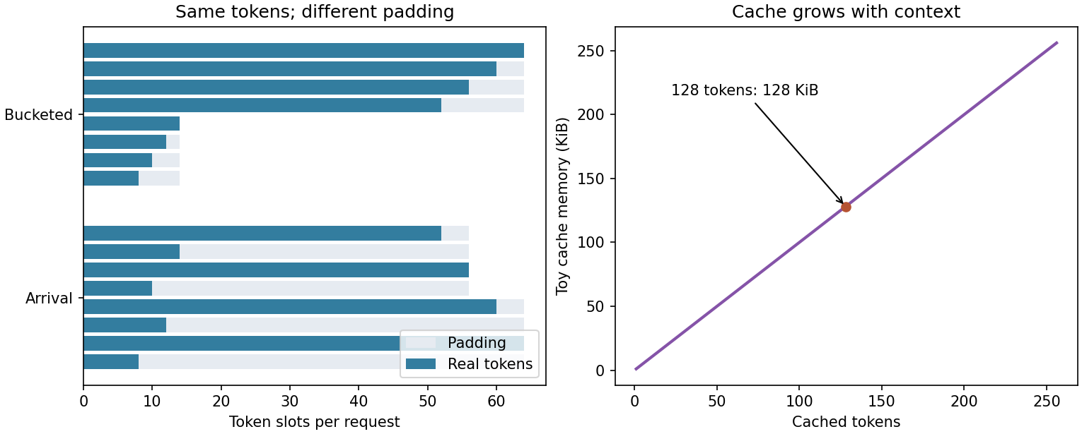
Autoregressive attention commonly caches prior keys and values to avoid recomputing them at every generated token. For a simple layout, the cache memory is approximately . Here is layer count, is the number of key/value heads, is head dimension, is cached token count, and is bytes per stored value. The factor two counts keys and values. Actual implementations add allocation and metadata costs and may use different layouts.
Separate time to first output token from time between subsequent tokens, total completion time and throughput under load. A short prompt with a long answer stresses a different stage from a long prompt with a short answer. Include preprocessing, waiting, validation and serialization in end-to-end measurements. Set a request-length limit, an output limit and a queue deadline based on measured workload behavior, and report what happens on timeout: a partial result, a retryable error or a reviewed fallback.
A reproducible serving contract
A model file alone cannot reproduce a prediction. Tokenization, normalization, evidence selection, decoding parameters, validation rules and output formatting all affect behavior. Hagiwara’s deployment chapter [1] supplies the practical reading for versioning, testing, train–serve differences and monitoring. For a learned generator, return the model version and the validated evidence IDs alongside the text, as the template function does, and store the preprocessing version and decoding configuration with the artifact. Logs should support diagnosis without unnecessarily retaining private source text.
Deploy a new version to a limited share of requests and compare it with a stable version using the same error categories. Check latency, completion rate and evidence correctness together. Keep rollback simple: a stored bundle should select the previous model, tokenizer, decoder settings and validation rules as one unit. Mixing an old model with a new tokenizer can create a failure that neither component exhibited alone.
Modern view
Plain version. Contemporary language modeling combines pretraining, adaptation, decoding, evaluation and system integration. Surveys are useful when they clarify these separate choices rather than compressing everything into one model ranking.
Zhao and colleagues’ survey [27], revised through 2026 and published in Frontiers of Computer Science, organizes large language models through pretraining, adaptation, utilization and capability evaluation. This framework helps distinguish more training data from instruction tuning or a different usage pattern. Chang and colleagues’ evaluation survey [28] separates questions about what to evaluate, where to evaluate and how to evaluate. Together they motivate a task-specific evaluation plan rather than relying on a single general score.
Li et al.’s pretrained-generation survey [29] organizes methods around input representation, architecture and optimization, and covers applications and evaluation. This taxonomy helps locate a change: retrieval alters available input evidence, an encoder–decoder changes conditional architecture, and adaptation changes parameters or training objectives. The survey predates some later systems, so use it for organization alongside newer evaluation and deployment evidence.
Ji et al.’s hallucination survey [20] and Schmidtova et al.’s survey of human evaluations of hallucination [30] approach the same problem from two sides. The first organizes definitions, metrics and mitigation across tasks; the second examines how studies define and assess hallucinations, and identifies inconsistent terminology and missing methodological reporting. Its practical lesson is to define source support, world knowledge and error severity separately, then publish annotation instructions and disagreement handling.
Gao and colleagues’ RAG survey [31] organizes retrieval-augmented systems into naive, advanced and modular paradigms, and separates context relevance, answer relevance and answer faithfulness. Stages interact: rewriting “What was the limit before the upgrade?” into “What is the temperature limit?” may improve topical retrieval while deleting the time constraint. Preserve the original query and compare the rewritten meaning, not only the retrieval score.
Kwon et al.’s PagedAttention work [32] studies key–value cache allocation and sharing in language-model serving. It addresses wasted memory and the batch sizes that memory permits, and supplies a concrete systems perspective on the cache calculation above. Its reported improvements belong to its workloads and comparisons; measure your own request lengths, concurrency and latency targets before adopting a serving design.
Open problems include contamination of evaluation sets, long-context robustness (a larger context window permits more input; it does not establish that all relevant parts are used reliably), multilingual and low-resource coverage, stable uncertainty, detection of unsupported claims without suppressing useful answers, and the relationship between instruction following and source-grounded correctness. Evaluation models can share errors with generators, especially when both rely on similar training data. A compact specialized model, or even a template, can be the better engineering choice when it satisfies the task with lower latency and simpler review.
Key takeaways
- A decoder-only Transformer factorizes text causally; shift targets explicitly and test that future tokens cannot change earlier logits.
- The GPT line kept one architecture and objective while scaling data, parameters and the way tasks are presented; scaling laws predict loss, not task behavior.
- Perplexity comparisons require compatible tokenization and evaluation positions, and say nothing directly about decoded outputs.
- Greedy and beam search optimize sequence probability; temperature reshapes the distribution; top-k and nucleus sampling cut its tail, with the nucleus adapting to the distribution’s shape.
- Generation needs a content contract: selection, planning and realization each fail differently, and extraction still needs mandatory-content checks.
- Overlap metrics, human review and model judges each have blind spots; validate them on the errors that matter, such as reversed negation.
- Retrieval supplies evidence, not authority; relevance, citation validity and claim support are separate conditions.
- Version the complete preprocessing–model–decoding–validation bundle, and treat instruction tuning and preference learning as distinct from factual support.
Exercises
- Remove the causal mask from the runnable causal model. Which assertion should fail, and why might training loss still look good?
Hint
The changed final token can become visible to earlier positions. Low loss can reward access to information unavailable during generation.
- Using the decoding code, find a temperature at which plain sampling puts more mass on the four tail tokens than top-k with ever can. Then construct a logit vector for which the nucleus with is larger than five tokens, and explain when each rule is the better choice.
Hint
Top-k with can keep at most one tail token. A flat logit vector makes the nucleus grow; a peaked one makes it shrink.
- Change the toy beam-search probabilities so beam search chooses a sentence that violates an externally supplied instruction. Add a constraint on permitted final sequences and compare its effect with widening the beam.
Hint
Probability search optimizes the distribution’s score. A permitted-sequence rule changes what outputs are admissible. Widening a beam need not repair a wrong probability model.
- Construct two candidate summaries: one with high word overlap but a wrong quantity, and another with lower overlap but correct meaning. Design an annotation form, and a model-judge protocol, that reveal this difference.
Hint
Ask reviewers to identify unsupported quantities and missing required facts before giving an overall usefulness judgment. Keep the source visible and system identity hidden; run the judge in both presentation orders.
- Construct one preference pair that rewards style but selects the less-supported response. Explain which additional evaluation would expose the problem, and compute the trainable parameter count of a rank-4 LoRA update for a 128-by-256 matrix.
Hint
Keep the evidence fixed and compare a confident answer that adds a fact with a qualified answer that preserves the source’s uncertainty. For LoRA, count the two factor matrices separately.
- Extend the report function with a timestamp and a target-language choice. Reject malformed inputs, preserve unknown status, attach evidence IDs and version the realization rules. Document the tests needed before replacing the template with a learned generator.
Hint
Do not infer an unrecorded timestamp or convert unknown into absent. Test preprocessing parity, number formatting, script requirements, long inputs, timeout behavior and the complete rollback bundle.
References
- Masato Hagiwara, Real-World Natural Language Processing: Practical Applications with Deep Learning, Chapters 5, 8, 9, 10 and 11, Manning, 2021. Publisher · Training practices · Deployment
- Susan McRoy, Principles of Natural Language Processing, open textbook, Chapters 6 and 9, 2021. Benchmark chapter · Generation chapter
- Ashish Vaswani et al., “Attention Is All You Need,” NeurIPS, 2017. Paper
- Alec Radford, Karthik Narasimhan, Tim Salimans and Ilya Sutskever, “Improving Language Understanding by Generative Pre-Training,” OpenAI technical report, 2018. Paper
- Alec Radford, Jeffrey Wu, Rewon Child, David Luan, Dario Amodei and Ilya Sutskever, “Language Models are Unsupervised Multitask Learners,” OpenAI technical report, 2019. Paper
- Tom B. Brown et al., “Language Models are Few-Shot Learners,” NeurIPS, 2020. Paper
- Jared Kaplan et al., “Scaling Laws for Neural Language Models,” arXiv:2001.08361, 2020. arXiv
- Jordan Hoffmann et al., “Training Compute-Optimal Large Language Models,” arXiv:2203.15556, 2022; published as “An empirical analysis of compute-optimal large language model training,” NeurIPS, 2022. arXiv
- Ilya Loshchilov and Frank Hutter, “Decoupled Weight Decay Regularization,” ICLR, 2019. Paper
- Dan Hendrycks and Kevin Gimpel, “Gaussian Error Linear Units (GELUs),” arXiv:1606.08415, 2016, revised 2023. Paper
- Jimmy Lei Ba, Jamie Ryan Kiros and Geoffrey E. Hinton, “Layer Normalization,” arXiv:1607.06450, 2016. Paper
- Ari Holtzman, Jan Buys, Li Du, Maxwell Forbes and Yejin Choi, “The Curious Case of Neural Text Degeneration,” ICLR, 2020. Paper
- Angela Fan, Mike Lewis and Yann Dauphin, “Hierarchical Neural Story Generation,” ACL, 2018. Paper
- Jade Goldstein and Jaime Carbonell, “Summarization: (1) Using MMR for Diversity-Based Reranking and (2) Evaluating Summaries,” TIPSTER Phase III Workshop, 1998. Paper
- Sam Wiseman, Stuart M. Shieber and Alexander M. Rush, “Challenges in Data-to-Document Generation,” EMNLP, 2017. Paper
- Ilya Sutskever, Oriol Vinyals and Quoc V. Le, “Sequence to Sequence Learning with Neural Networks,” NeurIPS, 2014. Paper
- Chin-Yew Lin, “ROUGE: A Package for Automatic Evaluation of Summaries,” Text Summarization Branches Out, 2004. Paper
- Lianmin Zheng et al., “Judging LLM-as-a-Judge with MT-Bench and Chatbot Arena,” NeurIPS Datasets and Benchmarks Track, 2023. Paper
- Peiyi Wang et al., “Large Language Models are not Fair Evaluators,” ACL, 2024. Paper
- Ziwei Ji et al., “Survey of Hallucination in Natural Language Generation,” ACM Computing Surveys 55, 2023. Survey
- Joshua Maynez, Shashi Narayan, Bernd Bohnet and Ryan McDonald, “On Faithfulness and Factuality in Abstractive Summarization,” ACL, 2020. Paper
- Patrick Lewis et al., “Retrieval-Augmented Generation for Knowledge-Intensive NLP Tasks,” NeurIPS, 2020. Paper
- OWASP GenAI Security Project contributors, “LLM01: Prompt Injection,” OWASP guidance, accessed 2026. Official guidance
- Edward J. Hu, Yelong Shen, Phillip Wallis, Zeyuan Allen-Zhu, Yuanzhi Li, Shean Wang, Lu Wang and Weizhu Chen, “LoRA: Low-Rank Adaptation of Large Language Models,” ICLR, 2022. Author publication page
- Long Ouyang et al., “Training language models to follow instructions with human feedback,” NeurIPS, 2022. Paper
- Rafael Rafailov, Archit Sharma, Eric Mitchell, Christopher D. Manning, Stefano Ermon and Chelsea Finn, “Direct Preference Optimization: Your Language Model is Secretly a Reward Model,” NeurIPS, 2023. Paper
- Wayne Xin Zhao et al., “A Survey of Large Language Models,” Frontiers of Computer Science, 2026. Updated survey
- Yupeng Chang et al., “A Survey on Evaluation of Large Language Models,” ACM Transactions on Intelligent Systems and Technology, 2024. Survey
- Junyi Li, Tianyi Tang, Wayne Xin Zhao, Jian-Yun Nie and Ji-Rong Wen, “Pre-Trained Language Models for Text Generation: A Survey,” ACM Computing Surveys, 2024. Publisher · Author manuscript
- Patricia Schmidtova et al., “Do My Eyes Deceive Me? A Survey of Human Evaluations of Hallucinations in NLG,” INLG, 2025. Survey
- Yunfan Gao, Yun Xiong, Xinyu Gao, Kangxiang Jia, Jinliu Pan, Yuxi Bi, Yi Dai, Jiawei Sun, Meng Wang and Haofen Wang, “Retrieval-Augmented Generation for Large Language Models: A Survey,” arXiv:2312.10997, revised 2024. Survey
- Woosuk Kwon et al., “Efficient Memory Management for Large Language Model Serving with PagedAttention,” SOSP, 2023. Conference · Paper
- Christopher D. Manning, Prabhakar Raghavan and Hinrich Schütze, Introduction to Information Retrieval, Chapters 6, 8 and 11, Cambridge University Press, 2008. Author-hosted book
- scikit-learn developers, “Text feature extraction,” scikit-learn documentation, accessed 2026. Documentation
- Vladimir Karpukhin, Barlas Oguz, Sewon Min, Patrick Lewis, Ledell Wu, Sergey Edunov, Danqi Chen and Wen-tau Yih, “Dense Passage Retrieval for Open-Domain Question Answering,” EMNLP, 2020. Paper
- Kalervo Järvelin and Jaana Kekäläinen, “Cumulated Gain-Based Evaluation of IR Techniques,” ACM Transactions on Information Systems 20(4), 422–446, 2002. Publisher
Check your understanding
This tutorial has 6 exercises. Can you solve them without opening the hints?
Go to the exercises ↑Next NLP 10 · Pretrained Models: BERT · 23 min