NLP 11 · Classification with BERT (Sentiment Analysis, Natural Language Inference)
Needs: NLP 10 · Pretrained Models: BERT
Navigate: this page and this track: Navigate: this page and this track
On this page
- What you’ll learn1 min
- The big picture1 min
- BERT applications: choose the output head4 min
- Single-text classification: sentiment analysis3 min
- Text pairs: natural language inference3 min
- Extractive QA as a pair task: answers need support5 min
- Benchmarks: GLUE and SuperGLUE1 min
- Fine-tuning practice3 min
- Evaluation: accuracy, macro-F1 and selective decisions2 min
- A runnable experiment: pretrain, then fine-tune3 min
- Modern view2 min
- Key takeaways1 min
- Exercises2 min
- Paper guides
- References
Natural Language Processing
Explore this chapter 2 interactive experiments
Change a right-context clue, hide it causally, then attach different output heads to the same small contextual vector.
What you’ll learn
- Choose the output head that matches the decision: one label, one label per token, or a span inside a passage.
- Fine-tune a pretrained encoder for sentiment analysis and for premise–hypothesis inference, and know what the standard datasets (SST, IMDB, SNLI, MultiNLI, SQuAD) actually contain.
- Recognize annotation artifacts, hypothesis-only baselines and challenge sets, and why a high in-distribution score can hide a shortcut.
- Set learning rate, epochs, warmup, class weights and decision thresholds deliberately, and know why fine-tuning can be unstable.
- Evaluate with accuracy, macro-F1, calibration and coverage, and separate relevant evidence from sufficient evidence.
- Run a tiny encoder that is pretrained from scratch with masked language modeling, then fine-tuned for synthetic sentiment and inference tasks on a CPU.
The big picture
NLP 10 built BERT: a bidirectional encoder pretrained by predicting masked tokens. Pretraining gives a representation function, not an application. A support team still has to say what “urgent” means, and an inference dataset still has to say when one sentence follows from another. This tutorial is about that second step: attaching a small output layer to the encoder, training both on labeled examples, and checking whether the result solves the intended task rather than a convenient imitation of it.
Two families of decisions dominate this chapter. Single-text classification assigns one label to one input: positive or negative sentiment, a topic, a ticket route. Text-pair classification labels the relationship between two inputs: does the hypothesis follow from the premise, contradict it, or neither? Extractive question answering sits next to them: instead of one label, the model chooses where an answer starts and ends inside a passage. All three reuse the same pretrained encoder; only the head and the training labels change [3].
Hagiwara’s Chapter 9 develops transfer learning with pretrained encoders for exactly these applications [1], and McRoy’s chapters on benchmark tasks and on information extraction and argumentation supply the linguistic side [2]. Throughout, keep one question in view: what evidence would convince a skeptic that the model learned the task, not the dataset?
BERT applications: choose the output head
Plain version. A task head turns the encoder’s token vectors into the output you need. Start by deciding whether the answer is one class, one label per token, or a span inside a passage.
| Application | Input | Supervised output |
|---|---|---|
| Sentiment, topic or support-ticket classification | One text | One category from the pooled [CLS] state |
| Entailment, paraphrase or query–document relevance | Two texts packed together | A relationship label or relevance score |
| Entity recognition or other token labeling | One tokenized text | A label at each supervised token position |
| Extractive question answering | Question and passage | Start/end positions in the passage |
| Semantic retrieval with Sentence-BERT | Texts encoded separately | Comparable vectors learned with a sentence-level objective |
Sequence and token tasks use the representations described in the BERT paper [3]; the original classification and span implementations make their output shapes explicit [4]. Sentence-BERT adds training for sentence comparisons [20]. The following formulas explain what those choices compute.
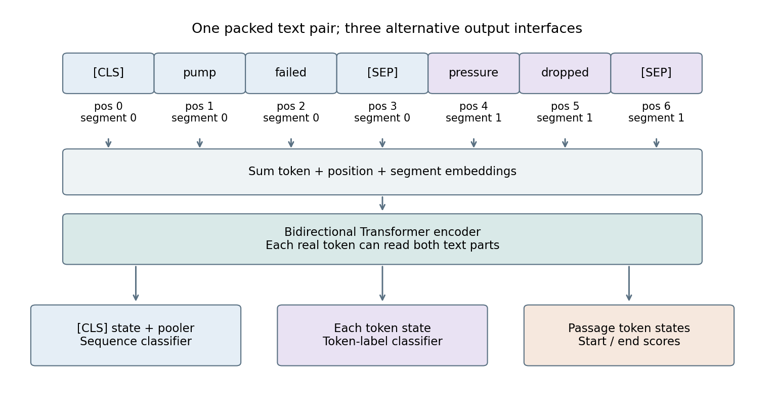
Sequence classification and text-pair decisions
For a classifier with classes, one common BERT interface is:
Here is the packed token sequence; is the first contextual row; and form the pooler; is its output; and form the classifier; and denotes class . Cross-entropy for the labeled category updates both head and encoder during end-to-end fine-tuning [4].
For “the pump failed,” a ticket classifier could predict an incident category. For a premise–hypothesis pair, the same output shape can represent entailment, contradiction or neither. The labels come from the task dataset, not from the next-sentence-prediction label vocabulary used in pretraining. Text-pair self-attention lets tokens in one text inspect the other before the final decision.
Token labeling
Attach a classifier to each contextual row:
Here is a token position and is the number of labels; and are shared across positions; is the token label; is its annotated value; and is the nonempty set of positions included in supervision. A device name split into multiple WordPieces requires a policy: supervise its first piece and ignore the others, or map the labels consistently across pieces. Exclude padding and special markers from . At inference, map predicted pieces back to word or character spans, as developed in NLP 06. Semantic role labeling in NLP 12 reuses the same head with a predicate marker.
Extractive question answering
Suppose the passage says “Pump B stopped at noon,” and the question asks “Which pump stopped?” Pack the question and passage together, encode them, then score possible answer boundaries:
Here are candidate start/end positions; are learned start/end vectors; are boundary scores; are their softmax distributions over allowed positions; and are annotated answer boundaries. Decode a valid span maximizing with and a declared maximum length [4]. Question positions and padding cannot be returned as passage answers. If a no-answer marker is included, train that option and select its decision threshold on development data.
The BERT paper introduces exactly two new vectors for this task, a start vector and an end vector, and computes each boundary probability as a dot product with the final token states followed by a softmax over passage positions [3]. Figure 2 shows why decoding must be joint rather than two independent argmaxes: the best start and the best end must form a legal span. In the synthetic scores, the highest-scoring legal span is “Pump B.”
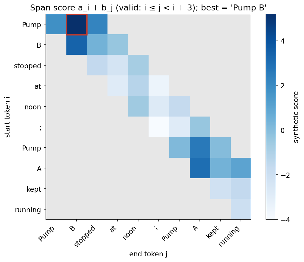
The returned answer is passage text such as “Pump B.” This setup does not generate an explanation or find a missing passage. Retrieval-augmented generation in NLP 09 handles finding passages; the sections on answerability below handle deciding whether a found passage is enough.
Retrieval: joint scoring or reusable vectors?
A joint BERT relevance model packs a query and candidate together, so the candidate’s representation depends on that query. It must run again for another pair. A sentence embedding model instead encodes documents separately and permits caching. Sentence-BERT trains this second interface with paired/triplet sentence objectives [20]. Raw pretrained [CLS] vectors or arbitrary mean pooling do not automatically provide a well-trained cosine retrieval space.
For a practical system, one design is to retrieve candidates using separately stored vectors, then jointly score a smaller set of query–candidate pairs. Evaluate the retrieval stage’s candidate recall separately from the final ranker. NLP 04 explains pooling and similarity; NLP 09 develops the full retrieval pipeline.
Single-text classification: sentiment analysis
Plain version. Sentiment analysis asks whether a text expresses a positive or negative opinion. It looks easy, but negation, contrast and mixed opinions mean that counting nice and nasty words is not enough.
Write the fine-tuning objective over labeled examples:
Here denotes the encoder parameters, initialized from pretraining; denotes the head parameters, initialized randomly; is the -th packed text; is its label; and is the classifier distribution defined above. Full fine-tuning updates both and . Freezing and training only is cheaper, but it can only reuse whatever distinctions the frozen features already make.
Two benchmark datasets and what they measure
The Stanford Sentiment Treebank (SST) contains 11,855 single sentences from movie reviews; the authors parsed them and had annotators label all 215,154 unique phrases in those parse trees [5]. Phrase-level labels let researchers study how sentiment composes: “not” combined with “good” is a phrase with its own label. The paper reports both fine-grained (five-class) and binary sentence-level results [5]. GLUE later adopted the two-way split as SST-2, listing about 67k training and 1.8k test examples and evaluating it with accuracy [14]. The original SST models were recursive networks over parse trees; ML 04 explains that architecture family.
The IMDB review dataset from Maas et al. contains 50,000 reviews divided evenly into 25,000 training and 25,000 test reviews, plus 50,000 unlabeled reviews; the labeled tasks are balanced two-class problems [6]. Its unit is a whole review, not a sentence. Reviews are often longer than a short encoder window, so a document classifier needs a stated truncation or chunking policy. Keep the head, the tail, or pool predictions over windows — each policy answers a slightly different question, because a review frequently changes tone near its end.
These two datasets illustrate a recurring issue: the unit of supervision defines the task. A sentence-level sentiment model trained on isolated opinions may fail on a whole conversation containing quotations, corrections and several speakers. If deployment includes previous turns, annotation and training should include the same permitted context. Conversely, giving annotators access to the final resolution while the model only sees the first message creates an impossible target. NLP 03 sets out this prediction contract in detail for count-based classifiers; the same contract applies after BERT.
What a contextual encoder adds, and what it does not
A bag-of-words classifier gives “good” the same weight in “the battery is good” and “the battery is not good.” A contextual encoder computes a different vector for “good” in each sentence, so the head can, in principle, learn the flip. NLP 03 runs a controlled negation test with count features and shows how sparse evidence leaves such a flip underdetermined. Context makes the distinction representable; the labeled data must still make it learnable. Phrase identity is also different from scope: distinguishing “not every repair succeeded” from “every repair failed” requires a compositional distinction that adjacent-word features do not supply, and that a fine-tuned encoder learns only if the training data contains it.
Treat sentiment labels as an annotation decision, too. A review can praise the screen and criticize the battery. Single-label sentiment forces such a review into one class; aspect-based sentiment instead assigns opinions to targets. Neither is “the true” task. Choose the one whose output the application consumes.
Text pairs: natural language inference
Plain version. A text can support a conclusion without proving that conclusion true in the world. Keep textual entailment and evidence quality separate.
Natural language inference (NLI) classifies a premise–hypothesis pair as entailment, contradiction or neutral under the annotation convention. If the premise is “Mina repaired a sensor,” the hypothesis “Someone repaired something” follows under an ordinary interpretation. “Mina repaired every sensor” does not follow, and “Mina repaired no sensor” conflicts with the premise.
For BERT, pack the pair as [CLS] premise [SEP] hypothesis [SEP] with segment IDs and , then apply the sequence head with :
Here is the premise token sequence, is the hypothesis token sequence, denote entailment, neutral and contradiction, and the other symbols are as in the sequence-classification head. Because self-attention crosses the [SEP] boundary, every hypothesis token can attend to every premise token in every layer. That joint encoding lets the decision depend on token-level comparisons between the two texts — and it is also the reason a pair model cannot cache one side.
SNLI and MultiNLI
The Stanford Natural Language Inference (SNLI) corpus contains 570,152 human-written sentence pairs labeled for entailment, contradiction and semantic independence (neutral) [7]. Annotators were shown an image caption as the premise and wrote hypotheses. The paper discusses a subtle labeling choice: whether two sentences should be assumed to describe the same event. Without that assumption, many apparent contradictions would be neutral. The corpus fixes one convention so that each pair receives one label [7]. That is exactly the kind of decision you must make — and document — for your own inference data.
MultiNLI extends the design to 433k examples from ten genres of written and spoken English. Only five genres appear in training, so the development and test sets have a matched section from the training genres and a mismatched section from the others [8]. The split turns domain shift into a measured quantity rather than an afterthought.
Annotation artifacts and hypothesis-only baselines
Crowd workers who are asked to write a contradiction often reach for the same tools: negation words, or a different activity. Gururangan et al. showed that a simple text classifier that sees only the hypothesis predicts the label for about 67% of SNLI and 53% of MultiNLI, and that phenomena such as negation and vagueness correlate strongly with particular classes [9]. Poliak et al. ran hypothesis-only baselines across ten NLI datasets and found that they significantly outperform the majority-class baseline on a number of them [10]. A model that ignores the premise cannot be performing inference, so its score measures dataset regularities.
McCoy, Pavlick and Linzen took the opposite direction: they built HANS, a controlled set where three syntactic heuristics — lexical overlap, subsequence and constituent — give the wrong answer, and found that models trained on MNLI, including BERT, perform very poorly on it [11]. Together these studies motivate two habits:
- Always run a partial-input baseline. If a hypothesis-only (or premise-only, or question-only) model does well, part of the benchmark score is not about the relationship you care about.
- Build challenge pairs that flip the cue. Hold the vocabulary fixed and change the one distinction that should matter: actor reversal, negation in the premise rather than the hypothesis, possibility versus assertion, allegation versus fact, one versus all.
An inference model predicts an annotation relationship. It does not independently verify the premise. If the premise itself is fabricated, an entailed hypothesis can also be fabricated. A retrieval-assisted application therefore needs both source selection and an answer-support check, which the question-answering sections below develop.
Argumentation mining can identify a claim, a proposed supporting statement and an expressed attack relation [2]. “The device is reliable because it passed one test” contains a recognizable argument structure. Identifying that structure does not establish that the test is representative or that the conclusion is valid. The application may store the stated reason while marking its evidential strength as unassessed.
Useful challenge pairs change one crucial distinction at a time. Fluent paraphrases are useful additional variation, but they should preserve the intended labels. A synthetic paraphrase that changes scope or removes attribution must receive a new annotation rather than inherit the original record automatically.
Optional: Sentence-BERT (in the Paper guides). Follow the original figure, objective, experimental comparisons and limitations.
Extractive QA as a pair task: answers need support
Plain version. SQuAD-style question answering asks the model to point at the answer inside a given passage. The harder practical question is whether the passage contains a supported answer at all.
The Stanford Question Answering Dataset (SQuAD) contains 107,785 question–answer pairs written by crowd workers on 536 Wikipedia articles; every answer is a span of the corresponding paragraph [12]. Its two metrics both ignore punctuation and the articles a, an and the: exact match is the percentage of predictions equal to one of the reference answers, and F1 measures token overlap between prediction and reference, averaged over questions [12]. Partial credit matters because annotators disagree mostly about non-essential words at span edges.
SQuAD 2.0 adds over 50,000 unanswerable questions written adversarially to look similar to answerable ones; a system must also decide when the paragraph supports no answer and abstain [13]. The BERT paper handles this by treating an unanswerable question as a span that starts and ends at [CLS]. At prediction time it compares the null score with the best non-null span score , and predicts an answer only when [3]. Here is a threshold selected on the development set to maximize F1. This one threshold converts a span model into a selective answerer.
A local evidence-backed answerer
We can demonstrate the answer contract without a trained span model. The answerer below handles one explicit question family and returns a source interval. It ranks four synthetic passages with TF–IDF, then answers only a narrow temperature-limit question for Pump A. It preserves one-character words so that the device identifier A remains a feature. The function is not a general classifier for question intent; its caller must route the declared question family to it.
Code · Python · 33 lines
import re
from sklearn.feature_extraction.text import TfidfVectorizer

corpus = {
    'temperature-v2': 'Pump A temperature limit is 80 C. This policy is current.',
    'shutdown-v1': 'Pump A shutdown follows a vibration alarm.',
    'label-v1': 'A technician replaced the cabinet label.',
    'sensor-v1': 'Sensor B reports humidity once per hour.',
}
ids = list(corpus)
vectorizer = TfidfVectorizer(ngram_range=(1, 2), token_pattern=r"(?u)\b\w+\b")
D = vectorizer.fit_transform([corpus[key] for key in ids])
def rank(query):
    score = (D @ vectorizer.transform([query]).T).toarray().ravel()
    order = sorted(range(len(ids)), key=lambda i: (-score[i], ids[i]))
    return [(ids[i], float(score[i])) for i in order]

def answer_temperature(query):
    if not re.search(r'\bpump\s+a\b', query, flags=re.I):
        return {'answer': None, 'reason': 'unsupported entity'}
    key, score = rank(query)[0]
    text = corpus[key]
    pattern = r'Pump A temperature limit is (\d+) C\.'
    match = re.search(pattern, text)
    if not match:
        return {'answer': None, 'reason': 'no matching evidence'}
    evidence = text[match.start():match.end()]
    result = {'answer': f'{match.group(1)} C', 'document': key,
              'start': match.start(), 'end': match.end(), 'evidence': evidence}
    assert text[result['start']:result['end']] == result['evidence']
    return result
print(answer_temperature('What is the Pump A temperature limit?'))
print(answer_temperature('What is the Pump Z temperature limit?'))
The supported Pump A answer returns 80 C, its document version and the character interval 0–33. A Pump Z question returns unsupported entity even though temperature-related passages exist. A span head trained on SQuAD-style data replaces the regular expression with learned boundary scores, but the surrounding contract — entity check, evidence interval, verified offsets, explicit abstention — should stay.
The explicit entity check prevents a high lexical score from transferring Pump A’s limit to an unsupported device. The evidence expression also requires the source to state the expected relation, not merely contain a number. A more flexible system needs a richer entity and relation check, including scope, units and applicable dates. Expand those capabilities with labeled tests rather than weakening the check until every question receives an answer.
The answerer searches only the top passage. It can therefore abstain when the correct evidence appears lower in the ranking. That limitation is intentional and visible. A later version could inspect several candidates under a fixed budget, while recording which candidate supplied the final answer. Measure the effect on both supported answers and false acceptance.
The function stores an evidence slice and verifies the offsets. This catches serialization mistakes, but not every semantic mistake. A quoted sentence can still describe the wrong entity, an outdated policy or a hypothetical case. Exact quotation is an important mechanical check; the support relation remains a separate part of the contract.
Relevance is not answerability
A passage can discuss the topic and still lack the requested fact. A system should have a meaningful way to return insufficient evidence.
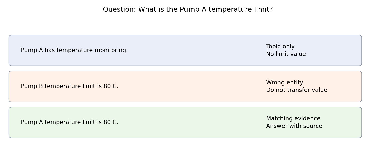
For a narrow question, define the required fields before evaluating a system. The temperature example needs device identity, a limit relation, a value and a unit. It may also need an effective date or operating condition. Missing any required field can make the available evidence insufficient even if the passage ranks first.
An abstention policy decides when to withhold an answer or ask for clarification. If confidence scores are used, select their threshold on development data with the intended costs of a wrong answer and unnecessary review — exactly the role of in the SQuAD 2.0 head. A raw similarity score is not a calibrated correctness probability. Its scale can change when the corpus, tokenizer or embedding model changes.
Report both coverage and quality among accepted answers:
Here is the number of evaluated questions; is the count receiving an answer; and counts accepted answers judged correct under the task contract. Accepted accuracy is undefined when no answer is accepted, so report that condition rather than presenting zero acceptance as a successful accuracy result.
Coverage must include questions without available answers. Otherwise a system that always answers can look good on a collection designed to contain an answer everywhere — the weakness SQuAD 2.0 was built to expose [13]. Include wrong entities, missing values, conflicting sources and unsupported time scopes. These cases test whether the model recognizes the limits of evidence instead of merely producing a likely span.
Diagnose failures with controlled substitutions
Replace one imperfect stage with a known-correct input to discover where the final answer fails. Keep these diagnostic results separate from end-to-end deployment scores.
First provide the answerer with the annotated supporting passage directly. If it still produces the wrong value, retrieval is not the immediate cause. Inspect entity matching, unit handling, scope and realization. If it succeeds with gold evidence but fails with retrieved evidence, inspect candidate recall and the selected passage order. This comparison localizes a bottleneck without pretending that perfect evidence will be available at deployment.
Next preserve the correct passage but add irrelevant or conflicting passages. A system that fails only after extra context arrives has a context-selection or evidence-integration problem. Vary one property at a time: a different device identifier, an obsolete version, a quoted allegation or an unsupported command. Label the intended behavior before running the experiment so the interpretation does not shift to excuse the output.
A supported answer requires a chain of successful decisions. For questions whose applicable evidence is in the corpus, write:
Here denotes probability, is the event that sufficient evidence survives retrieval, is the event that the evidence is interpreted correctly, and is the event that the output faithfully realizes the interpretation. The expression is the probability chain rule, not an independence assumption. Multiplying unrelated unconditional stage scores is not equivalent: reader accuracy on hand-picked easy passages may differ from reader accuracy on the retriever’s actual candidates.
This constructed evaluation makes the conditioning visible:
Code · Python · 12 lines
import numpy as np

retrieved = np.arange(100) < 80
interpreted = np.arange(100) < 72
realized = np.arange(100) < 68
r = retrieved.mean()
e = interpreted[retrieved].mean()
g = realized[retrieved & interpreted].mean()
complete = (retrieved & interpreted & realized).mean()
print('Conditional stage rates:', round(r, 3), round(e, 3), round(g, 3))
print('Complete supported answers:', round(complete, 3))
assert np.isclose(r * e * g, complete)
The rates are 0.8, 0.9 and 0.944, while complete success is 0.68. These are synthetic outcomes, not reported system performance. Individually respectable component results need not produce equally strong complete answers. Finally retain realistic query distributions: a diagnostic suite deliberately overrepresents difficult cases, while a representative held-out set estimates ordinary behavior. Report both with their purposes stated, and do not mix them into one aggregate number.
Benchmarks: GLUE and SuperGLUE
Plain version. A benchmark suite runs one pretrained model through many small tasks and summarizes them. It is good for comparing general-purpose encoders and poor at telling you whether your application works.
GLUE collects nine English understanding tasks — single-sentence tasks (acceptability and SST-2 sentiment), similarity and paraphrase tasks, and inference tasks including MNLI — together with a diagnostic dataset for specific linguistic phenomena and an online leaderboard [14]. None of its datasets was created from scratch for the benchmark, and some keep test labels private so that the leaderboard is used fairly [14]. Metrics differ by task: accuracy for SST-2, accuracy and F1 for paraphrase tasks, Pearson and Spearman correlations for sentence similarity, and the Matthews correlation coefficient for the unbalanced acceptability task [14]. The BERT paper reported its main transfer results on GLUE, SQuAD and a commonsense-inference set [3].
SuperGLUE keeps GLUE’s design — a leaderboard around eight tasks, a single summary number and analysis tools — but selects more difficult tasks, including yes/no question answering over passages and three-class entailment on embedded clauses [15].
Read a suite average carefully. It mixes tasks with different sizes, metrics and noise levels. A gain can come from one small task. It says nothing about artifacts unless partial-input baselines and challenge sets are reported, and nothing about your domain unless your domain is in it. Use suites to choose a starting checkpoint; use your own held-out data to choose a system.
Fine-tuning practice
Plain version. Fine-tuning is short supervised training starting from good weights. The main risks are a learning rate that destroys what pretraining learned, too few or too many updates, unlucky random seeds, and data whose class balance or label meaning differs from deployment.
Learning rate, epochs and schedule
The BERT authors kept dropout at 0.1 and reported that the following ranges worked well across their tasks: batch size 16 or 32; Adam learning rate , or ; and 2, 3 or 4 epochs [3]. They also observed that large datasets (100k+ labeled examples) were far less sensitive to these choices than small datasets [3]. The released classification script defaults to a learning rate of , three epochs, a maximum sequence length of 128 and a warmup proportion of 0.1 [4]. Its optimizer schedule is:
Here is the learning rate at update step ; is the configured peak rate; is the total number of training steps; and is the number of warmup steps, a fixed fraction of . The same implementation applies weight decay of 0.01 except to layer-normalization and bias parameters, and clips the global gradient norm at 1.0 [4]. AdamW-style decoupled weight decay is the standard name for this optimizer family [26].
Why so small a learning rate? Each update moves pretrained weights that encode useful distinctions. A rate suitable for training a randomly initialized network can erase them in a few hundred steps, after which the model is effectively learning from the small labeled set alone.
Instability and random restarts
For BERT-LARGE, the original authors found fine-tuning sometimes unstable on small datasets; they ran several random restarts, which changed data shuffling and classifier initialization while keeping the same pretrained checkpoint, and selected the best model on the development set [3]. Mosbach, Andriushchenko and Klakow analyzed this instability for BERT, RoBERTa and ALBERT on GLUE tasks. They attribute failed runs to optimization difficulties early in training, characterized by vanishing gradients, and the remaining variance to generalization differences between runs with almost identical training loss [16]. They did not observe the instability for BERT-BASE. Their guidelines for small datasets are to use small learning rates with Adam’s bias correction, and to train for considerably more iterations, close to zero training loss [16].
The practical lesson: report the spread over several seeds, not only the best seed, and select by development data only. A single lucky run is not a method.
Class imbalance
Real label distributions are rarely balanced. Class weighting changes how strongly each training example contributes:
Here is weighted cross-entropy, is training-example count, indexes examples, is the document, is its annotated class, is the chosen weight for that class and is the classifier distribution. The weighting policy changes the training objective; it does not manufacture missing linguistic variety.
Weighting, oversampling and threshold changes answer different problems. Weighting changes parameter learning. Oversampling changes the presentation frequency of examples, sometimes repeatedly exposing the same few minority examples. Thresholding changes the action policy after scores are computed. Hagiwara’s development discussion covers imbalance and training choices [1]. Evaluate any intervention on a realistic prevalence distribution rather than on an artificially balanced final test.
Calibration
A classifier can choose the right label while giving unreliable probabilities. Calibration asks whether predicted confidence agrees with observed correctness over comparable examples. A model can preserve its argmax decisions while changing confidence. Guo et al. study this distinction and post-training temperature scaling [17]:
Here is the logit vector, is a single temperature fit by minimizing negative log-likelihood on held-out development data, and is the rescaled distribution; for the expected calibration error , examples are grouped into confidence bins , is the number of examples, is the accuracy within bin and is its mean predicted confidence. Because dividing all logits by one positive number preserves their order, temperature scaling cannot change accuracy.
Desai and Durrett measured BERT and RoBERTa on NLI, paraphrase detection and commonsense reasoning. Used out of the box, the pretrained models were calibrated in-domain and had lower out-of-domain calibration error than the baselines they compared; temperature scaling reduced in-domain error further, and label smoothing helped out of domain [18]. Their result is a property of those tasks and models, not a guarantee for your fine-tuned checkpoint. Measure calibration on your own development data whenever probabilities drive an action such as abstention.
Evaluation: accuracy, macro-F1 and selective decisions
Plain version. Accuracy counts correct answers. Macro-F1 makes every class count equally, so a rare class cannot be ignored. Selective metrics ask how good the accepted answers are when the system may abstain.
For one class treated as positive:
Here is precision, is recall, counts true positives, counts false positives, counts false negatives and is their harmonic mean. A zero denominator requires an explicitly chosen convention. Macro F1 averages per-class F1 values equally; support-weighted averaging gives more influence to common classes. The metric documentation specifies these choices [19].
Accuracy is adequate for balanced tasks such as SST-2 or IMDB [6], [14]. For three-class NLI, report per-class F1 as well: a model can reach decent accuracy while confusing neutral with contradiction. For skewed tasks, macro-F1 or the Matthews correlation makes failures on a rare category visible, but neither encodes the actual cost of those failures. Missing an urgent ticket and misrouting a routine receipt can have different consequences. Write a cost policy separately rather than treating a convenient score as a complete utility measure.
For selective prediction:
Here is evaluated-example count, indicates acceptance of example , is its prediction, is its reference label, and is one when its condition holds and zero otherwise. Accepted risk is undefined when no example is accepted. A risk-versus-coverage curve describes the tradeoff over thresholds; choose the deployed threshold using validation rather than final test labels.
Then read the errors. Create an error table with text, gold label, predicted label, probability, language, length, source group and an analyst’s explanation. Useful error categories include annotation ambiguity, missing context, negation, unseen vocabulary, multi-topic input, quotation and genuinely out-of-scope text. These categories suggest different repairs. More training examples can help missing vocabulary; they cannot supply a conversation turn that is never available at prediction time. ML 11 covers the general evaluation and monitoring toolkit.
Keep model and preprocessing artifacts together. The tokenizer and vocabulary, maximum length and truncation policy, label order, calibration temperature and decision threshold are a single inference package. Reloading weights with another tokenizer silently changes meanings. Store a versioned label schema and a few deterministic contract examples with the package so that serving can check its assumptions.
A runnable experiment: pretrain, then fine-tune
Plain version. We pretrain a two-layer encoder from scratch with masked language modeling on a tiny unlabeled corpus, then fine-tune it for a sentiment task and an NLI task. The data are synthetic, so the experiment demonstrates mechanisms, not benchmark performance.
The design isolates three questions:
- Does pretraining transfer? The unlabeled corpus contains every adjective, each next to
loveorhate. The sentiment training set never containssuperborterrible; the test set contains only those two adjectives, with and withoutnot. A randomly initialized encoder has never seen them in any context. - Does a hypothesis-only baseline expose a shortcut? In the NLI training data,
notappears only in contradiction hypotheses — a deliberate annotation artifact. - Does a challenge set reveal it? The challenge set puts
notin an entailment (both sentences negated) and builds a contradiction whose hypothesis has nonot(the premise is negated instead).
The encoder follows the BERT recipe from NLP 10 in miniature: token + position + segment embeddings, layer normalization, two Transformer encoder blocks, 15% masked positions, and a pooled [CLS] head with a tanh layer for fine-tuning. It uses AdamW [26].
Code · Python · 109 lines
import itertools, random
import torch
from torch import nn
from torch.nn import functional as F
from sklearn.feature_extraction.text import CountVectorizer
from sklearn.linear_model import LogisticRegression
from sklearn.metrics import accuracy_score, f1_score

torch.manual_seed(0); random.seed(0); torch.set_num_threads(1)
POS, NEG = ['good', 'great', 'fine', 'superb'], ['bad', 'awful', 'poor', 'terrible']
ITEMS, NAMES = ['battery', 'screen', 'camera', 'speaker'], ['mina', 'ravi', 'lena']
VERBS = {'repaired': 'repair', 'cleaned': 'clean', 'tested': 'test'}
OBJS = ['the pump', 'the valve', 'the sensor']
words = set(' '.join(POS + NEG + ITEMS + NAMES + OBJS).split()) | set(VERBS) \
    | set(VERBS.values()) | set('the is not i love hate it someone did'.split())
vocab = ['[PAD]', '[CLS]', '[SEP]', '[MASK]'] + sorted(words)
idx, L, D = {w: i for i, w in enumerate(vocab)}, 16, 32

def batch(examples):                      # each example: (text,) or (text_a, text_b)
    ids, segs = [], []
    for ex in examples:
        toks, seg = ['[CLS]'], [0]
        for s, text in enumerate(ex):
            part = text.split() + ['[SEP]']
            toks += part; seg += [s] * len(part)
        ids.append([idx[t] for t in toks] + [0] * (L - len(toks)))
        segs.append(seg + [0] * (L - len(seg)))
    return torch.tensor(ids), torch.tensor(segs)

class TinyBERT(nn.Module):
    def __init__(self):
        super().__init__()
        self.tok, self.pos, self.seg = nn.Embedding(len(vocab), D), nn.Embedding(L, D), nn.Embedding(2, D)
        self.norm = nn.LayerNorm(D)
        block = nn.TransformerEncoderLayer(D, 2, 64, dropout=0.0, activation='gelu', batch_first=True)
        self.encoder = nn.TransformerEncoder(block, 2)
        self.mlm = nn.Linear(D, len(vocab))
    def forward(self, ids, seg):
        h = self.tok(ids) + self.pos(torch.arange(ids.shape[1])) + self.seg(seg)
        return self.encoder(self.norm(h), src_key_padding_mask=ids.eq(0))

# 1) Masked-LM pretraining on unlabeled text (no sentiment or NLI labels).
corpus = [(f'i love it the {i} is {a}',) for i in ITEMS for a in POS] \
    + [(f'i hate it the {i} is {a}',) for i in ITEMS for a in NEG] \
    + [(f'{n} {v} {o}',) for n in NAMES for v in VERBS for o in OBJS]
model = TinyBERT()
ids, seg = batch(corpus)
opt = torch.optim.AdamW(model.parameters(), lr=3e-3)
for step in range(400):
    pick = (torch.rand(ids.shape) < 0.15) & ids.gt(3)    # 15% of real tokens
    logits = model.mlm(model(ids.masked_fill(pick, idx['[MASK]']), seg))
    loss = F.cross_entropy(logits.flatten(0, 1), ids.masked_fill(~pick, -100).flatten())
    opt.zero_grad(); loss.backward(); opt.step()
print('final MLM loss:', round(loss.item(), 3))
pretrained_state = {k: v.clone() for k, v in model.state_dict().items()}

# 2) Fine-tune encoder + [CLS] head end to end.
def finetune(encoder, train, n_classes, epochs=60, lr=1e-3):
    torch.manual_seed(1)
    head = nn.Sequential(nn.Linear(D, D), nn.Tanh(), nn.Linear(D, n_classes))
    opt = torch.optim.AdamW([*encoder.parameters(), *head.parameters()], lr=lr)
    x, y = batch([ex for ex, _ in train]), torch.tensor([lab for _, lab in train])
    for _ in range(epochs):
        loss = F.cross_entropy(head(encoder(*x)[:, 0]), y)
        opt.zero_grad(); loss.backward(); opt.step()
    return lambda exs: head(encoder(*batch(exs))[:, 0]).argmax(-1).tolist()

def report(name, data, predict):
    gold = [lab for _, lab in data]
    with torch.no_grad():
        pred = predict([ex for ex, _ in data])
    print(f'{name:46s} acc={accuracy_score(gold, pred):.2f} '
          f'macro-F1={f1_score(gold, pred, average="macro"):.2f}')

# Task A: sentiment with negation. "superb" and "terrible" never get a label.
def review(item, adj, negated):
    return ((f'the {item} is {"not " * negated}{adj}',), int(adj in POS) ^ negated)
labeled = [a for a in POS + NEG if a not in ('superb', 'terrible')]
train_a = [review(i, a, n) for i in ITEMS for a in labeled for n in (0, 1)]
test_a = [review(i, a, n) for i in ITEMS for a in ('superb', 'terrible') for n in (0, 1)]
report('sentiment, pretrained encoder', test_a, finetune(model, train_a, 2))
report('sentiment, random-init encoder', test_a, finetune(TinyBERT(), train_a, 2))

# Task B: NLI (0 entailment, 1 neutral, 2 contradiction) with a negation shortcut.
def pair(n, v, o, kind):
    p, neg = f'{n} {v} {o}', f'{n} did not {VERBS[v]} {o}'
    other = list(VERBS)[(list(VERBS).index(v) + 1) % 3]
    return {'ent': ((p, f'someone {v} {o}'), 0), 'neu': ((p, f'{n} {other} {o}'), 1),
            'con': ((p, neg), 2),                   # training: "not" only in contradictions
            'neg-ent': ((neg, neg), 0),             # challenge: "not" in an entailment
            'neg-con': ((neg, p), 2)}[kind]         # challenge: contradiction without "not"
triples = list(itertools.product(NAMES, VERBS, OBJS)); random.shuffle(triples)
train_b = [pair(*t, k) for t in triples[:18] for k in ('ent', 'neu', 'con')]
test_b = [pair(*t, k) for t in triples[18:] for k in ('ent', 'neu', 'con')]
challenge = [pair(*t, k) for t in triples[18:] for k in ('neg-ent', 'neu', 'neg-con')]

vec = CountVectorizer(token_pattern=r'\S+').fit([ex[1] for ex, _ in train_b])
hyp_only = LogisticRegression(C=10, max_iter=1000).fit(
    vec.transform([ex[1] for ex, _ in train_b]), [lab for _, lab in train_b])
hyp_predict = lambda exs: hyp_only.predict(vec.transform([ex[1] for ex in exs])).tolist()
model.load_state_dict(pretrained_state)
pair_predict = finetune(model, train_b, 3)
for split, data in [('in-distribution', test_b), ('challenge', challenge)]:
    report(f'NLI {split}, hypothesis-only', data, hyp_predict)
    report(f'NLI {split}, pair encoder', data, pair_predict)
counter = [pair(*t, k) for t in triples[:18] for k in ('neg-ent', 'neg-con')]
model.load_state_dict(pretrained_state)
report('NLI challenge, pair encoder + counterexamples', challenge,
       finetune(model, train_b + counter, 3))
The run takes a few seconds on one CPU thread and prints:
Code · 8 lines
final MLM loss: 0.621
sentiment, pretrained encoder                  acc=1.00 macro-F1=1.00
sentiment, random-init encoder                 acc=0.25 macro-F1=0.20
NLI in-distribution, hypothesis-only           acc=1.00 macro-F1=1.00
NLI in-distribution, pair encoder              acc=1.00 macro-F1=1.00
NLI challenge, hypothesis-only                 acc=0.33 macro-F1=0.22
NLI challenge, pair encoder                    acc=0.67 macro-F1=0.56
NLI challenge, pair encoder + counterexamples  acc=1.00 macro-F1=1.00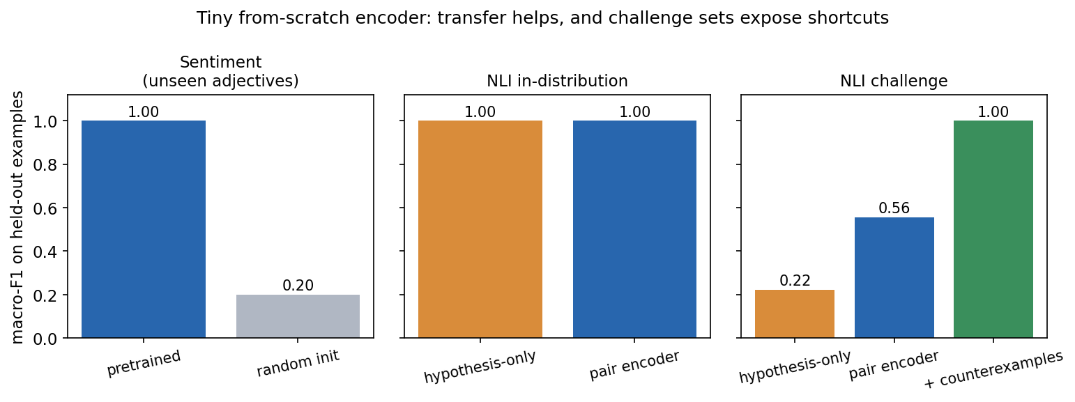
Transfer. The pretrained encoder labels all sixteen test sentences correctly, including the negated ones, although superb and terrible never appeared with a label. During pretraining they shared contexts with love and hate respectively, so their representations already sat near the labeled adjectives of the same polarity. The randomly initialized encoder has only random embeddings for the two words, and the fine-tuning set gives it nothing to connect them to the labels. This is the BERT argument at toy scale: unlabeled text can supply distinctions that a small labeled set cannot. It also shows the dependency: transfer worked because the unlabeled corpus contained the relevant co-occurrence. Pretraining on unrelated text would not help.
Shortcut. In distribution, the hypothesis-only logistic regression is perfect. That is the warning sign: a model that never reads the premise cannot be doing inference, so the test set does not require inference. The fine-tuned pair encoder is also perfect in distribution, which on its own tells us nothing about what it uses.
Challenge. On the challenge set, the hypothesis-only baseline drops to chance-level accuracy. Inspecting the predictions shows that the pair encoder classifies every negated contradiction and every neutral pair correctly, but labels all nine doubly negated entailments as contradictions — it has partly learned “not in the hypothesis means contradiction.” Adding eighteen counterexamples of the two challenge types (built from the training names, verbs and objects) fixes the challenge set. Be careful with that last line: the counterexamples share templates with the challenge set, so a perfect score shows that the model can learn the distinction once the data demands it, not that it would generalize to a new kind of shortcut.
Everything here is deliberately small: a 40-word vocabulary, sentences of at most a dozen tokens, one seed. Across the four seeds we tried, the qualitative pattern is the same, but the exact random-init and challenge numbers move. Exercise 5 asks you to measure that spread.
Modern view
Surveys and their maps. Minaee et al.’s ACM Computing Surveys review covers more than 150 deep-learning text classifiers and more than 40 datasets across sentiment analysis, news categorization, question answering and natural language inference [21]. It groups models by architecture — feed-forward, recurrent, convolutional, capsule, attention, memory-augmented, graph, Siamese, hybrid, and Transformer-based pretrained language models — and its central takeaway is that pretrained language models fine-tuned with task labels had set new states of the art on many text classification tasks. Chang et al.’s evaluation survey separates what to evaluate, where (which benchmarks) and how (automatic, human, protocols) [24], and Zhao et al.’s survey places classification inside the broader workflow of pretraining, adaptation, utilization and capability evaluation [25]. Read together, they argue for task-specific evaluation plans rather than one leaderboard number.
Encoders in the LLM era (2023–2026). Large decoder-only models can classify by prompting, without task-specific weights. Zhang et al. evaluated LLMs on 13 sentiment tasks across 26 datasets against small models trained on domain data. LLMs performed satisfactorily on simpler tasks but lagged on tasks that need structured sentiment information or a deeper understanding of specific phenomena, while clearly outperforming the small models in few-shot settings [22]. The practical reading: prompting is a strong option when labels are scarce, and a fine-tuned encoder remains competitive when labeled data exist and latency matters. Encoders themselves are still evolving. ModernBERT, published at ACL 2025, brings recent architecture and training optimizations to encoder-only models, trains on 2 trillion tokens with a native 8,192-token sequence length, and reports strong results across classification and retrieval evaluations along with speed and memory efficiency [23]. The fine-tuning interface in this chapter — a head on [CLS] or on token states — carries over unchanged.
What did not change. Annotation artifacts [9], [10] and heuristic shortcuts [11] are properties of datasets and training signals, not of one architecture. A larger or newer model can still learn them, and a prompted model can bring its own. Partial-input baselines, challenge sets, calibration checks [18] and abstention policies [13] remain the tools for finding out.
Open problems. Robustness under domain shift (the MultiNLI matched/mismatched split [8] is an early, narrow version), calibrated abstention for long and multi-passage inputs, multilingual and code-switched sentiment, labels that change with policy, and evaluation sets that leak into pretraining corpora. Each is easier to study with a small, transparent baseline next to the large model.
Key takeaways
- The encoder is shared; the head and the labels define the task. Choose sequence, token or span output first.
- Pair tasks pack both texts into one sequence so that attention can compare them token by token; the price is that neither side can be cached.
- The unit of supervision — sentence, review, conversation — is part of the task definition.
- A hypothesis-only (partial-input) baseline that scores well means the benchmark does not fully require the relationship you care about.
- Challenge sets that flip one cue at a time reveal shortcuts that in-distribution accuracy hides.
- Fine-tune with small learning rates, warmup and decay; report variance over seeds and select on development data.
- Evaluate decisions (accuracy, macro-F1), probabilities (calibration) and abstention (coverage, accepted risk) as separate properties.
- Relevance is not answerability: a span answer needs a supporting passage and an explicit way to say “not stated.”
Exercises
- Truncation policy. You must classify reviews that are often longer than the encoder window. Compare keeping the first tokens, the last tokens, and averaging predictions over overlapping windows. Which reviews would each policy misjudge?
Hint
Write three short synthetic reviews whose verdict appears at the start, at the end, and is reversed halfway (“at first I liked it … but”). Decide which label the annotation guideline intends before choosing a policy.
- A partial-input audit. For the NLI data in the experiment, train a premise-only baseline as well. Predict its accuracy before running it, then explain the result.
Hint
In the training templates, every premise appears with all three labels. A premise-only model can do no better than the majority class; compare that with the hypothesis-only result.
- SQuAD 2.0 threshold. Given development-set scores and for answerable and unanswerable questions, describe how to choose , and what happens to coverage and accepted accuracy as grows.
Hint
Sweep over the observed score differences . A larger answers fewer questions. Plot coverage against accepted accuracy, then pick the point that matches the stated cost of a wrong answer.
- Calibration. Add temperature scaling to the experiment’s sentiment classifier: fit one temperature on a held-out split by minimizing negative log-likelihood. Show that accuracy cannot change and measure how the mean confidence moves.
Hint
Dividing logits by a positive scalar preserves their order. Optimize instead of to keep the temperature positive.
- Seed variance. Run the experiment with five seeds for pretraining and fine-tuning. Report the mean and range of each line, and decide which conclusions survive.
Hint
Change both torch.manual_seed calls. Separate claims about direction (pretrained better than random-init; challenge lower than in-distribution) from claims about exact values.
- Inference challenge pairs. Create six NLI pairs that separately test role reversal, negation in the premise, modality, attribution, quantifier scope and time. Write the intended label and the assumptions before evaluating any model.
Hint
Preserve neutral as an option when the premise supplies too little information. For attribution, compare “Mina said the pump failed” with “The pump failed.”
References
- Masato Hagiwara, Real-World Natural Language Processing: Practical Applications with Deep Learning, Chapters 9–11, Manning, 2021. Publisher
- Susan McRoy, Principles of Natural Language Processing, Chapters 6 and 8, open textbook, 2021. Open textbook
- Jacob Devlin, Ming-Wei Chang, Kenton Lee and Kristina Toutanova, “BERT: Pre-training of Deep Bidirectional Transformers for Language Understanding,” NAACL-HLT, 2019. Paper
- Google Research, BERT: original implementation, software, 2018. Classification, Question answering, Optimizer
- Richard Socher, Alex Perelygin, Jean Wu, Jason Chuang, Christopher D. Manning, Andrew Ng and Christopher Potts, “Recursive Deep Models for Semantic Compositionality Over a Sentiment Treebank,” EMNLP, 2013. Paper
- Andrew L. Maas, Raymond E. Daly, Peter T. Pham, Dan Huang, Andrew Y. Ng and Christopher Potts, “Learning Word Vectors for Sentiment Analysis,” ACL-HLT, 2011. Paper
- Samuel R. Bowman, Gabor Angeli, Christopher Potts and Christopher D. Manning, “A large annotated corpus for learning natural language inference,” EMNLP, 2015. Paper
- Adina Williams, Nikita Nangia and Samuel R. Bowman, “A Broad-Coverage Challenge Corpus for Sentence Understanding through Inference,” NAACL-HLT, 2018. Paper
- Suchin Gururangan, Swabha Swayamdipta, Omer Levy, Roy Schwartz, Samuel R. Bowman and Noah A. Smith, “Annotation Artifacts in Natural Language Inference Data,” NAACL-HLT, 2018. Paper
- Adam Poliak, Jason Naradowsky, Aparajita Haldar, Rachel Rudinger and Benjamin Van Durme, “Hypothesis Only Baselines in Natural Language Inference,” *SEM, 2018. Paper
- R. Thomas McCoy, Ellie Pavlick and Tal Linzen, “Right for the Wrong Reasons: Diagnosing Syntactic Heuristics in Natural Language Inference,” ACL, 2019. Paper
- Pranav Rajpurkar, Jian Zhang, Konstantin Lopyrev and Percy Liang, “SQuAD: 100,000+ Questions for Machine Comprehension of Text,” EMNLP, 2016. Paper
- Pranav Rajpurkar, Robin Jia and Percy Liang, “Know What You Don’t Know: Unanswerable Questions for SQuAD,” ACL, 2018. Paper
- Alex Wang, Amanpreet Singh, Julian Michael, Felix Hill, Omer Levy and Samuel R. Bowman, “GLUE: A Multi-Task Benchmark and Analysis Platform for Natural Language Understanding,” ICLR, 2019. Paper
- Alex Wang, Yada Pruksachatkun, Nikita Nangia, Amanpreet Singh, Julian Michael, Felix Hill, Omer Levy and Samuel R. Bowman, “SuperGLUE: A Stickier Benchmark for General-Purpose Language Understanding Systems,” NeurIPS, 2019. Paper
- Marius Mosbach, Maksym Andriushchenko and Dietrich Klakow, “On the Stability of Fine-tuning BERT: Misconceptions, Explanations, and Strong Baselines,” ICLR, 2021. Paper
- Chuan Guo, Geoff Pleiss, Yu Sun and Kilian Q. Weinberger, “On Calibration of Modern Neural Networks,” ICML, 2017. Paper
- Shrey Desai and Greg Durrett, “Calibration of Pre-trained Transformers,” EMNLP, 2020. Paper
- scikit-learn developers, “Classification metrics,” scikit-learn documentation, current online edition. Documentation
- Nils Reimers and Iryna Gurevych, “Sentence-BERT: Sentence Embeddings using Siamese BERT-Networks,” EMNLP-IJCNLP, 2019. Paper
- Shervin Minaee, Nal Kalchbrenner, Erik Cambria, Narjes Nikzad, Meysam Chenaghlu and Jianfeng Gao, “Deep Learning–based Text Classification: A Comprehensive Review,” ACM Computing Surveys 54(3), 2021. Survey
- Wenxuan Zhang, Yue Deng, Bing Liu, Sinno Jialin Pan and Lidong Bing, “Sentiment Analysis in the Era of Large Language Models: A Reality Check,” Findings of NAACL, 2024. Paper
- Benjamin Warner, Antoine Chaffin, Benjamin Clavié, Orion Weller, Oskar Hallström, Said Taghadouini et al., “Smarter, Better, Faster, Longer: A Modern Bidirectional Encoder for Fast, Memory Efficient, and Long Context Finetuning and Inference,” ACL, 2025. Paper
- Yupeng Chang et al., “A Survey on Evaluation of Large Language Models,” ACM Transactions on Intelligent Systems and Technology, 2024. Survey
- Wayne Xin Zhao et al., “A Survey of Large Language Models,” Frontiers of Computer Science, 2026. Updated survey
- Ilya Loshchilov and Frank Hutter, “Decoupled Weight Decay Regularization,” ICLR, 2019. Paper
Check your understanding
This tutorial has 6 exercises. Can you solve them without opening the hints?
Go to the exercises ↑Next NLP 12 · Syntactic and Semantic Tasks · 38 min