NLP 02 · Linguistic Essentials
Needs: NLP 01 · Introduction to Natural Language Processing
Navigate: this page and this track: Navigate: this page and this track
On this page
- What you’ll learn1 min
- The big picture1 min
- 1. Language, modality and units2 min
- 2. Morphology: structure inside words5 min
- 3. Tokens and subwords4 min
- 4. Parts of speech2 min
- 5. Syntax: order, grouping and grammatical relations3 min
- 6. Semantics: meanings and truth conditions4 min
- 7. Pragmatics: interpretation in a situation3 min
- 8. Discourse: meaning across sentences and turns1 min
- 9. Corpora, annotation and Zipf’s law3 min
- 10. Linguistic diversity and model assumptions2 min
- 11. A complete worked reading2 min
- Modern view2 min
- Key takeaways1 min
- Exercises1 min
- Paper guides
- References
Natural Language Processing
Explore this chapter 2 interactive experiments
Change a small reading relation and evaluate two quantifier orders exactly.
What you’ll learn
- Distinguish language from its spoken, signed and written forms, and distinguish linguistic units from computational tokens.
- Analyze word structure, compare stemming with lemmatization, and enumerate ambiguous Chinese segmentations.
- Train a small BPE tokenizer and relate it to WordPiece, the unigram model and SentencePiece.
- Use Universal Dependencies part-of-speech tags and explain why grouping, grammatical relations and agreement carry information that word counts omit.
- Work out lexical meaning, composition, negation and quantifier scope, and separate assertion, presupposition, implicature and discourse relations.
- Read corpora and annotations critically: agreement between annotators, Zipf’s law and the long tail of rare words.
The big picture
Language lets people describe situations, ask questions, coordinate action and change what others know. The visible sentence is only part of that activity. Its internal structure constrains interpretation; speakers also rely on shared objects, earlier conversation and expectations about why someone spoke.
Consider “The technician inspected the panel with the camera.” Did the technician use a camera, or inspect a panel that had a camera attached? Knowing every dictionary entry does not settle the question. Consider “Can you inspect it tomorrow?” Now the object, reference date and intended request depend on context. A useful analysis identifies these alternatives before choosing a representation or label.
This tutorial supplies the language foundation for the practical route in Hagiwara’s Real-World Natural Language Processing [1] and the symbolic and computational route in McRoy’s Principles of Natural Language Processing [2]. Essentials of Linguistics, an open textbook, supplies additional linguistic grounding [3]. The examples here are original. NLP 01 introduced the task-to-evaluation pipeline; this tutorial supplies the units and structures that pipeline must preserve. Later tutorials turn them into models: NLP 06 tags parts of speech and entities, and NLP 12 parses sentences, labels semantic roles and resolves coreference. These levels interact rather than forming a compulsory sequence of separate software modules.
1. Language, modality and units
Plain version. Speech, signing and writing are different ways of expressing language, and each records different information. A computer’s “token” is yet another unit, chosen for processing.
Language is a system of structured expression and interpretation. Speech and writing are ways to express it; they are not interchangeable containers. Signed languages use systematic visual-manual expression, and tactile signing provides another modality [4]. A written transcript preserves selected information from an interaction, while leaving out timing, gaze, gesture and much of its physical setting.
Sounds and written symbols answer different questions
Phonetics studies the physical production and perception of speech sounds. Phonology studies their patterning within a language. A phoneme is a contrastive sound unit in a particular linguistic system; different physical realizations can belong to the same phoneme [5]. A grapheme is a unit of a writing system. These units need not map one to one.
English “ship” has four letters, yet its initial “sh” represents one consonant sound. Conversely, a letter can contribute differently in different words. Counting letters therefore cannot directly answer a question about sound structure. A speech application and a text application may need different annotations even when their users intend the same words.
Tone and intonation also differ [6]. Mandarin mā, má, mǎ and mà distinguish the ordinary written words 媽, 麻, 馬 and 罵. Their tone patterns contribute to lexical contrasts. The broader contour of an utterance can also convey questioning or emphasis. In English, “Really.” and “Really?” suggest different interpretations in writing, but punctuation only approximates how an actual speaker expresses disbelief, curiosity or confirmation. The written question mark does not recover the original voice.
Characters, words and tokens
A word form is a particular realized form; a lexeme groups related forms as one vocabulary item. For a simplified analysis, “repair,” “repairs” and “repaired” are forms of the verb lexeme REPAIR. A lemma is a chosen citation form used to index that item. Lemmatization is thus an annotation decision, not a claim that the surface forms are interchangeable in a sentence [2, 3].
The distinctions matter in “The technician repairs cameras” versus “The technician repaired cameras.” Grouping both verbs under REPAIR helps search for the activity, but discarding the forms loses a present-versus-past contrast. An application can preserve both the original span and its lemma rather than deciding that one representation must replace the other.
A computational token is an input unit selected by a processing procedure. It might be a word, part of a word, punctuation or a character sequence. Its boundaries need not coincide with phonemes, morphemes or lexemes. Likewise, a Chinese character can participate in a multi-character word: the written sequence 相機 denotes a camera. A character-based system receives two units where a word-oriented analysis may use one. Neither count independently defines the number of meanings in the phrase.
2. Morphology: structure inside words
Plain version. Words have parts. Some parts carry vocabulary meaning, others carry grammar such as tense or number, and the way the parts are grouped can change the meaning.
Word structure can convey both vocabulary meaning and grammatical information. Morphology studies that structure; a morpheme is a minimal recurring pairing of form with meaning or grammatical function [7]. “Minimal” does not mean “one letter,” and a meaningful element need not stand alone. Morphological evidence such as a plural ending, tense marker or derivational prefix is useful, but not every language expresses these properties with the same pieces or word boundaries.
Inflection, derivation and productive formation
An inflectional contrast changes a word’s grammatical realization, as in repair/repaired. A derivational process can create a new vocabulary item, as in repair/repairable. A compound combines bases, as in camera mount [3, 7]. These are analytical distinctions: identifying an ending’s spelling is not enough to decide its function.
Compare “repairs” in “She repairs the camera” and “The repairs took a day.” In the first sentence, it is a finite verb form; in the second, a plural noun. A rule that strips every final “s” loses both grammatical category and the reason for the ending. It would also mishandle irregular pairs such as mouse/mice. The task is to explain recurring form–function patterns, with exceptions represented explicitly.
Productivity means that a pattern can support new combinations, rather than merely describing a memorized list. If a workshop introduces a new “sensor cradle,” listeners can interpret the compound from familiar pieces and the setting. Yet composition does not specify every detail: the cradle might hold a sensor during assembly, transport or operation. Word formation can supply a general relation while context supplies its exact instance.
Chinese also has internal word structure and productive combinations. In 三台相機, 三 expresses the count, 台 is a classifier associated with the counted object, and 相機 names the object. English “three cameras” places plural marking on the noun in this example. The contrast identifies different grammatical choices; it does not establish that Chinese words lack structure or that English nouns always carry an explicit count.
Stemming versus lemmatization
Plain version. A stemmer chops endings off by rule; a lemmatizer looks up the dictionary form, using the word’s grammatical category. The stemmer is cheap and crude; the lemmatizer needs more knowledge and makes fewer blunders.
A stemmer maps word forms to a shared string, the stem, by rewriting suffixes. Porter’s algorithm is the classic English example: it applies ordered groups of suffix rules, each guarded by a condition on the remaining stem, and was designed to improve information retrieval by grouping related terms [16]. The stem need not be a real word; it only has to be consistent. A lemmatizer returns the lemma, which requires a lexicon and usually the part of speech: “saw” is the lemma of a noun but a form of SEE as a verb.
The toy stripper below uses four ordered rules and a minimum-stem-length guard, in the spirit of (but far simpler than) Porter’s algorithm. The lookup table stands in for a dictionary.
Code · Python · 21 lines
# A toy suffix stripper (a few Porter-style rules) versus a lookup lemmatizer.
RULES = [("ies", "y"), ("ing", ""), ("ed", ""), ("s", "")]   # tried in order; first match wins

def stem(word):
    for suffix, replacement in RULES:
        if word.endswith(suffix) and len(word) - len(suffix) >= 3:
            return word[: -len(suffix)] + replacement
    return word

# A lemmatizer needs the part of speech; this tiny table stands in for a dictionary.
LEMMAS = {("repairs", "VERB"): "repair", ("repairs", "NOUN"): "repair",
          ("repaired", "VERB"): "repair", ("mice", "NOUN"): "mouse",
          ("was", "AUX"): "be", ("batteries", "NOUN"): "battery",
          ("news", "NOUN"): "news", ("this", "DET"): "this"}

def lemmatize(word, pos):
    return LEMMAS.get((word, pos), word)

for word, pos in [("repairs", "VERB"), ("repaired", "VERB"), ("batteries", "NOUN"),
                  ("mice", "NOUN"), ("was", "AUX"), ("news", "NOUN"), ("this", "DET")]:
    print(f"{word:10s} stem={stem(word):9s} lemma={lemmatize(word, pos)}")
The stripper handles the regular forms (repairs, repaired, batteries all reach a sensible stem) but returns mice and was unchanged and damages news → new and this → thi. The first two failures are irregular morphology; the last two are over-stemming, where an ending that only looks like a suffix is removed. The lemmatizer gets all seven right, but only because its table already contains them; an unseen word passes through unchanged. Neither tool decides the grammatical category: the caller supplied VERB or NOUN, which is the job of the tagger in NLP 06.
Which one to use depends on the task. For search, merging repairs and repaired can raise recall even if a few unrelated words collide. For a status extractor, the tense the stemmer throws away may be exactly the answer. Modern neural pipelines rarely stem their input; they keep the original form and let subword tokens and context carry the morphology, which is one reason the next section matters.
The same pieces can combine in different orders
An invented description “an unsealable case” permits two useful structural analyses:
un + (seal + able): a case that cannot be sealed.(un + seal) + able: a case that can be unsealed.
The first treats “un” as negating an adjective; the second treats it as reversing the sealing action before “able” forms an adjective. The readings have opposite practical implications. Their availability and naturalness depend on context, so the example demonstrates possible analyses rather than claiming that every speaker assigns both equally often.
A bag of these pieces is identical in both analyses. What changes is the intermediate grouping and the kind of object each operation combines with. The same problem will reappear in sentence attachment and logical scope: a representation must retain structure if the distinction matters to the task.
Chinese segmentation is an interpretation problem
Written Chinese does not mark word boundaries with spaces. The original string 學生會說話 supports “學生 / 會 / 說話” (“students can speak”) and “學生會 / 說話” (“the student council speaks”). The first reading treats 會 as expressing ability. The second treats 學生會 as a compound noun. Spaces inserted after processing therefore record an analysis; the unspaced string does not supply them directly.
The following program enumerates paths through a small, explicit lexicon. It is not a general Chinese segmenter. It shows why choosing the longest matching entry cannot establish the speaker’s intended reading.
Code · Python · 19 lines
from functools import lru_cache

text = "學生會說話"
lexicon = ("學生", "學生會", "會", "說話")

@lru_cache(None)
def segment(start):
    if start == len(text):
        return ((),)
    paths = []
    for word in lexicon:
        if text.startswith(word, start):
            for rest in segment(start + len(word)):
                paths.append((word,) + rest)
    return tuple(paths)

for path in segment(0):
    print(" / ".join(path))
assert len(segment(0)) == 2
The two printed paths are the readings above. Every recursive step consumes a known word, and the base case accepts only complete coverage. Enlarging the lexicon may add alternatives; it does not add evidence about a particular conversation. A syntax analysis, the surrounding sentence or knowledge that the message concerns a council meeting could favor one path.
Even the gold standard is a choice. The Second International Chinese Word Segmentation Bakeoff evaluated systems on four corpora, two in Traditional characters (from Academia Sinica in Taiwan and City University of Hong Kong) and two in Simplified characters (from Peking University and Microsoft Research), and each provider segmented its data under its own standard [27]. A system can therefore be “wrong” on one corpus and “right” on another for the same split. Report which segmentation standard your labels follow.
3. Tokens and subwords
Plain version. A model needs a fixed list of units. Whole words leave too many unknown words; single characters make sequences long. Subword methods learn a middle ground from data: frequent strings become single tokens, rare ones are spelled out from smaller pieces.
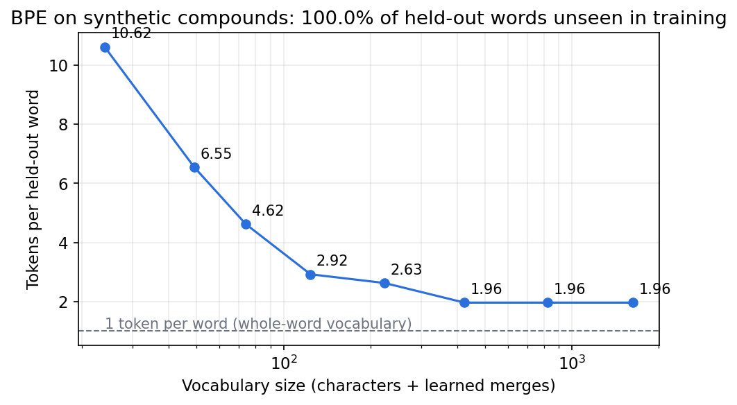
NLP 01 defined the unknown-token rate and showed why mapping every unseen word to one marker loses distinctions. A character vocabulary reduces whole-word unknowns if the necessary characters are covered, at the cost of longer sequences. A byte-based encoding can cover arbitrary input bytes with a complete base byte alphabet, but individual units then need not correspond to readable characters. Subword methods trade vocabulary size against sequence length; Mielke and colleagues survey these choices [22]. There is no universal segmentation that is best for every language, task and resource budget.
A learned tokenizer typically fits statistical patterns in a corpus. These patterns can help reuse frequent pieces, but a frequent piece is not necessarily a meaningful morpheme. Conversely, a meaningful inflection can be split across several pieces. This distinction matters when asking what the model can recognize: tokenization supplies an encoding; later computation must learn how the encoded parts combine.
Work through one subword method: BPE
BPE learns which adjacent pieces are worth joining. It gives frequent combinations their own symbols while leaving other strings as sequences of smaller pieces. Sennrich, Haddow and Birch adapted byte-pair encoding for rare-word translation [17]. The character-based teaching version below works inside words:
- Represent each training word as characters plus an end marker.
- Count adjacent symbol pairs, weighted by the word’s corpus frequency.
- Merge the most frequent pair everywhere it appears in those word representations.
- Save that merge and repeat for a fixed number of steps.
A merge changes subsequent pair counts. After combining two symbols, the new symbol can participate in another pair. The algorithm therefore learns an ordered sequence of operations, rather than a set of pieces that can be applied in any order.
Code · Python · 42 lines
from collections import Counter

corpus = ("low low low low low lower lower newest newest newest newest newest "
          "newest widest widest widest").split()
# Start from characters; "_" marks the end of a word so merges respect boundaries.
words = Counter(tuple(w) + ("_",) for w in corpus)

def pair_counts(words):
    pairs = Counter()
    for symbols, freq in words.items():
        for a, b in zip(symbols, symbols[1:]):
            pairs[a, b] += freq
    return pairs

def merge(words, pair):
    out = Counter()
    for symbols, freq in words.items():
        s, i = [], 0
        while i < len(symbols):
            if i + 1 < len(symbols) and (symbols[i], symbols[i + 1]) == pair:
                s.append(symbols[i] + symbols[i + 1]); i += 2
            else:
                s.append(symbols[i]); i += 1
        out[tuple(s)] += freq
    return out

merges = []
for step in range(10):
    pairs = pair_counts(words)
    best = max(pairs, key=lambda p: (pairs[p], p))   # most frequent; ties broken by symbol order
    merges.append(best)
    words = merge(words, best)
print("merges:", [a + b for a, b in merges])

def tokenize(word):                   # apply the learned merges in order
    symbols = list(word) + ["_"]
    for pair in merges:
        symbols = list(merge(Counter({tuple(symbols): 1}), pair))[0]
    return symbols

for w in ["lowest", "newer", "wider"]:
    print(w, "->", tokenize(w))
The output includes lowest -> ('low', 'est_'), newer -> ('ne', 'w', 'e', 'r', '_') and wider -> ('wi', 'd', 'e', 'r', '_'). The first word was not in the training corpus, yet its letters can be recombined using learned pieces. The longer encodings of the other words reflect which combinations acquired merges.
Why the merge sequence matters
The first merge is t_, followed by st_ and est_. Repeated endings in the training words make these combinations frequent. This resembles an English suffix in the example, but the algorithm has no instruction to discover suffixes: frequency drives its decisions. Another corpus can produce a different split of the same spelling.
The merge low occurs only after smaller combinations have been formed. Encoding follows the saved order so it reproduces the fitted procedure. A longest-piece heuristic over the final symbols is a different algorithm and need not produce the same segmentation. The tie-breaking rule also matters: this code resolves equal counts through symbol order, making the run reproducible.
The function returns pieces, not numerical IDs. It does not prove coverage for arbitrary unseen characters. The example’s successful novel words reuse characters present during training; a word containing a new character would require a declared fallback and a compatible vocabulary lookup. This separates two questions: can a string be segmented, and does every returned piece have an ID that the model understands?
WordPiece, the unigram model and SentencePiece
BPE is one member of a family. The others differ in how they choose pieces and how they split a new word.
- WordPiece originated in Japanese and Korean voice search [18]. Google’s neural translation system describes its version as choosing a fixed number of pieces so that the segmented training corpus uses as few pieces as possible, with a boundary marker added at the start of each word so that the original word sequence can be recovered without ambiguity [19]. BERT uses a WordPiece vocabulary [30]; NLP 10 builds on it.
- Unigram language model segmentation works top-down: start from a large candidate inventory, model a word as a sequence of independently drawn pieces, and prune the pieces that contribute least to the corpus likelihood [20]. Because it is probabilistic, one word can have several scored segmentations; Kudo used this to sample alternative segmentations during training as a regularizer [20].
- SentencePiece is a toolkit rather than a new criterion: it trains BPE or unigram models directly from raw sentences and treats the space as an ordinary symbol, so no language-specific pre-tokenizer is required and decoding reverses encoding [21]. That matters for languages such as Chinese and Japanese that do not separate words with spaces.
In all three, the learned pieces are statistical, not morphological. A subword boundary that happens to fall at est is evidence about corpus frequency; it is not an analysis that -est is a superlative suffix.
Use a complete tokenizer, not just a merge list
Tokenization software also specifies normalization, pre-tokenization, special markers and decoding [23]. A checkpoint’s token IDs refer to its particular vocabulary and conventions. Matching only the tokenizer family name is insufficient: two vocabularies can assign different symbols to the same ID.
For a pretrained model, use the associated tokenizer and configuration. For a tokenizer trained in your experiment, fit it on the permitted training text and freeze its vocabulary and merge rules before evaluation. Inspect examples as pieces, IDs and reconstructed text; each view catches a different failure.
Optional: BPE (in the Paper guides). Follow the original figure, objective, experimental comparisons and limitations.
4. Parts of speech
Plain version. A word’s category describes how it behaves in a sentence. Its spelling can suggest a category, but context often decides which use is intended.
Part of speech describes a grammatical category, such as noun or verb. A noun commonly heads a noun phrase; a verb commonly heads a clause’s predicate. These are distributional descriptions rather than rules that every noun must name a physical object. “Decision” and “arrival” are nouns although they refer to abstract content and events [2].
The same surface word can have several categories. In the invented pair “the pilots can land” and “the metal can fell,” the word “can” has different roles. The second sentence also demonstrates why a familiar local phrase can be misleading when the remainder of the sentence changes. A tagger must consider the permitted context and its annotation scheme.
The Universal Dependencies tag set
Tag inventories differ between projects, which makes cross-language comparison hard. Universal Dependencies (UD) is a framework for consistent cross-linguistic annotation of parts of speech, morphological features and dependency relations [24]. Its universal part-of-speech (UPOS) inventory has 17 tags [25]:
| Group | Tags |
|---|---|
| Open class | ADJ adjective, ADV adverb, INTJ interjection, NOUN noun, PROPN proper noun, VERB verb |
| Closed class | ADP adposition, AUX auxiliary, CCONJ coordinating conjunction, DET determiner, NUM numeral, PART particle, PRON pronoun, SCONJ subordinating conjunction |
| Other | PUNCT punctuation, SYM symbol, X other |
UD separates the coarse tag from features such as Number=Plur or Tense=Past, so “repairs” as a noun can be NOUN with Number=Plur while “repaired” is VERB with Tense=Past. Each language’s treebanks add documented conventions for constructions the universal guidelines leave open. The tag set is a shared annotation scheme, not a claim that every language draws category boundaries in the same place.
Represent a tagged sentence as:
Here is the input word sequence, is the word at position , is sequence length, is the tag sequence, is the tag for word and is the finite tag inventory, for example the 17 UPOS tags. The symbols and refer to linguistic word positions, not automatically to model subword positions.
Annotation needs additional rules: contractions, punctuation, multiword expressions and words with several plausible analyses. When a model uses subwords, define how its outputs return to words. Using only the first subword’s representation is one possible convention; pooling all subwords is another. Whatever the choice, gold labels and decoded output must use the same units. Predicting from , with hidden Markov models, Viterbi decoding and recurrent taggers, is the subject of NLP 06.
5. Syntax: order, grouping and grammatical relations
Plain version. Grammar organizes words into groups and links them by relations such as subject and object. The same words in a different structure can describe a different event.
Grammar organizes combinations. Word order, phrase structure and relations such as subject and object constrain who did what to whom [2, 3]. These constraints are richer than a list of adjacent words.
Why word counts lose role information
“Ada praised Bo” and “Bo praised Ada” contain the same words. Their ordinary active-clause readings reverse the person giving praise and the person receiving it. The Chinese pair 阿達稱讚小博 / 小博稱讚阿達 makes the same contrast in these sentences. A representation that only counts words maps each pair to the same object.
Code · Python · 14 lines
from collections import Counter

first = "Ada praised Bo".split()
second = "Bo praised Ada".split()

def roles(tokens):
    # Only our deliberately fixed three-word active-clause template.
    assert len(tokens) == 3 and tokens[1] == "praised"
    return {"praiser": tokens[0], "praised_person": tokens[2]}

print(Counter(first) == Counter(second))
print(roles(first))
print(roles(second))
assert roles(first) != roles(second)
The count comparison prints True; the role dictionaries differ. This is an information loss result, not a trained-model benchmark. Once the two inputs have become identical counts, a later deterministic function of those counts alone cannot recover which original order occurred.
Syntactic roles also differ from semantic roles. In “Bo was praised by Ada,” Bo is the grammatical subject, while Ada still performs the praising. Equating the subject with the actor would fail even though the passive sentence describes the same event. An extraction task should state whether it wants grammatical dependencies, event participants or both.
Constituency and dependency describe different aspects
A constituent is a unit that participates in larger structure. In “The label beside the boxes is missing,” the noun phrase “the label beside the boxes” functions as the subject. Its head is “label”; “beside the boxes” modifies that head. Replacing the whole phrase with “it” preserves a simple grammatical frame: “It is missing.” Such tests provide evidence for grouping, rather than proving that every adjacent substring is a phrase [8].
The agreement contrast “The labels beside the box are missing” shows why proximity is insufficient. The verb agrees with the subject’s head in these examples, not the nearest noun “box.” A local heuristic could find the closest noun correctly and still select the wrong number.
A dependency representation instead records relations between words, such as a verb’s subject and object or a noun’s modifier [2]. UD uses dependency trees in which every word has exactly one head and a labeled relation to it, such as nsubj for a nominal subject [24]. Constituency highlights grouping; dependency highlights linked heads. They can describe related evidence without having identical structures or annotation conventions. The Penn Treebank, a large early English resource, annotated constituency trees [26]; UD annotates dependencies across many languages [24].
In the panel example, “with the camera” can modify the inspecting event or the panel. The simplified diagrams below retain this one attachment distinction and omit determiners and other relations. They are teaching diagrams, not complete parses under a named annotation standard.
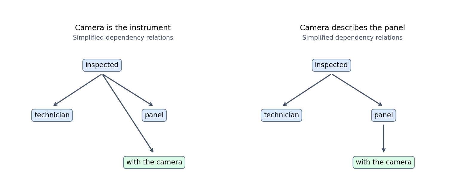
Under event attachment, a camera is the instrument of inspection. Under noun attachment, the camera helps identify the panel. Surrounding context can favor either: a technician explaining a recording method versus someone distinguishing equipped and unequipped panels. Grammatical possibility does not determine which situation actually occurred.
This is a preview. NLP 12 develops grammars, chart parsing, probabilistic parsing and dependency parsing. Here the essential question is what a representation must preserve: grouping, linked heads, role direction and plausible alternatives.
6. Semantics: meanings and truth conditions
Plain version. Semantics asks what an expression means and what the world would have to be like for a sentence to be true. Word meanings matter, but so does how the sentence combines them.
A sentence can be fluent while describing a situation incorrectly. Semantics asks how expressions contribute meaning and how a structured sentence determines conditions under which its assertion is true [2, 3]. Separating these conditions from conversational inference makes ambiguity easier to analyze.
Lexical meaning is contextual and relational
Polysemy concerns related senses of an expression; homonymy concerns distinct meanings sharing a form [3]. A window can be an opening in a wall or a bounded area on a screen. The relationship helps explain the extension, but replacing “window” with one fixed concrete object would miss the screen reading. A dictionary can list senses; the occurrence still needs interpretation. NLP 04 studies how vectors learned from contexts capture some of these relations.
Chinese 開 appears in 開門 (“open a door”) and 開會 (“hold a meeting”). Translating every occurrence with the same English verb would erase the construction-specific difference. Meaning belongs to the expression in its combination and context, not to a context-free lookup from character to English word.
Even apparently simple adjectives can rely on a comparison class. A small elephant may be larger than a large ant. The expressions compare each animal with an appropriate class, not with one universal size threshold. In a collection containing only toy elephants, the relevant comparison can change again. An annotation called “small” should therefore specify what is being compared.
Composition depends on structure
Compositionality is the idea that the meaning of a complex expression depends on meanings of its parts and how they combine [3]. It does not say that word meanings can simply be added together. “Bo praised Ada” combines participants in a directed relation; a reordered sentence combines the same names differently. Attachment changes which expression a modifier restricts.
An idiomatic expression can also have a conventional meaning not predictable from isolated word entries. A lexicon and a grammar are complementary: the analysis must record both conventional combinations and productive composition. For an application, ask which distinction is needed. Searching for repair instructions may tolerate broad lexical grouping; deciding whether a repair was completed requires event, tense and negation information.
Quantifier scope changes what is required
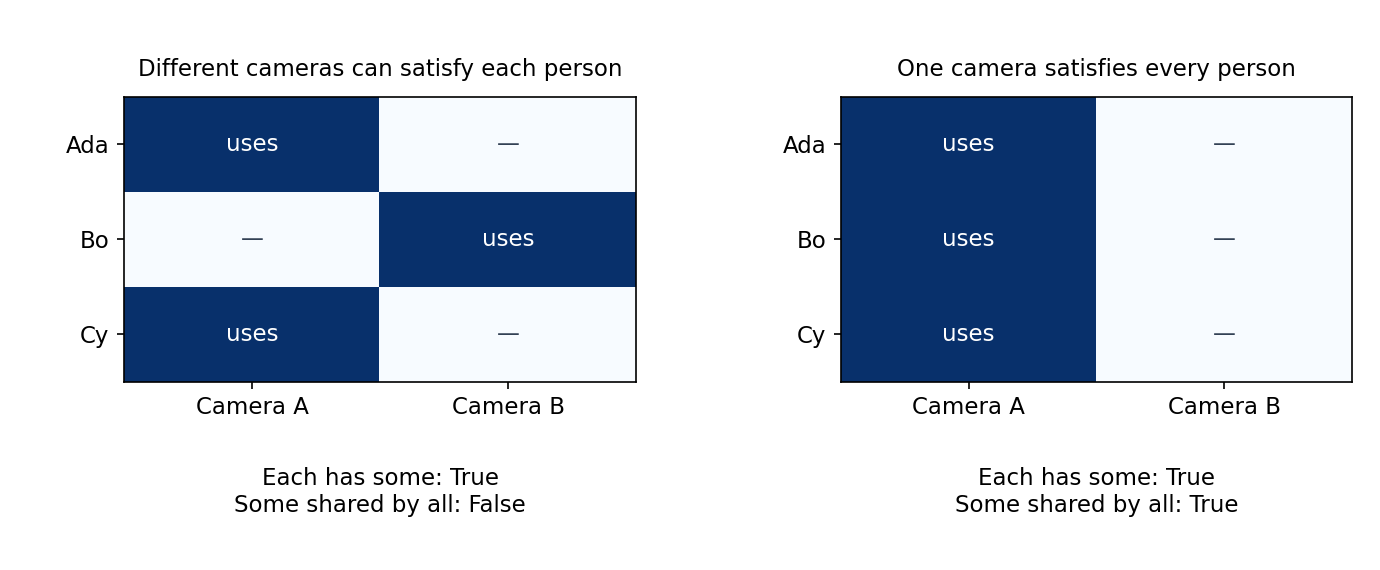
“Every technician uses a camera” has a reading in which different technicians may use different cameras. It can also be understood, in a suitable context, as involving one camera shared by all. These are different conditions:
Here is the set of technicians, the set of cameras, means technician uses camera , and name the two readings, means “for every,” and means “there exists.” Both sets are nonempty in this example. The variable can depend on in ; in one must work for every .
To check , visit each technician and find at least one camera they use. To check , choose a camera first and verify that all technicians use that particular camera. If holds, follows: use the shared camera for each person. The reverse implication fails when every person has a camera but no camera is shared by everyone.
Code · Python · 14 lines
technicians = ("Ada", "Bo", "Cy")
cameras = ("A", "B")
worlds = {
    "distributed": {("Ada", "A"), ("Bo", "B"), ("Cy", "A")},
    "shared": {("Ada", "A"), ("Bo", "A"), ("Cy", "A")},
}
for name, uses in worlds.items():
    each_has_some = all(any((t, c) in uses for c in cameras)
                        for t in technicians)
    some_for_everyone = any(all((t, c) in uses for t in technicians)
                           for c in cameras)
    print(name, each_has_some, some_for_everyone)
assert not any(all((t, c) in worlds["distributed"] for t in technicians)
               for c in cameras)
The outputs are distributed True False and shared True True. Each row in Figure 3 represents one person’s possibilities. The first reading requires a marked cell in every row; the second requires an entirely marked column. Scope is therefore a constraint difference, not merely a different paraphrase of the same requirement.
Negation and scope must also be kept apart
“Not every technician approved” allows some approvals and at least one non-approval. “Every technician did not approve,” under a reading with negation inside the universal quantifier, says that nobody approved. Written English can itself leave scope unclear; explicit paraphrases remove the ambiguity.
The Chinese contrast 不是每位技師都批准 / 每位技師都不批准 makes the intended distinction easier to display. The former negates “all approved”; the latter assigns non-approval to each technician. For a nonempty technician set:
Here is the technician set, means approved, is negation, and are universal and existential quantification, and means logical equivalence. The first condition needs one counterexample to universal approval; the second excludes every approval. If one technician approves and another does not, only the first condition is true.
NLP 12 develops predicate–argument structure and semantic role labeling, and NLP 11 tests inference between sentences. Before designing a field such as approved, decide whose approval, what event and which quantified claim that field represents.
7. Pragmatics: interpretation in a situation
Plain version. What a speaker means can go beyond what the sentence literally says. Pragmatics studies how the situation fills that gap.
Speakers often communicate more than their sentence literally asserts. Pragmatics studies language use in context, including reference, background assumptions and communicative actions [9, 10]. Context supplies evidence; it does not license arbitrary interpretations.
Reference and the speaker’s viewpoint
“I will check that here tomorrow” is structurally simple but under-specified outside its setting. “I” identifies the speaker, “that” selects a referent, “here” uses a spatial viewpoint, and “tomorrow” uses a temporal viewpoint. Such context-dependent expressions involve deixis [10]. A forwarded message should not silently replace the original speaker’s time and place with the receiver’s.
Reference also depends on discourse. “Mei put a camera beside a lamp. It was overheating.” Either object may be the referent of “it” without further evidence. Knowing that cameras and lamps can both become hot leaves the ambiguity intact. In “Mei turned off the lamp. It stopped flickering,” the described event supplies evidence favoring the lamp. Evidence may favor a candidate without turning a grammatical possibility into a universal rule.
A practical analysis records the expression, candidate referents and supporting context. An unresolved referent is a meaningful result when the input does not determine one. Coreference resolution across sentences is developed in NLP 12, and tracking entities across dialogue turns in NLP 08.
Assertion, presupposition and implicature
An assertion contributes the claim at issue. A presupposition presents a proposition as background rather than as the main update. A conversational implicature is an additional inference drawn from the utterance and its use, which can often be cancelled without contradicting the literal assertion [9, 10]. They should not collapse into one “meaning” label.
“Mei stopped checking the sensor” asserts a cessation and normally backgrounds that Mei checked it previously. “Mei did not stop checking the sensor” still typically takes earlier checking for granted. That persistence under negation helps diagnose the background contribution. These are ordinary interpretations, not a proof that the earlier event actually occurred. A listener can challenge it: “She never checked it in the first place.”
“Some panels passed” asserts that at least one panel passed in the relevant collection. In a conversation asking whether the whole collection passed, a listener may infer “not all.” But “Some panels passed; in fact, all of them did” can cancel that inference without denying the first assertion [9]. By contrast, “All panels passed; in fact, one failed” conflicts under the same panel collection, test and time.
This difference can be checked without a language model. Imagine three panels: one, two and three passing panels all satisfy the literal “some.” A “some but not all” interpretation retains only the first two possibilities. The inference narrows the possibilities because of a conversational expectation; that narrowing is not contributed by existential meaning alone. Whether it is justified depends on the question, speaker knowledge and manner of reporting.
A grammatical question can perform a request
“Can you lower the gain?” has the form of an ability question. During a recording session, it can perform a request to change a setting; during an assessment, it can ask whether the trainee knows how [10]. A speech act is the communicative action performed through an utterance, such as requesting, promising, asserting or asking.
“The gain is too high” can likewise function as a report or an indirect request. The physical words do not themselves specify every interpersonal condition. Who controls the equipment? What was the preceding question? Is the speaker diagnosing the recording or coordinating an adjustment? These details support an interpretation of the action.
A useful annotation separates sentence form, asserted content and intended act. Otherwise, every question-shaped request may be labeled as information seeking, or every unfavorable description may be labeled as an instruction. The goal is a defensible reading of this interaction, including alternatives when the setting is missing.
8. Discourse: meaning across sentences and turns
Plain version. Sentences in a text or a conversation lean on each other. Later sentences refer back, contrast, explain or correct, and a reader keeps track of that shared state.
An utterance can introduce an entity, correct an earlier claim, provide a reason or contrast with an expectation. Discourse analysis considers these connections across sentences and conversational turns [2, 10]. Reading each sentence independently discards the shared state that makes later expressions interpretable.
“Mei told Lin that she would calibrate the camera” can refer to either person as the future calibrator. The Chinese 美玲告訴怡君,她會校正相機 permits a comparable ambiguity in this invented setting. A preceding statement “Lin had already volunteered” favors Lin; “Mei was the only available technician” favors Mei. Neither grammatical gender nor mention order alone settles both contexts.
Now compare “The sensor became hot. Its readings stayed stable” with “The sensor became hot, but its readings stayed stable.” The second explicitly marks a contrast with an expectation that heat would disrupt readings. The assertion about stability can be the same while the discourse contribution differs. Conversely, “The readings drifted because the sensor became hot” introduces a causal explanation, not merely two events in sequence.
Conversations also contain repairs. “Move it to Friday.” “The inspection?” “Yes, the inspection.” The middle turn does not advance the scheduling date; it resolves the object. Once resolved, later references can use the shared identification. A dialogue system that summarizes only the first and last words misses why the clarification changed the conversational state.
This suggests a practical representation with distinct records for introduced entities, asserted events, unresolved references and conversational questions. Such a representation can remain partial. A one-sentence input may leave the speaker unknown; an entire exchange may resolve the speaker but still leave the exact camera unspecified. Increasing context length only helps when relevant evidence is actually present.
9. Corpora, annotation and Zipf’s law
Plain version. NLP learns from collections of real text, often with human labels added. How the text was collected and how consistently it was labeled limit what any model can learn from it, and every corpus has a long tail of rare words.
A corpus is a collection of text or transcribed speech gathered under stated decisions: which sources, which period, which speakers, which language varieties. An annotated corpus adds analyses such as segmentation, tags, trees, entity spans or sentiment labels, produced under written guidelines. Two widely used examples show the range. The Penn Treebank annotated English text with part-of-speech tags and constituency trees [26]. The Universal Dependencies project releases treebanks for many languages under one cross-lingual dependency scheme [24]. The segmentation bakeoff corpora above show that even word boundaries come with a standard attached [27].
Annotation guidelines and agreement
A label is only as clear as the guideline behind it. Two careful annotators can disagree because a sentence is genuinely ambiguous, because the guideline is silent, or because one of them made an error. Measuring agreement on a shared sample separates these cases before the labels are used for training.
Raw percent agreement overstates reliability when one label is very common, because annotators would agree often even by guessing. Cohen’s kappa corrects for that [28]:
Here is the observed fraction of items on which annotators and agree; is the agreement expected if each annotator chose labels independently at their own observed rates; is the label set; and count how often each annotator used label ; and is the number of items. is perfect agreement and is agreement at the chance level; the formula requires .
Code · Python · 14 lines
from collections import Counter
from sklearn.metrics import cohen_kappa_score

words = "Mei has to repair the camera mount before the inspection".split()
a = "PROPN VERB PART VERB DET NOUN NOUN ADP DET NOUN".split()   # annotator A
b = "PROPN AUX ADP VERB DET NOUN NOUN ADP DET NOUN".split()     # annotator B
n = len(words)
p_o = sum(x == y for x, y in zip(a, b)) / n                     # observed agreement
ca, cb = Counter(a), Counter(b)
p_e = sum(ca[k] * cb[k] for k in ca) / n**2                     # agreement expected by chance
kappa = (p_o - p_e) / (1 - p_e)
print(f"p_o={p_o:.3f}  p_e={p_e:.3f}  kappa={kappa:.3f}")
assert abs(kappa - cohen_kappa_score(a, b)) < 1e-12
print("disagreements:", [(w, x, y) for w, x, y in zip(words, a, b) if x != y])
It prints p_o=0.800 p_e=0.180 kappa=0.756, and the two disagreements are has (VERB versus AUX) and to (PART versus ADP). Neither is a careless slip: “has to” sits on the border between a main verb and an auxiliary, and infinitival “to” resembles a preposition. The useful outcome is a guideline decision for that construction, not a higher number. Kappa summarizes reliability; the disagreement list says what to fix.
Zipf’s law: a few words are very common, most are rare
Count every word in a corpus and sort the types by frequency. A handful of function words such as “the” and “of” account for a large share of all tokens, while a huge number of types occur only once or twice. Zipf’s law describes the relation between a word’s frequency rank and its count as approximately a power law [29]:
Here is a type’s rank when types are sorted by decreasing count, is the count of the type at rank , is a scale constant and is the exponent. With , the product stays roughly constant. On log–log axes the relation is a straight line with slope . Piantadosi’s review shows that the law holds approximately across many languages and corpora, that it deviates systematically at the extremes, and that its explanation is still debated [29].
We can check it on real English text that is already on disk: the docstrings of the Python standard library installed in the project environment (Python 3.9).
Code · Python · 22 lines
import ast, re, sysconfig
from collections import Counter
from pathlib import Path

lib = Path(sysconfig.get_paths()["stdlib"])        # text already on disk: stdlib docstrings
docs = []
for path in sorted(lib.glob("*.py")):
    try:
        tree = ast.parse(path.read_text(encoding="utf-8"))
    except (SyntaxError, UnicodeDecodeError):
        continue
    docs += [ast.get_docstring(n) or "" for n in ast.walk(tree)
             if isinstance(n, (ast.Module, ast.FunctionDef, ast.AsyncFunctionDef, ast.ClassDef))]
tokens = [w for d in docs for w in re.findall(r"[a-z]+", d.lower())]
counts = Counter(tokens)
print(len(tokens), "tokens,", len(counts), "types")
ranked = counts.most_common()
for r in (1, 2, 10, 100, 1000):
    word, f = ranked[r - 1]
    print(f"rank {r:4d}  {word:10s} f={f:5d}  r*f={r * f}")
hapax = sum(f == 1 for f in counts.values())
print(f"types seen once: {hapax} ({hapax / len(counts):.0%})")
With Python 3.9.7 it finds 134,620 tokens and 6,281 types. The product is 8,313 at rank 1 (“the”), 13,640 at rank 10 (“be”), 20,100 at rank 100 (“called”) and 18,000 at rank 1,000: not constant, but within a factor of about 2.5 while the rank changes by a factor of 1,000. A least-squares fit over ranks 10 to 1,000 in the figure script gives . A third of all types, 2,003 of them (32%), occur exactly once. A different Python version ships different docstrings, so the exact counts can change.
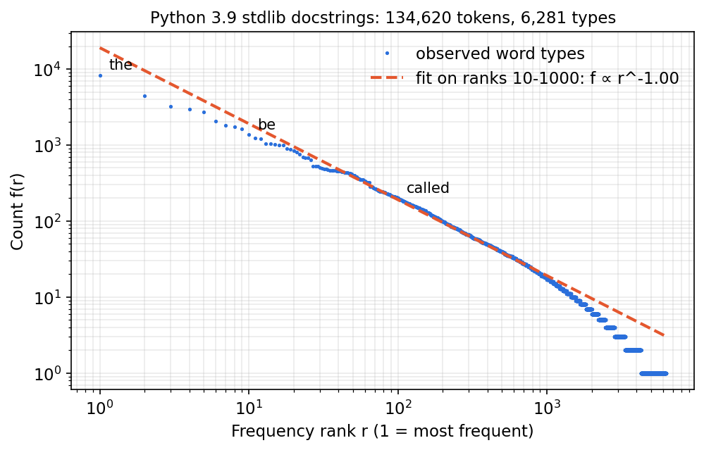
Three consequences follow for NLP. First, any fixed word vocabulary leaves out part of the tail, so new text keeps producing unseen words; this is why subword vocabularies exist. Second, count-based probability estimates are reliable for frequent words and unreliable for the rare majority, which is why smoothing appears in n-gram models (NLP 05). Third, accuracy on all tokens is dominated by frequent words; an evaluation that matters for rare names or technical terms must measure them separately.
10. Linguistic diversity and model assumptions
Plain version. Languages package information differently, and communities speak and write in different varieties. A model built around one language’s habits can miss what another language says.
Languages and communities distribute information differently across morphology, order, prosody and context. Typology compares such structural patterns. Dialect concerns a community’s variety; register concerns usage associated with a setting or activity [3, 11]. These distinctions describe variation rather than rank ways of speaking.
Translation does not preserve every structure
Compare “I calibrated this camera yesterday” with 這台相機,我昨天校正過. The Chinese example begins with the camera as the topic and then comments on it. Treating the first noun phrase as the actor would misidentify the calibrator. An English translation can preserve the event while changing how the message organizes old and new information.
The short Chinese 已經校正好了 can be informative when the camera and responsible person are already established. A word-for-word translation that demands overt counterparts for every English argument may make it look incomplete. In context it can answer a pending question directly. This does not mean that any omitted participant is always recoverable; the analysis must examine the actual discourse.
Similarly, 三台相機 and “three cameras” package number differently. A feature called “plural suffix” cannot be required universally merely because it suits one language. Structural categories may be useful for comparison while needing language-specific realizations and annotation decisions. A language using fewer obligatory endings can still express detailed distinctions through constructions, words and context.
Variety, setting and mixed-language expression
A formal maintenance report and a chat between technicians can describe the same equipment with different vocabulary, abbreviation and explicitness. The report “The shutter failed to actuate” and the informal “The shutter didn’t fire” may describe a related event in context, yet the wording provides different evidence about setting and intended readership. Unfamiliar wording is not automatically an error.
A speaker might write 把 exposure 調低一點 in a bilingual discussion. The English item occupies a position in an otherwise Chinese construction. Code-switching involves alternation between linguistic varieties within an interaction [14]; analyzing this example requires both the lexical choice and the surrounding grammar. One occurrence alone may not settle whether a community treats the item as switching or as an established borrowing.
An analysis should preserve the observed expression before standardizing it. Replacing a regional or technical expression with a presumed standard can help a particular search task, but may erase a distinction needed for another task. A corpus records language from particular speakers, settings and collection decisions; frequent corpus patterns are evidence of usage, not a universal inventory of everything speakers can say.
11. A complete worked reading
Put the levels together with an invented message:
小林說:「那台相機又過熱了,你明天能幫我看看嗎?」
Lin said: “That camera overheated again. Can you take a look for me tomorrow?”
The translation helps an English reader but already chooses wording for 看看 and punctuation for the quoted interaction. Analyze the original before treating the translation as equivalent evidence.
| Level | What the message contributes | What remains to be established |
|---|---|---|
| Written form and segmentation | The quotation groups Lin’s utterance; 相機 is a camera expression | Speech intonation and gesture are absent |
| Morphology and construction | 看看 is a reduplicated form in this request, not a counted pair of inspections | Exact activity and expected effort depend on the setting |
| Syntax | 小林 introduces the reported speaker; 你 is the addressee inside the quotation | The reporter need not be the addressee |
| Semantics | The camera is described as overheating; a future assistance question is expressed | Which camera, and whether the description is factually correct |
| Background and reference | 又 normally invokes a prior occurrence; 那台 selects a contextually identified camera | Prior overheating and the demonstrative referent require evidence |
| Pragmatics and discourse | The question naturally supports a request in a maintenance conversation | Whether that reading fits this interaction and whether it is accepted |
The quotation changes the reference frame. “我” refers to Lin as the quoted speaker. “你” refers to Lin’s addressee, who may differ from the current reader. “明天” is relative to the quoted utterance’s day. If the report arrives later, its arrival date does not redefine the requested day.
The ordinary reading of 看看 presents the activity as taking a look, often with a light or tentative framing in this construction [13]. It does not establish a precise inspection duration or a numerical repetition count. Translating it as “inspect twice” would confuse visible repetition with event counting.
Finally, separate linguistic evidence from factual evidence. The message provides evidence that Lin reported overheating and requested help. It does not by itself verify overheating, identify a serial number or show that anyone agreed to help. A structured output might record the speaker and reported event while retaining unresolved referents and dates. This is a more informative analysis than assigning a single topic label such as “camera repair.”
Modern view
Recent surveys show why language analysis remains necessary for large language models. Ma and colleagues’ 2025 survey organizes pragmatic evaluation by phenomena including reference and deixis, implicature and presupposition, speech acts, discourse and social pragmatics [10]. It compares task design, collection and evaluation, and identifies gaps between available tests and contextual language use. Its useful lesson here is to evaluate the particular inference required, rather than treating a broad language score as proof of all pragmatic abilities.
Mielke and colleagues’ tokenization review organizes the open-vocabulary problem across words, characters and intermediate units [22]. Its useful question is how segmentation balances coverage, sequence length and reuse. These quantities remain distinct: a tokenizer can represent every input string while giving a model little training evidence for the relevant combinations. Zipf’s law explains why the problem never goes away: however large the vocabulary, the tail keeps supplying rare forms [29].
Qin and colleagues’ 2025 survey separates multilingual alignment through parameter tuning from alignment with frozen parameters, including prompting and translation-based approaches [12]. It reviews cross-language training, evaluation and challenges. This distinction identifies where a system’s behavior is being adapted, but multilingual output alone does not establish that it preserves a construction’s scope, register or conversational force.
Winata and colleagues’ 2023 systematic survey groups code-switching research by languages, tasks and research trends [15]. Read it alongside Doğruöz and colleagues’ account of structural and social patterns [14]: testing on text assembled from two monolingual sources is a different task from interpreting how bilingual speakers actually switch during an interaction. The exposure example in Section 10 makes that distinction concrete: the surrounding construction and conversational setting contribute information beyond identifying the English item.
Linguistic analysis also continues to refine apparently simple constructions. Lu and Müller’s 2026 study analyzes Mandarin verb reduplication and its interaction with verb classes and aspect [13]. For this tutorial, the relevant observation is that limited-event meaning and context-dependent pragmatic effects deserve separate analysis. Visible repetition is not a general instruction to count events twice.
A concrete evaluation can vary one property while holding others fixed. Reverse Ada and Bo to test role direction; change camera attachment while preserving words; compare “not all” with “none”; move a quoted message into a later reporting context. Write the expected interpretations and acceptable alternatives first. Then a failure reveals which distinction was lost. These examples are small diagnostic tests, not a claim that passing them establishes general language competence.
Open problems include recovering relevant context, distinguishing genuine ambiguity from avoidable annotation disagreement, evaluating naturally mixed-language conversation and measuring interpretation across communities rather than only translated prompts. Some inputs legitimately admit several readings. A system that states the alternatives and the missing evidence may be more faithful to the language than one that confidently chooses a single answer.
Key takeaways
- Spoken, signed and written language expose different information; a transcript is a partial record.
- Computational tokens need not coincide with words, morphemes, lexemes or sound units; subword pieces from BPE, WordPiece or a unigram model reflect frequency, not morphology.
- Stemming strips endings by rule; lemmatization maps to a dictionary form and needs the part of speech. Both discard information some tasks need.
- Morphological structure and Chinese segmentation encode analytical choices with possible alternatives, and corpora follow different standards.
- Word counts discard order; part-of-speech categories, grouping and grammatical relations carry additional meaning. Constituency shows groups, dependency shows heads.
- Scope determines truth conditions: “each has some” need not mean “some shared by all.”
- Assertion, background assumptions, cancellable inferences, reference, speech acts and discourse relations require the speaker’s situation and conversational history.
- Corpora come with collection choices and annotation guidelines; check agreement, and expect a Zipfian long tail of rare words.
Exercises
- For “The technician repaired two cameras,” identify a word form, a lexeme, an inflectional contrast, a UPOS tag sequence and a possible computational tokenization. Explain what each representation preserves.
Hint
Compare “repaired” with REPAIR. A tokenizer could keep the whole form or split it; neither choice alone establishes the tense interpretation, which UD records as a feature.
- Add one sentence of context for each reading of 學生會說話. Explain why the lexicon enumeration alone cannot prefer either context.
Hint
One setting can concern students’ abilities; another can concern a student council announcing its position.
- Change one training word’s frequency in the BPE corpus. Inspect the first merge and encode
lowestagain. Why need neither result remain unchanged?
Hint
Pair counts are weighted by word occurrence counts. An early merge changes the pairs available later.
- Write two contexts for “The technician inspected the panel with the camera,” one for each attachment. Identify which head receives the modifier and how the event description changes.
Hint
Contrast the inspection method with identifying a camera-equipped panel among several panels.
- Modify the quantifier program to add a technician who uses no camera. Predict both readings before running it, then explain the implication from to .
Hint
Both conditions fail if any technician has no usable pair. A single shared camera supplies a witness for every technician.
- Analyze “Mei stopped checking the sensor” and “Some panels passed” separately under negation and explicit cancellation. Distinguish the main assertion, ordinary background assumption and conversational inference.
Hint
Try “Mei never checked it” as a challenge to background and “in fact, all passed” as cancellation of an inference. Keep the panel collection and test fixed.
References
- Masato Hagiwara, Real-World Natural Language Processing: Practical Applications with Deep Learning, Manning, 2021. Publisher
- Susan McRoy, Principles of Natural Language Processing, University of Wisconsin–Milwaukee open textbook, 2021. Grammars and Syntactic Processing
- Catherine Anderson, Bronwyn Bjorkman, Derek Denis, Julianne Doner, Margaret Grant, Nathan Sanders and Ai Taniguchi, Essentials of Linguistics, 2nd ed., eCampusOntario, 2022. Open textbook
- Catherine Anderson et al., “3.1 Modality,” Essentials of Linguistics, 2nd ed., eCampusOntario, 2022. Chapter
- Catherine Anderson et al., “4.1 Phonemes and allophones,” Essentials of Linguistics, 2nd ed., eCampusOntario, 2022. Chapter
- Catherine Anderson et al., “3.12 Tone and intonation,” Essentials of Linguistics, 2nd ed., eCampusOntario, 2022. Chapter
- Catherine Anderson et al., “5.1 What is morphology?,” Essentials of Linguistics, 2nd ed., eCampusOntario, 2022. Chapter
- Catherine Anderson et al., “6.4 Identifying phrases: Constituency tests,” Essentials of Linguistics, 2nd ed., eCampusOntario, 2022. Chapter
- Catherine Anderson et al., “8.4 Conversational implicatures,” Essentials of Linguistics, 2nd ed., eCampusOntario, 2022. Chapter
- Bolei Ma, Yuting Li, Wei Zhou, Ziwei Gong, Yang Janet Liu, Katja Jasinskaja, Annemarie Friedrich, Julia Hirschberg, Frauke Kreuter and Barbara Plank, “Pragmatics in the Era of Large Language Models: A Survey on Datasets, Evaluation, Opportunities and Challenges,” ACL, pp. 8679–8696, 2025. Paper
- Catherine Anderson et al., “10.2 Language varies,” Essentials of Linguistics, 2nd ed., eCampusOntario, 2022. Chapter
- Libo Qin, Qiguang Chen, Yuhang Zhou, Zhi Chen, Yinghui Li, Lizi Liao, Min Li, Wanxiang Che and Philip S. Yu, “A survey of multilingual large language models,” Patterns, 6(1), 101118, 2025. Paper
- Yanru Lu and Stefan Müller, “Deliminative verbal reduplication in Mandarin Chinese,” Journal of Linguistics, 62(3), pp. 595–632, 2026. Paper
- A. Seza Doğruöz, Sunayana Sitaram, Barbara E. Bullock and Almeida Jacqueline Toribio, “A Survey of Code-switching: Linguistic and Social Perspectives for Language Technologies,” ACL-IJCNLP, pp. 1654–1666, 2021. Paper
- Genta Winata, Alham Fikri Aji, Zheng Xin Yong and Thamar Solorio, “The Decades Progress on Code-Switching Research in NLP: A Systematic Survey on Trends and Challenges,” Findings of ACL, pp. 2936–2978, 2023. Paper
- M. F. Porter, “An algorithm for suffix stripping,” Program, 14(3), pp. 130–137, 1980. DOI
- Rico Sennrich, Barry Haddow and Alexandra Birch, “Neural Machine Translation of Rare Words with Subword Units,” ACL, 2016. Paper
- Mike Schuster and Kaisuke Nakajima, “Japanese and Korean Voice Search,” ICASSP, pp. 5149–5152, 2012. DOI
- Yonghui Wu et al., “Google’s Neural Machine Translation System: Bridging the Gap between Human and Machine Translation,” arXiv:1609.08144, 2016. Paper
- Taku Kudo, “Subword Regularization: Improving Neural Network Translation Models with Multiple Subword Candidates,” ACL, 2018. Paper
- Taku Kudo and John Richardson, “SentencePiece: A Simple and Language Independent Subword Tokenizer and Detokenizer for Neural Text Processing,” EMNLP System Demonstrations, 2018. Paper
- Sabrina J. Mielke et al., “Between Words and Characters: A Brief History of Open-Vocabulary Modeling and Tokenization in NLP,” arXiv:2112.10508, 2021. Review
- Hugging Face, “The Tokenization Pipeline,” Tokenizers documentation, current online edition. Documentation
- Marie-Catherine de Marneffe, Christopher D. Manning, Joakim Nivre and Daniel Zeman, “Universal Dependencies,” Computational Linguistics, 47(2), 2021. Paper
- Universal Dependencies contributors, “Universal POS tags,” Universal Dependencies documentation, current online edition. Documentation
- Mitchell P. Marcus, Beatrice Santorini and Mary Ann Marcinkiewicz, “Building a Large Annotated Corpus of English: The Penn Treebank,” Computational Linguistics, 19(2), 1993. Paper
- Thomas Emerson, “The Second International Chinese Word Segmentation Bakeoff,” Proceedings of the Fourth SIGHAN Workshop on Chinese Language Processing, 2005. Paper
- Jacob Cohen, “A Coefficient of Agreement for Nominal Scales,” Educational and Psychological Measurement, 20(1), pp. 37–46, 1960. DOI
- Steven T. Piantadosi, “Zipf’s word frequency law in natural language: A critical review and future directions,” Psychonomic Bulletin & Review, 21(5), pp. 1112–1130, 2014. DOI
- Jacob Devlin, Ming-Wei Chang, Kenton Lee and Kristina Toutanova, “BERT: Pre-training of Deep Bidirectional Transformers for Language Understanding,” NAACL-HLT, 2019. Paper
Check your understanding
This tutorial has 6 exercises. Can you solve them without opening the hints?
Go to the exercises ↑Next NLP 03 · Neural Networks for NLP · 34 min