NLP 03 · Neural Networks for NLP
Needs: NLP 02 · Linguistic Essentials, ML 02 · Neural Networks from Perceptron to Deep Networks
Navigate: this page and this track: Navigate: this page and this track
On this page
- What you’ll learn1 min
- The big picture2 min
- Define the prediction contract1 min
- Count features and the vocabulary1 min
- TF–IDF and vector normalization1 min
- Logistic classification and its loss2 min
- A complete CPU classification experiment2 min
- A controlled negation test1 min
- From word IDs to learned vectors: the embedding layer2 min
- The neural probabilistic language model2 min
- Convolutional text classifiers4 min
- Padding, masking and batching2 min
- Regularization for small text classifiers1 min
- A complete PyTorch experiment3 min
- Evaluate errors and probabilities separately1 min
- Imbalance, error analysis and deployment changes2 min
- Modern view2 min
- Key takeaways1 min
- Exercises2 min
- Paper guides
- References
Natural Language Processing
Explore this chapter 2 interactive experiments
Compare a fixed two-unit network with and without nonlinear activations on the XOR corners.
What you’ll learn
- Define a text classification task with explicit annotation rules, then derive count features, TF–IDF, logistic classification and cross-entropy.
- Turn token IDs into learned vectors with an embedding layer, pool them, and classify with a small multilayer perceptron.
- Follow the neural probabilistic language model of Bengio et al. and explain why shared word vectors let it generalize to unseen histories.
- Write the mathematics of a 1-D convolutional text classifier with max-over-time pooling, and implement it with correct padding and masking.
- Regularize, train and early-stop a small PyTorch model, read its training curves and analyze its errors by category.
- Evaluate decisions, probability quality, coverage and class imbalance separately.
The big picture
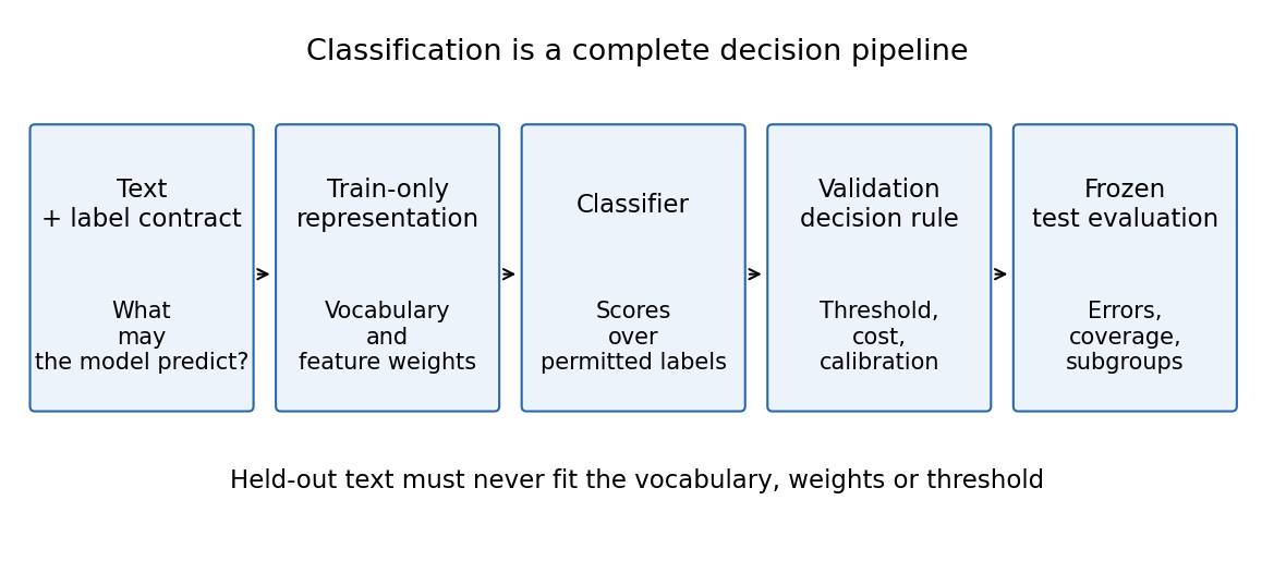
A text classifier converts a message into a permitted decision: route a complaint, identify a language, label a review or flag a document for inspection. Its most consequential choices often occur before the neural architecture is selected. What counts as one example? Which context is visible? What does the label mean? What should happen when none of the available labels fits?
Hagiwara develops a first classification application, word and document embeddings, sentence classification and convolutional encoders in Chapters 2–4 and 7 [1]. McRoy’s Chapter 6 distinguishes sentiment, similarity, grammaticality and entailment as different language tasks [2]. This lesson follows that combination: build an application, but make its prediction target precise. A sentiment label is not an entailment judgment, and a similarity score is not a statement that two claims have the same truth conditions.
The lesson has two halves. The first builds the strongest simple baseline: sparse features and a linear classifier, trained and evaluated with care. The second replaces hand-designed features with learned ones: an embedding layer, a pooled multilayer perceptron, the neural probabilistic language model and a convolutional encoder. Every neural model here is still trained with the same cross-entropy loss as the linear baseline, so the change is in the representation, not the objective. Backpropagation, activation functions and optimizers are developed in ML 02; this page uses them and focuses on what is specific to text.
All examples use invented messages and require no dataset download. Measured scores describe these synthetic messages; they cannot establish performance on an actual application.
Define the prediction contract
Plain version. A label is an agreement about what a piece of text means for this application. Establish that agreement before collecting examples or optimizing a loss.
In single-label classification, one input receives exactly one label from a fixed set. In multi-label classification, several labels may apply simultaneously. A complaint about both a delayed parcel and an incorrect charge may require two routes, a primary route with secondary tags, or a human triage decision. These are different tasks even if the input text is identical.
Write the contract in ordinary language first. For our toy application, billing concerns a payment or invoice, delivery concerns a parcel or shipping, and technical concerns account access or software behavior. We permit an abstention action after classification. An ambiguous multi-topic message is therefore not silently forced into a category merely because the numerical model has an argmax.
Here is a classifier with learned parameters , is the set of allowed text inputs, is the simplex of probability vectors over classes, is one input, is its label, indexes a class, is the model’s conditional distribution and is its most probable class. The simplex requires nonnegative entries whose sum is one.
This equation describes a model output, not the whole product action. The service may return a route only when confidence passes a validation-selected threshold. It may also reject an empty message, ask for additional context or send a multi-topic message to review. Those actions should be visible in evaluation.
Keep the unit of supervision aligned with deployment. A sentence-level sentiment model trained on isolated opinions may fail on a whole conversation containing quotations, corrections and several speakers. If deployment includes previous turns, annotation and training should include the same permitted context. Conversely, giving annotators access to the final resolution while the model only sees the first message creates an impossible target.
Count features and the vocabulary
Plain version. The simplest useful representation records which words or short sequences occur. It is inexpensive, inspectable and often an excellent first comparison.
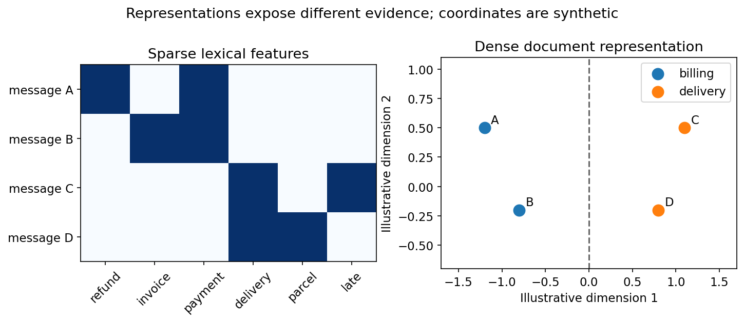
Choose a vocabulary from training text only. Its entries might be words, character sequences or consecutive word pairs. For a word vocabulary, each coordinate counts one vocabulary entry. A document becomes a sparse vector because most possible words are absent.
Here is a document, is the vocabulary item at coordinate , is its occurrence count in , is that feature value, is the resulting column vector and is the vocabulary size. The transpose symbol specifies that the listed coordinates form a column.
This bag-of-words representation ignores order. “Payment arrived after the refund” and “Refund arrived after the payment” contain the same words but describe different event orders. Word bigrams recover some local information, while character features can capture spelling fragments and inflections. Neither automatically understands a long dependency or the scope of a negation.
Feature choices encode useful assumptions. Lowercasing can reduce sparsity, but it merges names with common nouns. Removing every stop word can remove “not,” which is essential to many classifications. A language detector may benefit from character patterns rather than a word vocabulary tailored to one language. Use the task definition to justify each normalization rule; NLP 02 discusses the linguistic units behind these choices.
Fit vocabulary construction, document-frequency thresholds and any feature selection inside the training portion of each experiment. Looking at test documents to decide which rare terms to retain gives the training pipeline information about the evaluation distribution. It can be subtle leakage even when no test label is read.
Keep a record of vocabulary size, proportion of messages with no recognized features, token counts and representative discarded terms. These diagnostics reveal changes that a single accuracy score hides. A new product code or language can make many inputs nearly empty without causing an obvious exception.
TF–IDF and vector normalization
Plain version. A word that occurs in almost every message is usually less useful for distinguishing messages. TF–IDF balances occurrence within a document against rarity across training documents.
One common smoothed definition, used by the implementation here, is:
Here is the inverse-document-frequency weight for vocabulary entry , is the number of training documents, counts training documents containing that entry, is its count in document , is the weighted coordinate, collects those coordinates and is its unit-length version. The Euclidean norm is the square root of the sum of squared coordinates. A zero vector remains zero rather than being divided by zero. The scikit-learn feature-extraction documentation specifies these implementation choices [3].
The added ones prevent undefined weights for the fitted vocabulary and fix the precise smoothing convention. Other libraries use other conventions, so “TF–IDF” alone is not a complete reproducibility statement. Record the tokenizer, feature range, count transformation, weighting formula and normalization.
Normalization makes a long message less dominant simply because it repeats words. That helps when direction in feature space matters more than total length. But length can itself be predictive: an error report might be longer than a password-reset request. If length is relevant, add an explicit length feature instead of relying on an accidental effect of unnormalized counts.
TF–IDF does not infer synonymy. “Charge” and “payment” remain different coordinates unless examples teach the classifier their similar role. It also weights rare identifiers strongly even when their rarity is irrelevant. An account number might look discriminative because a template is duplicated across related records. Grouped splitting and inspecting coefficients help reveal that shortcut.
Logistic classification and its loss
Plain version. A linear classifier adds evidence from features to produce one score per label. Turning scores into probabilities gives a differentiable training objective and a basis for decisions.
For a multiclass model:
Here is the score for class , is its learned feature-weight vector, is the normalized document representation, is a learned bias, is the conditional class probability, collects all weights and biases, is the document, indexes competing classes and is their number. The function is the exponential function.
The probability of the annotated class should increase during training. Regularization discourages arbitrarily large weights that fit incidental words:
Here is the objective, is the training-example count, indexes examples, is an annotated document and label, is the regularization strength, and is the sum of squared feature weights for class . The first term is multiclass cross-entropy; the second is squared-weight regularization. Library objectives can scale the terms differently; scikit-learn exposes inverse regularization through its parameter [4]. IT 01 explains why the first term is a cross-entropy.
A large positive coefficient says that a feature increases a class score relative to the other evidence. It does not prove that the feature causes the true category. Correlated words can share or exchange weight, and changing the vocabulary changes the meaning of a coefficient comparison.
For binary classification, the softmax can be written with one sigmoid of a score difference. For independent multi-label prediction, use a separate sigmoid per label rather than a softmax that forces labels to compete. Choose a loss and output activation that match the annotation contract, not whichever head happens to be easiest to implement.
Read as a network, this model is a single linear layer followed by a softmax. Every neural classifier below keeps that final layer and its loss. What changes is the vector : instead of being computed by a fixed counting rule, it is computed by learned layers.
A complete CPU classification experiment
Plain version. The vocabulary, classifier and threshold must learn from the intended portions of data. A pipeline makes this boundary easier to preserve.
The following standalone example uses invented messages. Training, validation and test text are explicitly separate. Validation selects a threshold using a stated illustrative cost: one wrong route costs two units, while asking for review costs one fifth of a unit. These values are policy parameters for this demonstration, not measured business costs. All choices freeze before the final test is inspected.
Code · Python · 85 lines
import numpy as np
from sklearn.pipeline import Pipeline
from sklearn.feature_extraction.text import TfidfVectorizer
from sklearn.linear_model import LogisticRegression
from sklearn.metrics import f1_score, log_loss

train = [
    ("please refund my payment", "billing"),
    ("the invoice has a wrong charge", "billing"),
    ("my payment was charged twice", "billing"),
    ("how can i update the billing card", "billing"),
    ("please send the payment receipt", "billing"),
    ("the refund is missing from my invoice", "billing"),
    ("where is my delivery parcel", "delivery"),
    ("my shipment is late", "delivery"),
    ("please change the delivery address", "delivery"),
    ("the parcel arrived damaged", "delivery"),
    ("how do i track the shipment", "delivery"),
    ("the delivery driver could not find the address", "delivery"),
    ("i cannot login to my account", "technical"),
    ("the application crashes on startup", "technical"),
    ("please reset my account password", "technical"),
    ("the software shows an error", "technical"),
    ("my login fails after the software update", "technical"),
    ("the application cannot connect to my account", "technical"),
]
validation = [
    ("i need a receipt for the charge", "billing"),
    ("the billing payment needs a refund", "billing"),
    ("can i track this delivery", "delivery"),
    ("the shipment went to another address", "delivery"),
    ("my password does not allow login", "technical"),
    ("the software crashes with an error", "technical"),
]
test = [
    ("please explain the invoice payment", "billing"),
    ("a charge appears before the refund", "billing"),
    ("the parcel delivery is not here", "delivery"),
    ("my shipment arrived at the wrong address", "delivery"),
    ("an account error prevents login", "technical"),
    ("the application crashes after a password change", "technical"),
]

def unpack(rows):
    return [text for text, _ in rows], np.array([label for _, label in rows])

train_x, train_y = unpack(train)
val_x, val_y = unpack(validation)
test_x, test_y = unpack(test)
model = Pipeline([
    ("features", TfidfVectorizer(ngram_range=(1, 2))),
    ("classifier", LogisticRegression(C=4.0, max_iter=300, random_state=0)),
])
model.fit(train_x, train_y)
classes = model.named_steps["classifier"].classes_

def decision(probabilities, threshold):
    best = probabilities.argmax(axis=1)
    prediction = classes[best]
    accepted = probabilities[np.arange(len(best)), best] >= threshold
    return prediction, accepted

val_prob = model.predict_proba(val_x)
grid = [0.40, 0.50, 0.60, 0.70, 0.80]
costs = []
for threshold in grid:
    pred, accepted = decision(val_prob, threshold)
    wrong = accepted & (pred != val_y)
    costs.append((2.0 * wrong.sum() + 0.2 * (~accepted).sum()) / len(val_y))
threshold = grid[int(np.argmin(costs))]  # first minimum fixes the tie rule

test_prob = model.predict_proba(test_x)
test_pred, accepted = decision(test_prob, threshold)
print("validation-selected threshold:", threshold)
print("test macro F1:", round(f1_score(test_y, test_pred, average="macro"), 3))
print("test log loss:", round(log_loss(test_y, test_prob, labels=classes), 3))
print("test coverage:", round(accepted.mean(), 3))
if accepted.any():
    print("accepted accuracy:", round((test_pred[accepted] == test_y[accepted]).mean(), 3))
else:
    print("accepted accuracy: undefined (no accepted messages)")
probe = ["the weather is pleasant", "my delivery charge is wrong"]
for text, probabilities in zip(probe, model.predict_proba(probe)):
    prediction, keep = decision(probabilities[None, :], threshold)
    print(text, "->", prediction[0] if keep[0] else "review")
The run prints:
Code · 7 lines
validation-selected threshold: 0.4
test macro F1: 1.0
test log loss: 0.413
test coverage: 1.0
accepted accuracy: 1.0
the weather is pleasant -> delivery
my delivery charge is wrong -> delivery
Six perfectly classified test messages are far too few to support any claim about the method; they only show that the pipeline runs end to end. The validation set made every threshold above 0.40 look costly, so the lowest grid value won, and the policy accepts everything.
The unfamiliar weather message is the useful part. None of the three routes is correct, yet the model still returns a probability distribution, and here its largest probability (about 0.51 for delivery) passes the selected threshold. The output head has no additional class for arbitrary outside topics. An abstention threshold can reduce some inappropriate actions, but a probability maximum is not a guaranteed out-of-domain detector, and in this run it does not catch the message at all. The mixed-topic “delivery charge” message is likewise forced into one route.
Notice that the final macro F1 measures forced class predictions over all test examples, while coverage and accepted accuracy describe the action rule. Reporting only accepted accuracy can hide a model that rejects nearly everything. Reporting only forced accuracy can hide useful selective behavior. Keep both views and their denominators explicit.
For a real application, replace these toy lists with a documented corpus and group identifiers. Messages from one conversation should not be split randomly across train and test. Shared templates, repeated signatures and near-duplicate descriptions also need scrutiny. The small example intentionally exposes mechanics; it offers too few validation examples for a stable threshold estimate.
A controlled negation test
Changing the feature vocabulary can preserve information that an unordered word count loses. Here we hold the invented labeled corpus and classifier family fixed, then compare single-token features with a mixture of single tokens and adjacent pairs. The TF–IDF and logistic implementations are documented in [3,4].
Code · Python · 20 lines
from sklearn.feature_extraction.text import TfidfVectorizer
from sklearn.linear_model import LogisticRegression
from sklearn.pipeline import make_pipeline

train = [
    ("the battery is good", 1), ("good screen and good sound", 1),
    ("the camera is great", 1), ("great value , works well", 1),
    ("the battery is not good", 0), ("not great , the screen broke", 0),
    ("the sound is bad", 0), ("bad camera and bad battery", 0),
    ("works well , not bad at all", 1), ("not good , not worth it", 0),
]
test = ["the screen is not good", "the sound is not bad", "great battery"]
texts, labels = zip(*train)

for name, ngrams in [("unigrams", (1, 1)), ("uni+bigrams", (1, 2))]:
    clf = make_pipeline(TfidfVectorizer(ngram_range=ngrams, token_pattern=r"\S+"),
                        LogisticRegression(C=10.0))
    clf.fit(texts, labels)                    # vocabulary + IDF fitted on train only
    probs = clf.predict_proba(test)[:, 1]
    print(f"{name:12s}", [f"{t!r}: {p:.2f}" for t, p in zip(test, probs)])
The positive-review probabilities are:
Code · 2 lines
unigrams     ["'the screen is not good': 0.43", "'the sound is not bad': 0.11", "'great battery': 0.61"]
uni+bigrams  ["'the screen is not good': 0.20", "'the sound is not bad': 0.18", "'great battery': 0.56"]
Both models give “the screen is not good” a probability below one half; adding pairs decreases it from 0.43 to 0.20. For “the sound is not bad,” the probability rises from 0.11 to 0.18 but remains below one half. These observations establish the behavior of the fitted toy models. They do not isolate one coefficient as the cause: adding pairs changes the vocabulary, normalization and joint fitted weights.
The second sentence is a useful error probe because a local phrase feature is available, yet the predicted label is still wrong under the intended positive reading. The corpus contains only one positive “not bad” occurrence, with other positive wording. Learning which feature carries that label is underdetermined by such sparse evidence. Inspect feature contributions and add controlled examples that vary negation while keeping topic fixed before drawing a general conclusion about the architecture.
There is also a distinction between phrase identity and scope. Adjacent features can distinguish “not good” from “good,” but recognizing “not every repair succeeded” versus “every repair failed” requires a different compositional distinction. More pairs do not automatically provide a complete semantic analysis. NLP 02 and NLP 12 work through such cases explicitly.
Two limits of sparse features motivate the rest of this lesson. First, every bigram is a separate coordinate: “not good” and “not great” share nothing unless both appear in training with labels. Second, the number of possible n-grams grows quickly with , so long patterns are rarely observed. Neural models address both by representing words as vectors that can share evidence, and by learning which combinations of those vectors matter.
From word IDs to learned vectors: the embedding layer
Plain version. Give every vocabulary entry a short vector of learned numbers. Words that behave alike in the training task can end up with similar vectors, so evidence about one helps the other.
An embedding layer is a table with one row per vocabulary entry. Looking up a token is the same as multiplying its one-hot vector by the table:
Here is the vocabulary ID of the token at position , is the one-hot vector with a single one in coordinate , is the learned embedding table with rows and columns, is row , and is the token’s embedding as a column vector. is usually far smaller than , which is why embeddings are called dense: most coordinates are nonzero, unlike the sparse count vector.
The lookup has a useful consequence for training. The gradient of the loss with respect to is nonzero only in rows of tokens that appear in the current batch, so each update touches a few rows. A word that never appears in training keeps its initial row, which is why a vocabulary needs an explicit unknown-word entry and a policy for using it. The table can be initialized randomly and trained with the classifier, or initialized from vectors pretrained on unlabeled text; NLP 04 explains how such vectors are learned and what their geometry does and does not mean.
Pool, then classify: the bag-of-embeddings MLP
A document has a variable number of tokens, while a classifier layer expects a fixed-width input. The simplest neural answer is to average the token vectors and feed the average to a multilayer perceptron (MLP):
Here is the number of real tokens in document , is the mean-pooled document vector, and are the hidden layer’s weights and bias, is the hidden width, is an elementwise nonlinearity such as ReLU, is the hidden activation, and produce the class scores , and . The parameters are trained jointly by minimizing the same cross-entropy as the logistic model, with gradients computed by backpropagation.
Two published designs show how far this simple shape can go. Joulin et al. average word and n-gram embeddings and feed the result to a linear classifier, trading depth for speed [7]. Iyyer et al.’s deep averaging network stacks several nonlinear layers on the average and adds word dropout, which removes whole tokens before averaging during training [6]. Goldberg’s primer develops this family of feed-forward text models in detail [5].
The hidden layer matters. A linear model on the mean vector can only add per-word evidence, so it cannot represent “good is positive unless not is present” as an interaction. A nonlinear hidden layer can combine the presence of “not” with the presence of a positive word. What no pooling-based model can do is recover order: any permutation of the tokens gives the same mean. “The screen is good but the case is bad” and “the case is good but the screen is bad” are identical inputs. The experiment later in this lesson measures exactly this failure.
The neural probabilistic language model
Plain version. A language model predicts the next word from the previous ones. Bengio et al. showed that if each previous word is represented by a learned vector, a network can share evidence between similar histories and assign sensible probabilities to word sequences it never saw.
A language model assigns a probability to a sequence by predicting one token at a time. Writing for the token at position , the chain rule gives
Here is the probability of the whole sequence and is the conditional probability of the next token given everything before it. Count-based n-gram models approximate each factor using only the previous tokens and estimate it from counts; NLP 05 develops them together with smoothing and perplexity. Their weakness is that the history “a dog” shares nothing with “a cat”: if the first never occurred, the counts are silent about it.
Bengio et al. keep the fixed -token history but replace the count table with a neural network [8]. Each history word is looked up in a shared table , the vectors are concatenated, and a hidden layer produces a score for every vocabulary word:
Here is the learned feature vector of word (a row of the table ), the semicolons denote concatenation, so ; and are the hidden layer’s weights and bias with hidden units; maps hidden units to vocabulary scores; is an optional direct connection from the word features to the output (set to zero when not used); is the output bias; holds the unnormalized log-probabilities; is vocabulary size; and abbreviates the history. This is the paper’s equation (1) in our notation. Training maximizes the average log-likelihood of the training tokens plus a weight-decay penalty [8].
Three ideas in this model recur throughout the rest of the course. Word vectors are learned as a by-product of a prediction task. Concatenation, unlike averaging, keeps the position of each history word, so “dog bites” and “bites dog” differ. And the softmax over the entire vocabulary is the expensive part: its cost grows with for every predicted token, which later motivated cheaper objectives such as the negative sampling discussed in NLP 04.
The following example trains a tiny version on an invented corpus in which the history “a dog” never occurs. We use Adam rather than the paper’s stochastic gradient procedure, purely for convenience.
Code · Python · 46 lines
import torch
from torch import nn
from torch.nn import functional as F

torch.manual_seed(0)
torch.set_num_threads(1)
corpus = """a cat sleeps . a cat eats . the cat sleeps . the cat eats .
the dog sleeps . the dog eats . a bird sings . the bird sings .
a bird eats . the bird eats""".split(".")      # the history "a dog" never occurs
sentences = [["<s>", "<s>"] + s.split() + ["</s>"] for s in corpus]
vocab = sorted({w for s in sentences for w in s})
ids = {w: i for i, w in enumerate(vocab)}
X, Y = [], []
for s in sentences:
    for t in range(2, len(s)):                  # predict w_t from (w_{t-2}, w_{t-1})
        X.append([ids[s[t - 2]], ids[s[t - 1]]])
        Y.append(ids[s[t]])
X, Y = torch.tensor(X), torch.tensor(Y)

class NPLM(nn.Module):
    def __init__(self, V, m=8, h=16, context=2, direct=True):
        super().__init__()
        self.C = nn.Embedding(V, m)                     # shared word features
        self.H = nn.Linear(context * m, h)              # hidden layer (bias = d)
        self.U = nn.Linear(h, V)                        # hidden-to-output (bias = b)
        self.W = nn.Linear(context * m, V, bias=False) if direct else None
    def forward(self, ctx):
        x = self.C(ctx).flatten(1)                      # concatenate the context vectors
        y = self.U(torch.tanh(self.H(x)))
        return y + self.W(x) if self.W is not None else y

model = NPLM(len(vocab))
opt = torch.optim.Adam(model.parameters(), lr=0.02, weight_decay=1e-4)
for step in range(400):
    opt.zero_grad()
    loss = F.cross_entropy(model(X), Y)
    loss.backward()
    opt.step()
print(f"training cross-entropy {loss.item():.3f} nats, {len(Y)} predictions")

history_count = sum(s[i:i + 2] == ["a", "dog"] for s in sentences for i in range(len(s)))
with torch.no_grad():
    p = F.softmax(model(torch.tensor([[ids["a"], ids["dog"]]])), dim=-1)[0]
print("training occurrences of the history 'a dog':", history_count)
for w in ["sleeps", "eats", "sings"]:
    print(f"P({w} | a dog) = {p[ids[w]].item():.3f}")
The run prints:
Code · 5 lines
training cross-entropy 0.576 nats, 40 predictions
training occurrences of the history 'a dog': 0
P(sleeps | a dog) = 0.509
P(eats | a dog) = 0.490
P(sings | a dog) = 0.001
A trigram count model has no data for the history “a dog” and would have to back off to shorter histories. The neural model instead puts almost all probability on the two verbs that dogs (and cats) take in training, and almost none on “sings,” which only birds do. It generalizes because “dog” and “cat” receive related vectors from sharing contexts, and because “a” and “the” do too. That is the central claim of Bengio et al., reproduced here at toy scale; it says nothing about how the model compares with a well-smoothed n-gram model on real text, which is what the paper measured [8].
Convolutional text classifiers
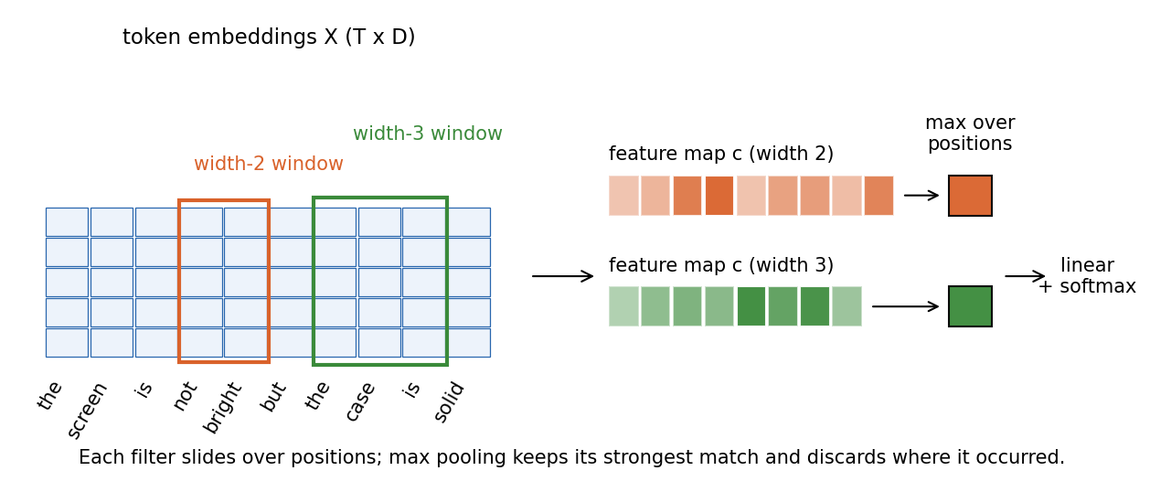
Plain version. A convolutional filter slides along the sentence and fires when it sees a particular short phrase pattern, wherever that pattern occurs. Taking the strongest response of each filter gives a fixed-size summary that remembers which patterns occurred, though not where.
Collobert et al. built a unified neural network for tagging tasks in which convolution over word vectors, followed by max pooling over positions, summarizes a whole sentence [9]. Kim showed that a single convolutional layer on top of pretrained word vectors is a strong sentence classifier [10]. Convolution itself, with its weight sharing and pooling, is developed for images in ML 03; text uses the one-dimensional version, sliding along positions only.
The mathematics of one filter
Stack the token embeddings of a sentence into a matrix whose row is . A filter of width covers consecutive rows:
Here is the window of rows through , contains the filter’s learned weights, sums elementwise products, is a bias, is a nonlinearity such as ReLU or tanh, is the filter’s response at window , the list is the feature map, and is the result of max-over-time pooling. Kim writes the same operation with the window flattened to a vector of length [10].
A model uses many filters. With filters for each width in a set such as , the pooled values form a vector , which a linear layer and softmax turn into class probabilities, trained with cross-entropy as before. In PyTorch, nn.Conv1d(D, F, h) computes all feature maps of width at once; it expects the input as (batch, , ), so the embedding output must be transposed.
What the pieces buy, and what they lose
Weight sharing. The same filter is applied at every position, so a pattern learned from “not good” at the start of one sentence is detected at the end of another. The parameter count depends on , and , not on sentence length.
Soft n-grams. Because the filter takes dot products with embeddings, a filter that responds to “not good” also responds, more weakly, to “not great” if the two adjectives have similar vectors. This is the advantage over sparse bigram features.
Max pooling. Keeping only the maximum handles variable sentence lengths and records whether a pattern occurred anywhere. It discards where the pattern occurred and how many times. A one-layer filter also cannot connect tokens farther apart than its width: with widths up to 4, nothing in the model sees “but” and an adjective four positions later inside the same window. The experiment below shows exactly this.
Kim’s paper compares four ways to treat the embedding table: random initialization trained with the model (CNN-rand), pretrained vectors kept fixed (CNN-static), pretrained vectors fine-tuned (CNN-non-static), and two channels, one fixed and one fine-tuned, with each filter applied to both (CNN-multichannel) [10]. His reported settings use filter widths 3, 4 and 5 with 100 feature maps each, dropout rate 0.5 on the pooled layer, an -norm constraint of 3 on the output weight vectors, and mini-batches of 50 [10]. Zhang and Wallace later ran a sensitivity analysis of this one-layer design and concluded that the filter region size can matter a lot and should be tuned, that 1-max pooling uniformly outperformed the other pooling strategies they tried, that ReLU and tanh were the best activation candidates, and that variance across runs must be reported when comparing configurations [11].
Recurrent encoders take a different route to order: they update a hidden state while reading the sequence and can, in principle, connect distant tokens. Hagiwara’s sentence-classification discussion develops recurrent alternatives alongside practical training [1]. NLP 05 develops them for language and ML 04 gives the shared mathematics. Contextual encoders based on attention let every token’s representation depend on the whole input; NLP 07 and NLP 10 develop them.
Choose according to evidence. A sparse classifier may be enough when labels have clear vocabulary clues. A convolutional or contextual encoder may help with indirect phrasing, negation or domain-specific meanings. Its larger capacity also makes split design and annotation quality more consequential. Complexity should answer a measured failure, such as errors on paraphrases, rather than stand in for evaluation.
Optional: TextCNN (in the Paper guides). Follow the original figure, objective, experimental comparisons and limitations.
Padding, masking and batching
Plain version. Sentences have different lengths, but a batch is a rectangle. We fill short sentences with a padding token and then make sure that padding never influences the result.
Training processes several sequences at once as one tensor of shape (batch, ), where is the longest length in the batch. Shorter sequences are filled with a reserved padding ID, usually 0. A boolean mask records which positions are real:
Here indexes sequences in the batch, indexes positions, is the real length of sequence , is one when its condition holds and zero otherwise, is the embedding at position of sequence , and is the masked mean. The guards against an empty sequence. Each pooling operation needs its own masking rule:
- Mean pooling must divide by the real length, not by . A zero padding vector does not change the sum, but it does change an unmasked denominator.
- Max pooling must exclude padded positions or windows. The general rule is to fill them with before the maximum. After a ReLU, all responses are nonnegative, so filling with 0 is equivalent and has one advantage: a sentence shorter than the filter width, which has no valid window at all, gets 0 instead of , which would turn into NaN in the next layer.
- Convolution windows that overlap padding are not real windows. With right padding, a window of width starting at position is valid exactly when position is real.
- Losses over token positions, used later for tagging and language modeling, must ignore padded positions; PyTorch’s cross-entropy accepts an
ignore_indexfor this.
PyTorch’s nn.Embedding(..., padding_idx=0) keeps the padding row at zero and excludes it from gradient updates. That helps, but it does not make a mean or a max correct by itself. The test is an invariance: adding extra padding must not change any output.
Code · Python · 22 lines
import torch
from torch import nn
from torch.nn import functional as F

torch.manual_seed(0)
emb = nn.Embedding(6, 4, padding_idx=0)            # ID 0 is reserved for padding
seqs = [torch.tensor([3, 5, 2]), torch.tensor([4, 1])]
x = nn.utils.rnn.pad_sequence(seqs, batch_first=True, padding_value=0)
print(x.tolist())                                   # [[3, 5, 2], [4, 1, 0]]

# A lookup is a one-hot row times the table.
one_hot = F.one_hot(x, num_classes=6).float()
assert torch.allclose(one_hot @ emb.weight, emb(x))

def masked_mean(ids):
    mask = (ids != 0).unsqueeze(-1).float()
    return (emb(ids) * mask).sum(1) / mask.sum(1).clamp(min=1)

longer = F.pad(x, (0, 3), value=0)                  # three more padding columns
print("masked mean unchanged:", torch.allclose(masked_mean(x), masked_mean(longer)))
print("plain mean unchanged: ", torch.allclose(emb(x).mean(1), emb(longer).mean(1)))
print("padding row:", emb.weight[0].tolist())
The run prints:
Code · 4 lines
[[3, 5, 2], [4, 1, 0]]
masked mean unchanged: True
plain mean unchanged:  False
padding row: [0.0, 0.0, 0.0, 0.0]
The padding row is zero, yet the plain mean still changes, because its denominator counts padding. Add this kind of invariance check to any new encoder.
Batching has practical consequences beyond correctness. Padding wastes computation, so training code often groups sequences of similar length into the same batch (bucketing). Very long inputs are truncated to a maximum length; record that limit, because text beyond it is invisible to the model, and decide whether to keep the beginning, the end or both. Shuffle batches every epoch so the model does not see the same order of examples, and evaluate with the model in evaluation mode so that dropout is switched off.
Regularization for small text classifiers
Plain version. A neural text model has enough parameters to memorize a small training set, including its labeling mistakes. Regularization makes memorization harder, and a validation set tells us when to stop.
The tools are the general ones from ML 02, applied at specific places in a text model:
- Dropout sets each unit of a layer to zero with probability during training and rescales the rest, so that no unit can rely on a particular partner [12]. In text CNNs it is usually applied to the pooled feature vector, as in Kim’s model [10]. PyTorch’s
nn.Dropout(p)uses the convention that is the probability of dropping a unit. - Word dropout removes entire tokens from the input during training, which encourages the model not to depend on any single word [6].
- Weight decay adds to the loss, the same penalty as in the logistic objective above. The embedding table is often the largest parameter block, so whether it is decayed or frozen matters.
- Max-norm constraints rescale a weight vector whenever its Euclidean norm exceeds a limit, as in Kim’s output layer [10].
- Early stopping keeps the parameters from the epoch with the best validation loss. It is a regularizer too: it limits how far optimization can move toward memorizing the training set.
- Freezing pretrained embeddings removes the largest block of trainable parameters entirely, at the cost of not adapting word meanings to the task.
Every one of these choices is a hyperparameter selected on validation data. Change one at a time and report variation across random seeds before concluding that a choice helps; Zhang and Wallace emphasize exactly this for text CNNs [11].
A complete PyTorch experiment
Plain version. We now compare four classifiers on one invented review task in which order genuinely matters, read their training curves and inspect their mistakes by category.
Each synthetic review is either one clause, “the aspect is (not) adjective,” or two clauses joined by “but.” The label is positive when the deciding clause is positive: a negation flips the adjective, and in a “but” review the second clause decides. Training has 300 reviews with 10% of labels deliberately flipped to imitate annotation noise; validation (300) and test (1,000) labels are clean. Every test review is tagged as plain, negated or contrast so that errors can be counted by category.
Code · Python · 117 lines
import copy, random
import numpy as np
import torch
from torch import nn
from torch.nn import functional as F
from sklearn.feature_extraction.text import TfidfVectorizer
from sklearn.linear_model import LogisticRegression

torch.set_num_threads(1)
ASPECTS = ["battery", "screen", "camera", "speaker", "case", "charger"]
POS, NEG = ["good", "great", "solid", "bright"], ["bad", "weak", "noisy", "dull"]

def clause(rng):
    aspect, positive = rng.choice(ASPECTS), rng.random() < 0.5
    negated = rng.random() < 0.4
    words = ["the", aspect, "is"] + ["not"] * negated + [rng.choice(POS if positive else NEG)]
    return words, int(positive != negated), negated

def example(rng):                       # label of "A but B" is the label of B
    words, label, negated = clause(rng)
    if rng.random() < 0.5:
        second, label, _ = clause(rng)
        return " ".join(words + ["but"] + second), label, "contrast"
    return " ".join(words), label, "negated" if negated else "plain"

def make(n, seed):
    rng = random.Random(seed)
    return [example(rng) for _ in range(n)]

train, val, test = make(300, 1), make(300, 2), make(1000, 3)
flip = random.Random(4)                 # 10% training-label noise; val/test stay clean
train = [(t, 1 - y if flip.random() < 0.1 else y, c) for t, y, c in train]
y_test, kind = np.array([r[1] for r in test]), np.array([r[2] for r in test])

def report(name, pred):
    parts = {k: round(float((pred[kind == k] == y_test[kind == k]).mean()), 3)
             for k in ["plain", "negated", "contrast"]}
    print(f"{name:12s} test acc {np.mean(pred == y_test):.3f}", parts)

for ngrams in [(1, 1), (1, 2)]:
    vec = TfidfVectorizer(ngram_range=ngrams, token_pattern=r"\S+")
    clf = LogisticRegression(C=10.0, max_iter=1000)
    clf.fit(vec.fit_transform([r[0] for r in train]), [r[1] for r in train])
    report(f"tfidf {ngrams}", clf.predict(vec.transform([r[0] for r in test])))

vocab = ["<pad>", "<unk>"] + sorted({w for r in train for w in r[0].split()})
ids = {w: i for i, w in enumerate(vocab)}

def encode(rows):                       # right-pad every sequence with ID 0
    seqs = [torch.tensor([ids.get(w, 1) for w in r[0].split()]) for r in rows]
    return (nn.utils.rnn.pad_sequence(seqs, batch_first=True, padding_value=0),
            torch.tensor([r[1] for r in rows]))

class MeanMLP(nn.Module):               # embedding -> masked mean -> MLP
    def __init__(self, V, D=16, H=32, p=0.3):
        super().__init__()
        self.emb = nn.Embedding(V, D, padding_idx=0)
        self.mlp = nn.Sequential(nn.Linear(D, H), nn.ReLU(), nn.Dropout(p), nn.Linear(H, 2))
    def forward(self, x):
        m = (x != 0).unsqueeze(-1).float()
        return self.mlp((self.emb(x) * m).sum(1) / m.sum(1).clamp(min=1))

class TextCNN(nn.Module):               # embedding -> 1-D conv -> masked max -> linear
    def __init__(self, V, D=16, widths=(2, 3, 4), maps=16, p=0.3):
        super().__init__()
        self.emb = nn.Embedding(V, D, padding_idx=0)
        self.convs = nn.ModuleList(nn.Conv1d(D, maps, h) for h in widths)
        self.drop, self.out = nn.Dropout(p), nn.Linear(maps * len(widths), 2)
    def forward(self, x):
        e, real = self.emb(x).transpose(1, 2), x != 0         # e: (batch, D, T)
        pooled = []
        for conv in self.convs:
            c = torch.relu(conv(e))                           # (batch, maps, T-h+1)
            valid = real[:, conv.kernel_size[0] - 1:].unsqueeze(1)  # window ends on a real token
            # ReLU outputs are >= 0, so filling invalid windows with 0 never wins the max,
            # and a text shorter than the filter gets 0 instead of -inf (which would give NaN).
            pooled.append(c.masked_fill(~valid, 0.0).max(dim=2).values)
        return self.out(self.drop(torch.cat(pooled, dim=1)))

def fit(model, weight_decay, epochs=80, batch=32):
    (xt, yt), (xv, yv) = encode(train), encode(val)
    opt = torch.optim.Adam(model.parameters(), lr=0.01, weight_decay=weight_decay)
    best, history = (float("inf"), None, 0), []
    for epoch in range(1, epochs + 1):
        model.train()
        for b in torch.randperm(len(yt)).split(batch):
            opt.zero_grad()
            F.cross_entropy(model(xt[b]), yt[b]).backward()
            opt.step()
        model.eval()
        with torch.no_grad():
            history.append((F.cross_entropy(model(xt), yt).item(),
                            F.cross_entropy(model(xv), yv).item()))
        if history[-1][1] < best[0]:                          # early stopping on val loss
            best = (history[-1][1], copy.deepcopy(model.state_dict()), epoch)
    model.load_state_dict(best[1])
    return history, best[2]

x_test, _ = encode(test)
for name, build, wd in [("mean+MLP", lambda: MeanMLP(len(vocab)), 1e-4),
                        ("CNN", lambda: TextCNN(len(vocab)), 1e-4),
                        ("CNN no-reg", lambda: TextCNN(len(vocab), p=0.0), 0.0)]:
    torch.manual_seed(0)
    model = build()
    history, best_epoch = fit(model, wd)
    with torch.no_grad():
        pred = model(x_test).argmax(1).numpy()
    print(f"{name:12s} last train/val loss {history[-1][0]:.3f}/{history[-1][1]:.3f}, "
          f"best epoch {best_epoch}")
    report(name, pred)
    if name == "CNN":
        cnn_pred = pred

wrong = np.flatnonzero(cnn_pred != y_test)
print("CNN errors by kind:", {k: int((kind[wrong] == k).sum()) for k in ["plain", "negated", "contrast"]})
for i in wrong[:4]:
    print(" ", y_test[i], "<-", test[i][0])
The whole script runs in a few seconds on one CPU thread and prints:
Code · 13 lines
tfidf (1, 1) test acc 0.546 {'plain': 0.651, 'negated': 0.348, 'contrast': 0.555}
tfidf (1, 2) test acc 0.880 {'plain': 1.0, 'negated': 1.0, 'contrast': 0.77}
mean+MLP     last train/val loss 0.269/0.464, best epoch 36
mean+MLP     test acc 0.797 {'plain': 0.973, 'negated': 0.945, 'contrast': 0.645}
CNN          last train/val loss 0.144/0.431, best epoch 30
CNN          test acc 0.898 {'plain': 0.983, 'negated': 0.945, 'contrast': 0.833}
CNN no-reg   last train/val loss 0.092/0.444, best epoch 10
CNN no-reg   test acc 0.910 {'plain': 1.0, 'negated': 0.928, 'contrast': 0.852}
CNN errors by kind: {'plain': 5, 'negated': 10, 'contrast': 87}
  0 <- the camera is not dull but the battery is weak
  0 <- the camera is noisy but the screen is bad
  1 <- the charger is solid but the battery is solid
  1 <- the charger is solid but the charger is bright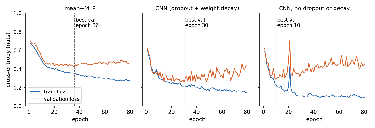
Read the results by category
Unigram TF–IDF fails on negation by construction. In this data, “not” appears equally often in positive and negative reviews, and each adjective is positive or negative depending on whether “not” is present. A linear model over word presence cannot represent that interaction, so negated reviews score 0.348, worse than chance.
Bigrams fix negation, not contrast. The pair “not good” is a single feature, so the bigram model is perfect on plain and negated reviews. On contrast reviews it reaches 0.77: it sees both clauses’ bigrams and has no reliable way to know which clause comes after “but.”
The pooled MLP solves the interaction but not order. Its hidden layer can combine “not” with an adjective, so negated reviews reach 0.945 even though the input is an unordered mean. On contrast reviews it scores 0.645 because mean pooling makes “A but B” and “B but A” identical.
The CNN does best on contrast but is limited by its width. With filters up to width 4 it reaches 0.833 on contrast reviews. All but 15 of its 102 errors are contrast reviews, and the listed errors show why: in “the charger is solid but the battery is solid,” the deciding adjective is four positions after “but,” so no single window contains both. The filters must rely on indirect cues. Exercise 3 asks you to add a width-5 filter and test that explanation.
Read the curves
All three panels show the same pattern: training loss keeps falling while validation loss stops improving and then rises. Training labels contain 10% flipped labels, so a training loss far below that noise level means the model is memorizing mistakes. The unregularized CNN does this fastest: its validation loss bottoms out at epoch 10 and is noticeably worse by epoch 80. Dropout and weight decay slow that drift, and the regularized CNN’s best validation loss comes later.
On test accuracy, however, the unregularized CNN (0.910) and the regularized CNN (0.898) are close once early stopping has chosen each model’s epoch. With one seed and a difference of about one percentage point, this run cannot rank them. The defensible conclusion is narrower: early stopping on a clean validation set is essential here, and the regularized model is less sensitive to when it is stopped. A real comparison would repeat the experiment over several seeds and report the spread [11].
Error analysis as a habit
The category counts were possible only because each test example carried a tag describing why it might be hard. Build such tags into evaluation data from the start: negation, contrast, rare words, length, source. Then read individual errors and ask at which stage the needed evidence was lost. If mean pooling makes two inputs identical, more labels cannot help that model; if the CNN’s windows are too short, a wider filter or a different encoder is the fix; if an annotation is wrong, the fix is in the data.
Evaluate errors and probabilities separately
Plain version. A classifier can choose the right label while giving unreliable probabilities. Evaluate the decision and the uncertainty estimate as different properties.
For one class treated as positive:
Here is precision, is recall, counts true positives, counts false positives, counts false negatives and is their harmonic mean. A zero denominator requires an explicitly chosen convention. Macro F1 averages per-class F1 values equally; support-weighted averaging gives more influence to common classes. The metric documentation specifies these choices [13].
Macro averaging makes failures on a rare category more visible, but it does not encode the actual cost of those failures. Missing an urgent ticket and misrouting a routine receipt can have different consequences. Write a cost policy separately rather than treating a convenient score as a complete utility measure.
Calibration asks whether predicted confidence agrees with observed correctness over comparable examples. A model can preserve its argmax decisions while changing confidence. Guo et al. study this distinction and post-training temperature scaling [14]. Calibration parameters must be fit on held-out development data, with enough samples to estimate probability behavior. Neural classifiers trained to near-zero training loss are a common source of overconfident probabilities, so check calibration whenever the model changes.
For selective prediction:
Here is evaluated-example count, indicates acceptance of example , is its prediction, is its reference label, and is one when its condition holds and zero otherwise. Accepted risk is undefined when no example is accepted. A risk-versus-coverage curve describes the tradeoff over thresholds; choose the deployed threshold using validation rather than final test labels.
Imbalance, error analysis and deployment changes
Plain version. An overall score can improve while an important user group gets worse. Inspect the types of mistakes, the rare classes and the circumstances in which they occur.
Create an error table with text, gold label, predicted label, probability, language, length, source group and an analyst’s explanation. Useful error categories include annotation ambiguity, missing context, negation, unseen vocabulary, multi-topic input, quotation and genuinely out-of-scope text. These categories suggest different repairs. More training examples can help missing vocabulary; they cannot supply a conversation turn that is never available at prediction time.
Class weighting changes how strongly each training example contributes:
Here is weighted cross-entropy, is training-example count, indexes examples, is the document, is its annotated class, is the chosen weight for that class and is the classifier distribution. The weighting policy changes the training objective; it does not manufacture missing linguistic variety.
Weighting, oversampling and threshold changes answer different problems. Weighting changes parameter learning. Oversampling changes the presentation frequency of examples, sometimes repeatedly exposing the same few minority examples. Thresholding changes the action policy after scores are computed. Hagiwara’s development discussion covers imbalance and training choices [1]. Evaluate any intervention on a realistic prevalence distribution rather than on an artificially balanced final test.
Deployment shifts can affect vocabulary, label prevalence and the relationship between text and labels. A new feature release may produce a new technical-error vocabulary; a holiday may increase delivery messages; a changed routing policy may redefine labels. Monitor these separately. A rising fraction of empty feature vectors, or of unknown-word IDs in a neural model, suggests representation coverage; a routing-policy change requires updating the annotation contract.
Keep model and preprocessing artifacts together. The vocabulary order, IDF weights or embedding table, classifier class order, maximum length, probability calibration and decision threshold are a single inference package. Reloading weights with another vocabulary silently changes meanings. Store a versioned label schema and a few deterministic contract examples with the package so that serving can check its assumptions.
Modern view
Survey perspective. Goldberg’s primer organizes neural NLP around feed-forward, convolutional, recurrent and recursive networks, input encoding and computation graphs [5]; it remains a compact map of the models in this lesson. Minaee et al. review more than 150 deep-learning text classifiers and more than 40 datasets, from feed-forward and convolutional models through recurrent, attention-based and pretrained models, and compare reported benchmark results [15]. Read such tables as evidence about specific datasets and protocols, not as a ranking that transfers to an arbitrary label schema.
Zhao et al. organize their LLM survey around pretraining, adaptation, use and evaluation [16]. For classification, this yields a useful comparison among fixed representations with a learned head, task-adapted encoders and instruction-based prediction. Chang et al. organize evaluation by what, where and how to measure [17]. Their perspective warns against treating one familiar benchmark as evidence that an arbitrary label schema works.
Robustness perspective. Sperduti and Moreo’s 2025 misspelling survey reviews sources of spelling variation, correction approaches and the effect on downstream tasks and modern language models [18]. Its practical implication here is to include realistic spelling variation in evaluation, then distinguish normalization failures from classifier failures. Character features, subword embeddings and contextual representations offer different responses; none should be assumed robust without a task-specific comparison.
Practice in 2023–2026. Pretrained Transformer encoders fine-tuned with a classification head, covered in NLP 11, are the usual starting point when labeled data and compute allow. Instruction-following language models broaden the available ways to specify classification tasks [16]. A prompted model can interpret a textual label description without a separately trained classifier head. That shifts part of the configuration into the prompt, label wording and output parser. Treat those artifacts as fitted design choices: fix them before testing, constrain outputs to the allowed schema and measure abstention and malformed responses.
The models in this lesson keep a role. TF–IDF with logistic regression and small convolutional or averaging networks are cheap to train, fast to serve and easy to inspect. They are the baselines that tell you whether a larger model’s gain is real, and they are often adequate when labels have clear lexical cues.
An application can also use a larger model to suggest labels for human review, then train a smaller classifier. This changes the annotation process. Generated labels can contain systematic mistakes or reproduce the teacher’s preferences. Audit a human-checked subset and keep synthetic supervision distinct from independent evaluation labels. The possibility of producing more labels is not proof of better supervision.
Open problems. Label interpretation can drift between annotators and model versions. Low-resource languages may have too little independent evaluation data. Multi-topic messages resist a single-label schema. Calibration can deteriorate after a domain change. Embedding similarity can hide contradiction. These questions need explicit challenge sets and continuing evaluation, not an architecture ranking with all context removed.
Key takeaways
- The annotation contract determines the prediction problem and the available actions; fit vocabulary, IDF weights and any learned representation on training text only.
- A sparse linear baseline is strong, cheap and diagnostic; bigrams capture local negation but treat every phrase as unrelated to every other.
- An embedding layer is a learned lookup table; mean pooling plus a nonlinear MLP can learn word interactions but cannot see order.
- The neural probabilistic language model concatenates learned word vectors and generalizes to unseen histories by sharing evidence between similar words.
- A 1-D convolutional classifier detects soft n-gram patterns anywhere in the text; max pooling discards position, and filter width limits the distance it can connect.
- Padding requires explicit masks for means, maxima, windows and losses; adding padding must not change any output.
- Regularization and early stopping matter most when labels are noisy; compare configurations over several seeds.
- Evaluate class decisions, probability quality, coverage and per-category errors separately.
Exercises
- A label contract. Define a multi-label version of the support task. Write rules for “delivery charge,” a quoted complaint and an empty input. Explain which output activation and loss change.
Hint
Independent label probabilities can allow two routes. Include an explicit rule for when no label is justified rather than interpreting every low score as a negative annotation.
- Train-only features. Introduce a word that occurs only in the final test set. Inspect the fitted TF–IDF vocabulary and transformed test vector, and the ID it receives in the neural experiment’s vocabulary. Compare the result with incorrectly fitting features on all text.
Hint
The correct vocabulary excludes the test-only word; in the neural model it maps to <unk>. Examine document-frequency changes as well as the vocabulary size; leakage can alter weights even when all words already exist.
- Test the width explanation. In the PyTorch experiment, change the CNN’s widths to
(2, 3, 4, 5)and rerun. Does contrast accuracy change? Then run the original and the modified model over five seeds and report mean and range before drawing a conclusion.
Hint
Count the positions in “but the battery is solid.” A width-5 window can contain “but” and the deciding adjective together. Keep everything except the widths fixed, and remember that a single-seed difference can be noise.
- Masking bugs on purpose. Remove the mask from
MeanMLP(use a plain.mean(1)) and fromTextCNN(pool over all windows). Pad the test batch with five extra columns and compare predictions with the masked versions. Which model changes, and why?
Hint
The padding embedding is zero, so a plain mean shrinks toward zero as padding grows. For the CNN, a window that overlaps padding still has a nonzero bias and can win the max.
- A neural language model by hand. For the NPLM with words, history words, features per word and hidden units, count the parameters in , , , , and . Which term dominates when is large, and how does the count change if you remove the direct connections?
Hint
Write the shape of each matrix from the equation. The output layer and the embedding table both scale with ; the hidden layer does not.
- Selective decisions. Run the support-message experiment with several validation cost policies. Plot coverage and accepted error on validation, select one threshold and then evaluate it once on test.
Hint
If no examples are accepted, the accepted-error denominator is zero. Report an undefined value, not perfect accuracy.
References
- M. Hagiwara, Real-World Natural Language Processing: Practical Applications with Deep Learning, Manning, 2021; Chapters 2–4, 7 and 10–11. publisher
- S. McRoy, Principles of Natural Language Processing, open textbook, 2021; Chapter 6, “Benchmark Tasks for Language Modelling.” chapter
- Scikit-learn developers, “Text feature extraction,” scikit-learn documentation, current online edition. documentation
- Scikit-learn developers, “Logistic regression,” scikit-learn documentation, current online edition. documentation
- Y. Goldberg, “A primer on neural network models for natural language processing,” Journal of Artificial Intelligence Research 57, 2016. paper
- M. Iyyer, V. Manjunatha, J. Boyd-Graber and H. Daumé III, “Deep unordered composition rivals syntactic methods for text classification,” ACL-IJCNLP, 2015. paper
- A. Joulin, E. Grave, P. Bojanowski and T. Mikolov, “Bag of tricks for efficient text classification,” EACL, 2017. paper
- Y. Bengio, R. Ducharme, P. Vincent and C. Jauvin, “A neural probabilistic language model,” Journal of Machine Learning Research 3, 2003. paper
- R. Collobert, J. Weston, L. Bottou, M. Karlen, K. Kavukcuoglu and P. Kuksa, “Natural language processing (almost) from scratch,” Journal of Machine Learning Research 12, 2011. paper
- Y. Kim, “Convolutional neural networks for sentence classification,” EMNLP, 2014. paper
- Y. Zhang and B. Wallace, “A sensitivity analysis of (and practitioners’ guide to) convolutional neural networks for sentence classification,” IJCNLP, 2017. paper
- N. Srivastava, G. Hinton, A. Krizhevsky, I. Sutskever and R. Salakhutdinov, “Dropout: a simple way to prevent neural networks from overfitting,” Journal of Machine Learning Research 15, 2014. paper
- Scikit-learn developers, “Classification metrics,” scikit-learn documentation, current online edition. documentation
- C. Guo, G. Pleiss, Y. Sun and K. Q. Weinberger, “On calibration of modern neural networks,” ICML, 2017. paper
- S. Minaee, N. Kalchbrenner, E. Cambria, N. Nikzad, M. Chenaghlu and J. Gao, “Deep learning-based text classification: a comprehensive review,” ACM Computing Surveys 54(3), 2021. survey
- W. X. Zhao et al., “A survey of large language models,” Frontiers of Computer Science, 2026; online manuscript updated March 2026. survey
- Y. Chang et al., “A survey on evaluation of large language models,” ACM Transactions on Intelligent Systems and Technology, 2024. survey
- G. Sperduti and A. Moreo, “Misspellings in natural language processing: a survey,” arXiv:2501.16836, 2025. survey
Check your understanding
This tutorial has 6 exercises. Can you solve them without opening the hints?
Go to the exercises ↑Next NLP 04 · Lexical Semantics and Word Embeddings · 36 min