DLCV 03A・以 YOLOv4 讀懂單階段偵測
先備知識:DLCV 03・物件偵測:從 R-CNN 到 DETR
導覽:本頁與本系列: 導覽:本頁與本系列
本頁內容
- YOLO v1:把偵測當成一次迴歸
- YOLOv2 與 YOLO9000:錨框、先驗與聯合訓練
- YOLOv3:三尺度與 Darknet-53
- SSD:多尺度預設框
- RetinaNet 與 focal loss
- FCOS:逐像素無錨框偵測
- CenterNet:把物件視為點
- YOLOR:顯式特徵與可學隱式表示
- YOLOX:無錨框 YOLO 與 SimOTA
- YOLOv6:重參數化工業偵測器
- YOLOv7:可訓練的免費技巧
- YOLOv9:可編程梯度資訊
- YOLOv10:雙指派的免 NMS 訓練
- YOLOv12:以注意力為核心的 YOLO
- YOLOv13:超圖關聯
- YOLO26:移除 DFL 的端到端 YOLO
- RT-DETR:即時 DETR
- RT-DETRv2:RT-DETR 的實用配方
- D-FINE:逐層精修框分布
- DEIM:密集一對一匹配
- RF-DETR:在 DINOv2 骨幹上搜尋架構
- DEIMv2:為即時 DETR 調適 DINOv3
電腦視覺深度學習
你將學到
- 追蹤 YOLOv4 的輸入、骨幹、頸部、輸出頭與方框解碼。
- 區分只影響訓練,以及影響推論成本的改動。
- 從消融辨認單項效果、交互作用與未測試元件。
- 在註明硬體、精度、輸入大小與計時範圍的條件下比較延遲。
- 透過論文導讀追蹤後續 YOLO 與即時 DETR 的設計變化。
先看全貌
YOLOv4 是一篇研究「配方」的論文:作者整理既有概念與修改,測試哪些訓練、架構技巧適合單張一般 GPU,再組成完整模型。因此骨幹、特徵融合、解碼、指派、增強與後處理都能在同一系統中看清楚;後續方法則提供替代決策。
單階段偵測器適用相機、機器人與工業檢測。YOLOv4 位於這條發展線中段,可藉它理解前代的網格、錨框、多尺度頭,以及後代取代的錨框、NMS、耦合頭。主文詳解 YOLOv4,前後代各有選讀導讀。
先讀 DLCV 03;其核心組件定義框迴歸、IoU、錨框指派、NMS、特徵金字塔與 focal loss。單階段、無錨框、DETR則介紹本章承接的家族。
先看整個家族
白話版。 YOLO 是多個團隊發展的家族;比較結果前,先確認版本、論文與實作。
時間線
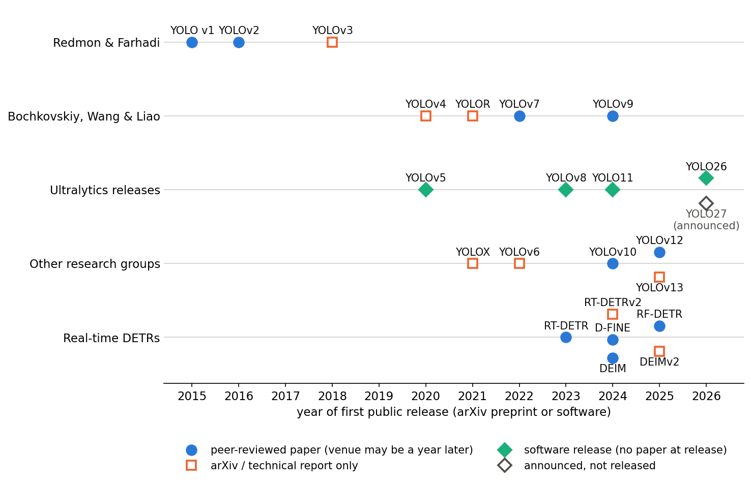
圖 1 依首次公開年份與團隊分類,並標示審查狀態。版本號不是單一血統:YOLOv3 原作者停止後,不同團隊繼續取號;YOLOv4 的其中兩位作者後來提出 v7、v9 [1]、[2]。YOLOv5、v8、YOLO11 是無論文的軟體發行 [3]、[4]、[5]。名稱也無統一管制:2026 年 8 月的「YOLOv14」預印本約兩週後撤回 [6],數字更大本身不代表品質。
本章介紹的論文
下表分為 YOLOv4 前代、後續單階段偵測器、即時 DETR。即時 DETR 的架構不同,但已成為競爭選項;沒有論文的 Ultralytics 發行版放在補充資料。
| 論文 | 年份、場域 | 核心概念 | 對應 YOLOv4 |
|---|---|---|---|
| 前代 | |||
| YOLO v1 [7] | 2016,CVPR | 網格直接迴歸 | 架構 |
| YOLOv2/YOLO9000 [8] | 2017,CVPR | k-means 錨框、有限中心、多尺度訓練 | 頭 |
| YOLOv3 [9] | 2018,技術報告 | 三尺度、Darknet-53、logistic 類別 | 頭 |
| SSD [10] | 2016,ECCV | 多特徵圖預設框 | 架構 |
| RetinaNet [11] | 2017,ICCV | Focal loss 處理前背景不均 | 損失 |
| FCOS [12] | 2019,ICCV | 逐像素框與中心度 | 指派 |
| CenterNet [13] | 2019,arXiv | 物體中心熱圖,不用 IoU NMS | 後處理 |
| 後續方法 | |||
| YOLOR [14] | 2021,arXiv | 與輸入無關的可學隱式張量 | 骨幹 |
| YOLOX [15] | 2021,arXiv | 解耦無錨框頭、SimOTA | 頭 |
| YOLOv6 [16] | 2022,技術報告 | 重參數化、任務對齊、量化 | 骨幹 |
| YOLOv7 [1] | 2023,CVPR | E-ELAN、規劃重參數化、引導標籤 | 完整配方 |
| YOLOv9 [2] | 2024,ECCV | PGI 輔助可逆分支、GELAN | 骨幹 |
| YOLOv10 [17] | 2024,NeurIPS | 一對多/一對一雙指派、免 NMS | 後處理 |
| YOLOv12 [18] | 2025,NeurIPS | 區域注意力 | 注意力 |
| YOLOv13 [19] | 2025,arXiv | 超圖特徵關聯 | 頸部 |
| YOLO26 [20] | 2026,arXiv | 預設免 NMS、移除 DFL、新最佳化器與小物件指派 | 指派 |
| 即時 DETR | |||
| RT-DETR [21] | 2024,CVPR | 混合編碼、不確定性最小查詢 | 後處理 |
| RT-DETRv2 [22] | 2024,技術報告 | 各尺度取樣數、離散取樣 | 配方 |
| D-FINE [23] | 2025,ICLR | 逐層精修框分布 | 損失 |
| DEIM [24] | 2025,CVPR | 密集一對一匹配 | Mosaic |
| RF-DETR [25] | 2026,ICLR | DINOv2 與權重共用架構搜尋 | 骨幹 |
| DEIMv2 [26] | 2025,arXiv | DINOv3 多尺度偵測調適 | 骨幹 |
挑戰
白話版。 YOLOv4 測試既有技巧,希望兼顧準確偵測、即時推論與單張一般 GPU 訓練。
一張一般 GPU 可訓練的快速偵測器
Bochkovskiy、Wang、Liao 於 2020 年 4 月提出 [27]:最準網路常不即時,訓練又需多 GPU、大批次。他們以實際 GPU FPS 定義生產速度,而非只看理論運算量,目標是單張 1080 Ti 或 2080 Ti 即可訓練測試。
YOLOv3 [9] 快,但原表在 僅 33.0% COCO AP [27];EfficientDet [28] 運算量低、準確,卻不必然有高 GPU FPS。YOLOv4 希望兼得兩者優點。
即時的定義與 YOLOv4 計時方式
每幀處理時間短於幀間隔,才有機會即時。延遲是接收一幀到取得最終框的時間,吞吐量是成批處理時每秒完成幾幀。單幀為
含解碼、縮放、正規化、傳輸, 是前向, 含框解碼、閾值與 NMS。 FPS 留下 秒,30 FPS 約 33.3 ms。批次 的吞吐量為 ,但各幀要等整批;即時相機關心批次一延遲。( 以毫秒)轉 FPS 也只適用批次一。
速度表標註「batch=1、無 TensorRT」[29],並依 Maxwell、Pascal、Volta 分組,避免直接混比 GPU [27];30 FPS 以上標為即時。原文未清楚交代精度與是否包含 NMS;後來 YOLOX 以 V100、FP16、batch 1 說明對齊條件 [15]。讀結果時要保留這些限制。
為何測試 freebies 與 specials
許多改進只在特定模型、任務、小資料成立,因此原文將候選分兩袋再測 [27]:
- Bag of freebies(BoF):只改訓練策略或增加訓練成本,推論速度不變,如增強、正規化、平滑、框損失與指派。
- Bag of specials(BoS):增加少量推論成本,換取準確度,如感受野、注意力、特徵融合、啟動與 NMS 變體。
挑戰是找出符合速度與單 GPU 訓練限制的組合。以下依架構、訓練/推論技巧、實驗與未解問題說明。
方法
白話版。 YOLOv4 保留 YOLOv3 頭,加入 CSPDarknet53 與 SPP/PANet 頸部,並整合訓練及推論改良。
偵測器的輸入、骨幹、頸部與頭
白話版。 骨幹把影像變成多尺度特徵,頸部交換各尺度資訊,頭在各格預測框與類別。
原文圖 2、2.1 節整理後續沿用的詞彙 [27]:
- 輸入:影像、區塊或金字塔;YOLOv4 採單張正方形,邊長常為 416、512、608。
- 骨幹:ImageNet [30] 分類預訓練網路;GPU 常用 VGG [31]、ResNet [32] 類,CPU 常採行動骨幹。
- 頸部:連接骨幹與頭,透過 FPN [33]、PAN [34] 等上下路徑整合,SPP [35] 另擴大感受野。
- 頭:密集頭在各位置預測,可有錨框(YOLO、SSD、RetinaNet)或無錨框(CenterNet、FCOS);稀疏頭如兩階段 R-CNN,只處理提案集合。
最終選 CSPDarknet53 [36]、SPP [35]/PAN [34]、YOLOv3 頭 [9]。它是有錨框單階段:三個尺度,每格三錨框,各輸出四框值、一物件度、每類一分數。
正方形邊長 、步幅 8、16、32 時,網格邊長為 ,預測總數為
每格 。 時, 格,共 22,743 預測;416 時為 10,647。每預測 值,COCO 80 類即每尺度 通道,與公開設定一致 [37]。大量候選需閾值與 NMS,因此後處理成本重要。
骨幹:CSPDarknet53
白話版。 骨幹須看得到大物件、容納多物件,且 GPU 上快。原文比較三種後,採 Darknet-53 加跨階段部分連接,讓每階段僅部分通道走昂貴區塊。
3.1 節認為偵測相較分類需更大輸入、更多層與容量,以處理小物件及多尺度。表 1 以 、RTX 2070 比較 [27]:
| 骨幹 | 感受野 | 參數 | BFLOPs | FPS(RTX 2070) |
|---|---|---|---|---|
| CSPResNeXt50 | 425 × 425 | 20.6 M | 31 | 62 |
| CSPDarknet53 | 725 × 725 | 27.6 M | 52 | 66 |
| EfficientNet-B3 [38] | 1311 × 1311 | 12.0 M | 11 | 26 |
EfficientNet-B3 約五分之一運算,FPS 卻不到一半,顯示 FLOPs 不預測 GPU 速度。CSPResNeXt50 分類較佳,CSPDarknet53 偵測較佳,見預訓練消融。後者有 29 個 卷積,前者 16 個,因此感受野較大。
CSP 的作用。 CSPNet [36] 以 DenseNet [39] 說明,也用於 ResNeXt [40] 等。DenseNet 各層接收之前輸出的串接;作者認為部分成本來自重複梯度資訊,這是設計解釋,不是所有層學相同特徵的證明。它將階段輸入分成兩通道群:
表通道串接。只有 經 區塊產生 ,再以 轉換成 ;與未處理的 串接後再轉換:
表卷積, 是轉換權重。分路可減少重複梯度、處理通道與記憶體交通 [36]。「最後融合」先轉區塊輸出再合旁路,可截斷部分重複梯度流且準確度代價小。套到 Darknet-53 即分割、處理、合併的殘差階段。
啟動。 骨幹用 Mish,公開設定的頸部與頭用 LeakyReLU [37]。
頸部一:SPP 區塊
白話版。 多種大小的最大池化,讓最粗圖的一格以低成本看到較大鄰域,再把結果疊為通道。
原始 SPP 用固定長度分類向量 [35],不能原樣放全卷積偵測器。YOLOv4 沿用 YOLOv3 的保尺寸版本:、步幅一、適當填補,再串接 [27]。輸入 時:
是步幅一、same padding 的 池化, 即原圖。608 輸入的步幅 32 圖為 ,13 視窗覆蓋大部分。原文引用 YOLOv3-608 加 SPP 的 AP50 增 2.7%、計算增 0.5%,並指出感受野增加、速度影響小 [27];公開設定有 5、9、13 三池化 [37]。
程式碼 · Python · 16 行
import numpy as np
from scipy.ndimage import maximum_filter

def spp(x, kernels=(5, 9, 13)):
    """YOLO-style SPP. x: (C, H, W). Stride-1 max pooling with 'same' padding keeps H and W;
    the input and the pooled copies are concatenated along the channel axis."""
    pooled = [maximum_filter(x, size=(1, k, k), mode="constant", cval=-np.inf) for k in kernels]
    return np.concatenate([x] + pooled, axis=0)

rng = np.random.default_rng(0)
x = rng.normal(size=(512, 19, 19))          # e.g. the stride-32 map of a 608 x 608 input
print("SPP:", x.shape, "->", spp(x).shape)

one = np.zeros((1, 19, 19)); one[0, 9, 9] = 1.0   # a single strong activation
y = spp(one)
print("cells reached by one activation per group:", [int((g > 0).sum()) for g in y])
輸出
SPP: (512, 19, 19) -> (2048, 19, 19)
cells reached by one activation per group: [1, 25, 81, 169]
通道變四倍,網格仍 ;一個強響應最多影響下一層 格,再以 縮通道。
頸部二:PANet 路徑聚合
白話版。 深層偏語意、淺層偏位置。FPN 向下傳語意,PANet 再向上傳定位。YOLOv4 採雙向頸部,並把相加改為串接。
FPN [33] 以粗圖上採樣加細圖建立 ,見 DLCV 03。PANet [34] 為縮短低層到頂端路徑,另加由下而上增強;原文從 開始:
步幅二 把 尺寸減半,與同尺寸 逐元素相加,再卷積 [34]。YOLOv4 採步幅 8、16、32, 接三頭,取代 YOLOv3 的 FPN [27]。
YOLOv4 修改。 圖 6 把 PAN 相加改為通道串接 再卷積 [27]。保留兩輸入供後層學權重,代價是較多通道。原文列為單 GPU 訓練調整,但未單獨消融相加對串接。
頭:YOLOv3 頭與框解碼
白話版。 每格三模板,各預測位移、伸縮、物件度與類別。YOLOv4 保留頭,但修正中心接近格邊界時難以預測的數值問題。
解碼。 延續 YOLOv2 [8]、YOLOv3 [9]。格左上 以網格為單位,錨寬高 ,輸出 ,框為
, 是網格中心,乘步幅得像素; 是尺寸。物件度為 ,類別各用 sigmoid 與 BCE,可多標籤 [9]。公開九錨框:步幅 8 為 ;16 為 ;32 為 像素 [37]。
網格敏感度。 永不達端點,中心恰在邊界需 ,近邊界也需極大值。原文稱 grid sensitivity,提出乘大於一因子 [27];程式再寫成
為 scale_x_y,偏移 保持範圍居中,可跨格到 [37]。步幅 8、16、32 的 為 1.2、1.1、1.05。程式比較所需 。
程式碼 · Python · 23 行
import numpy as np

sigmoid = lambda t: 1 / (1 + np.exp(-t))
logit = lambda p: np.log(p / (1 - p))

def decode(t, cell, anchor, stride, s=1.0):
    """One YOLOv3/YOLOv4 prediction t = (tx, ty, tw, th) -> box centre and size in pixels.
    s = 1 is the YOLOv3 formula; s > 1 is YOLOv4's grid-sensitivity fix."""
    tx, ty, tw, th = t
    bx = s * sigmoid(tx) - (s - 1) / 2 + cell[0]        # centre in grid units
    by = s * sigmoid(ty) - (s - 1) / 2 + cell[1]
    return bx * stride, by * stride, anchor[0] * np.exp(tw), anchor[1] * np.exp(th)

# cell (10, 7) of the stride-8 grid, anchor 36 x 75 pixels, raw outputs all zero
print("box (cx, cy, w, h):", np.round(decode((0, 0, 0, 0), (10, 7), (36, 75), 8), 1))

# which raw output tx puts the centre at a given position inside its cell?
for pos in (0.5, 0.9, 0.99, 1.0):
    row = []
    for s in (1.0, 1.2):
        p = (pos + (s - 1) / 2) / s                     # the sigmoid value that is needed
        row.append(f"s={s}: " + (f"{logit(p):5.2f}" if p < 1 else "  inf"))
    print(f"centre at {pos:4.2f} of the cell -> tx = " + " | ".join(row))
輸出
box (cx, cy, w, h): [84. 60. 36. 75.]
centre at 0.50 of the cell -> tx = s=1.0:  0.00 | s=1.2:  0.00
centre at 0.90 of the cell -> tx = s=1.0:  2.20 | s=1.2:  1.61
centre at 0.99 of the cell -> tx = s=1.0:  4.60 | s=1.2:  2.29
centre at 1.00 of the cell -> tx = s=1.0: inf | s=1.2: 2.40時,邊界只需 ,不再無限大。消融表的「S」即此,見偵測訓練技巧。
訓練目標。 三項為 CIoU 框損失、物件度 BCE、正樣本類別 BCE。未指派但已高度重疊真值的預測,不必強制當背景;YOLOv3 忽略 IoU 0.5 以上 [9],公開 YOLOv4 ignore_thresh=0.7 [37]。正樣本如何決定見下節。
標籤指派:每物件多個錨框
白話版。 YOLOv3 每物件只給最佳形狀錨框。YOLOv4 保留最佳匹配,再加入夠相似的錨框,增加監督。
YOLOv3 在中心所在格挑形狀 IoU 最高的單錨框 [9]。YOLOv4 先指派最佳,再加符合下式者:
IoU 只比較共中心的寬高, 是閾值。基因搜尋選 ,公開 iou_thresh 相同 [27]、[37]。九錨框跨三尺度,因此可同時在兩層學同一物件;無錨過閾值仍有最佳匹配。完整實作還須處理目標競爭同一預測。
程式碼 · Python · 17 行
import numpy as np

# the nine anchors (width, height in pixels) of yolov4.cfg; three per output stride
anchors = np.array([[12, 16], [19, 36], [40, 28], [36, 75], [76, 55], [72, 146],
                    [142, 110], [192, 243], [459, 401]], float)
stride = np.repeat([8, 16, 32], 3)

def shape_iou(wh, anchors):
    """IoU of boxes that share a centre: only width and height matter."""
    inter = np.minimum(wh[0], anchors[:, 0]) * np.minimum(wh[1], anchors[:, 1])
    return inter / (wh[0] * wh[1] + anchors.prod(1) - inter)

for wh in [(30, 60), (100, 90), (60, 120)]:
    iou = shape_iou(np.array(wh, float), anchors)
    pos = np.union1d([iou.argmax()], np.flatnonzero(iou > 0.213))
    print(f"object {wh[0]:3d}x{wh[1]:<3d} | best anchor {iou.argmax()} (IoU {iou.max():.2f}) | "
          f"IoU > 0.213: anchors {pos.tolist()} on strides {sorted(set(stride[pos].tolist()))}")
輸出
object  30x60  | best anchor 3 (IoU 0.67) | IoU > 0.213: anchors [1, 2, 3, 4] on strides [8, 16]
object 100x90  | best anchor 6 (IoU 0.58) | IoU > 0.213: anchors [3, 4, 5, 6] on strides [16, 32]
object  60x120 | best anchor 5 (IoU 0.68) | IoU > 0.213: anchors [3, 4, 5, 6] on strides [16, 32]
此例每物件由一個變四個正預測,訊號較多,也更需 NMS。消融「IT」即此。後代用當前預測指派,如 YOLOX、YOLOv6,或以一對一免 NMS,如 YOLOv10。DLCV 03另比較兩階段與 RetinaNet。
啟動:Mish
白話版。 YOLOv3 的 LeakyReLU 在零有折角;Mish 平滑、容許小負值,大正值近似恆等,原文發現有助分類與偵測。
Mish 定義為 [41]
。大正值時 ,Mish 近 ;大負值趨零,中間略負而非單調。LeakyReLU 為正側 、其餘 [7]。候選有 ReLU、LeakyReLU、PReLU、ReLU6、SELU、Swish [42]、Mish;原文排除難訓的 PReLU/SELU、偏量化的 ReLU6,並指出 Swish、Mish 連續可微 [27]。
程式碼 · Python · 12 行
import numpy as np

mish = lambda x: x * np.tanh(np.log1p(np.exp(x)))   # x * tanh(softplus(x))
leaky = lambda x: np.where(x > 0, x, 0.1 * x)         # the leaky rectifier of YOLO v1-v3

for v in (-3.0, -1.0, 0.0, 1.0, 3.0):
    print(f"x = {v:4.1f} | Mish {mish(v):7.4f} | leaky {float(leaky(v)):5.2f}")
x = np.linspace(-6, 6, 120001)
i = mish(x).argmin()
print(f"Mish minimum {mish(x[i]):.4f} at x = {x[i]:.3f}")
h = 1e-6
print(f"slope at 0: Mish {(mish(h) - mish(-h)) / (2 * h):.4f}; leaky jumps from 0.1 to 1")
輸出
x = -3.0 | Mish -0.1456 | leaky -0.30
x = -1.0 | Mish -0.3034 | leaky -0.10
x =  0.0 | Mish  0.0000 | leaky  0.00
x =  1.0 | Mish  0.8651 | leaky  1.00
x =  3.0 | Mish  2.9865 | leaky  3.00
Mish minimum -0.3088 at x = -1.192
slope at 0: Mish 0.6000; leaky jumps from 0.1 to 1
Mish 零點斜率 0.6,LeakyReLU 則由 0.1 跳到 1;最小值約 ,超過 3 接近恆等。原文 CSPResNeXt-50 分類 top-1 77.9%→78.9%,Mish 預訓練 CSPDarknet53 的偵測最佳 [27];代價是比整流多運算。
框損失:從 IoU 到 CIoU
白話版。 分開算四座標誤差,忽略它們共同描述一個框。IoU 衡量重疊,CIoU 再加中心距離與長寬比。
原文回顧 [27]:未正規化座標平方差受單位影響。UnitBox 用 [43];常見 在零重疊仍有限、共同縮放不變,但框分離時梯度為零。GIoU [44] 加最小包圍框懲罰,DIoU/CIoU [45] 再加中心距離與比例。對預測 、真值 :
為中心, 為歐氏距離, 為最小包圍框對角長, 為寬高, 為比例差, 讓重疊佳時比例項更重要 [45]。去末項為 DIoU,再去距離為 IoU。DLCV 03有四者比較;以下拆解 CIoU 三項。
程式碼 · Python · 21 行
import numpy as np

def iou_terms(a, b):
    """a, b: boxes (x1, y1, x2, y2). Returns IoU, the DIoU penalty rho^2/c^2 and the CIoU term alpha*v."""
    iw = max(0.0, min(a[2], b[2]) - max(a[0], b[0])); ih = max(0.0, min(a[3], b[3]) - max(a[1], b[1]))
    inter = iw * ih
    wa, ha, wb, hb = a[2] - a[0], a[3] - a[1], b[2] - b[0], b[3] - b[1]
    iou = inter / (wa * ha + wb * hb - inter)
    cw = max(a[2], b[2]) - min(a[0], b[0]); ch = max(a[3], b[3]) - min(a[1], b[1])
    rho2 = ((a[0] + a[2] - b[0] - b[2]) ** 2 + (a[1] + a[3] - b[1] - b[3]) ** 2) / 4
    v = 4 / np.pi ** 2 * (np.arctan(wb / hb) - np.arctan(wa / ha)) ** 2
    alpha = v / ((1 - iou) + v) if v > 0 else 0.0
    return iou, rho2 / (cw ** 2 + ch ** 2), alpha * v

gt = (100, 100, 200, 300)                                  # 100 x 200 pixels, tall
preds = {"centred, lying flat":       (50, 150, 250, 250),
         "shifted, right shape":      (125, 125, 225, 325),
         "far away":                  (300, 100, 400, 300)}
for name, p in preds.items():
    iou, d, av = iou_terms(p, gt)
    print(f"{name:26s} IoU {iou:.3f} | L_IoU {1 - iou:.3f} | L_DIoU {1 - iou + d:.3f} | L_CIoU {1 - iou + d + av:.3f}")
輸出
centred, lying flat        IoU 0.333 | L_IoU 0.667 | L_DIoU 0.667 | L_CIoU 0.700
shifted, right shape       IoU 0.488 | L_IoU 0.512 | L_DIoU 0.530 | L_CIoU 0.530
far away                   IoU 0.000 | L_IoU 1.000 | L_DIoU 1.308 | L_CIoU 1.308
同中心錯比例只有比例懲罰,同形狀位移只有距離懲罰;遠框 IoU 為零,但距離仍提供方向。YOLOv4 認為 CIoU 收斂與準確較佳 [27],公開 iou_loss=ciou、iou_normalizer=0.07 [37]。
後處理:NMS 與 DIoU-NMS
白話版。 多個正樣本會重複預測同一物件,NMS 留最佳、刪高度重疊者,成本依場景而變。DIoU-NMS 降低中心相隔較遠的框被誤刪的機會。
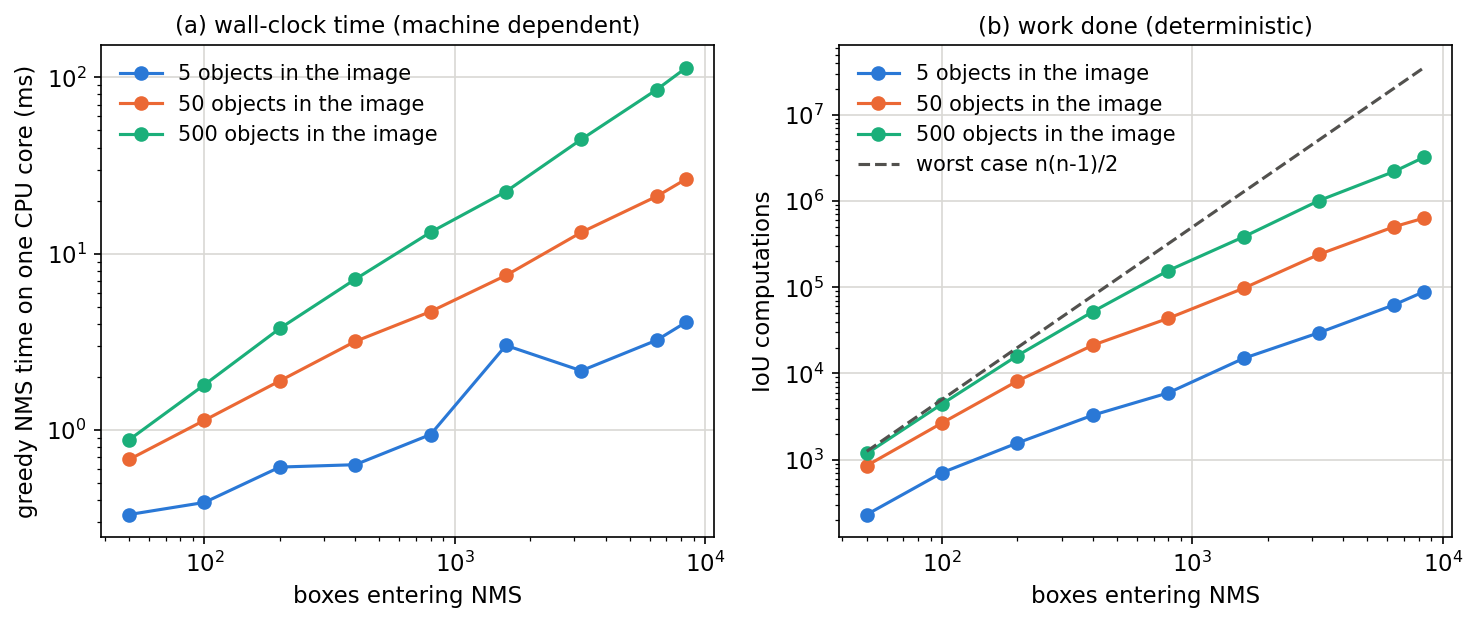
貪婪 NMS。 DLCV 03定義:先取最高分,與剩餘框算 IoU、刪過閾值者、重複。 候選若很少被刪,比較數接近
是每次保留後的剩餘框數。若多為少數物件的重複框,會早刪而省工。因此成本依候選數、信心閾值與場景,不像固定形狀網路前向較穩定。範例的比較次數確定,時間則隨機器變。
程式碼 · Python · 32 行
import numpy as np

def nms_count(boxes, scores, thr=0.5):
    """Greedy NMS that also counts how many box-pair IoUs it computes."""
    order = np.argsort(-scores)
    keep, n_iou = [], 0
    while order.size:
        i, rest = order[0], order[1:]
        keep.append(i)
        n_iou += rest.size
        x1 = np.maximum(boxes[i, 0], boxes[rest, 0]); y1 = np.maximum(boxes[i, 1], boxes[rest, 1])
        x2 = np.minimum(boxes[i, 2], boxes[rest, 2]); y2 = np.minimum(boxes[i, 3], boxes[rest, 3])
        inter = np.clip(x2 - x1, 0, None) * np.clip(y2 - y1, 0, None)
        area = lambda b: (b[..., 2] - b[..., 0]) * (b[..., 3] - b[..., 1])
        iou = inter / (area(boxes[i]) + area(boxes[rest]) - inter)
        order = rest[iou <= thr]
    return len(keep), n_iou

def random_boxes(n, n_objects, rng, size=640):
    """n candidate boxes jittered around n_objects true objects."""
    centres = rng.uniform(40, size - 40, (n_objects, 2))
    owner = rng.integers(0, n_objects, n)
    c = centres[owner] + rng.normal(0, 6, (n, 2))
    wh = rng.uniform(30, 60, (n, 2))
    return np.hstack([c - wh / 2, c + wh / 2]), rng.random(n)

rng = np.random.default_rng(0)
for n_objects in (5, 500):                       # few objects vs a crowded scene
    for n in (100, 1000, 8400):
        b, s = random_boxes(n, n_objects, rng)
        kept, n_iou = nms_count(b, s)
        print(f"objects {n_objects:3d} | boxes {n:4d} | kept {kept:4d} | IoUs {n_iou:9,d}")
輸出
objects   5 | boxes  100 | kept   21 | IoUs       770
objects   5 | boxes 1000 | kept   43 | IoUs     7,809
objects   5 | boxes 8400 | kept   86 | IoUs    90,699
objects 500 | boxes  100 | kept   94 | IoUs     4,621
objects 500 | boxes 1000 | kept  513 | IoUs   209,490
objects 500 | boxes 8400 | kept 1259 | IoUs 3,039,292
同為 8,400 候選,擁擠例需要約 34 倍 IoU 比較。GPU 最佳化與候選上限會改時間,因此這只是教學分析,不是部署預測。圖 2 掃候選數;YOLOv10、RT-DETR移除這項成本,後者也在真偵測器量測。
DIoU-NMS。 單靠 IoU 可能把相鄰兩人當重複,DIoU 在判斷前減中心距離項 [45]:
是框 分數,零表示刪除; 為中心 距離, 為包圍框對角, 是閾值。中心較遠的框較容易留下 [45]。YOLOv4 列為 detector BoS [27],程式可獨立執行。
程式碼 · Python · 27 行
import numpy as np

def iou_terms(a, b):
    """a, b: boxes (x1, y1, x2, y2). Returns IoU, the DIoU penalty rho^2/c^2 and the CIoU term alpha*v."""
    iw = max(0.0, min(a[2], b[2]) - max(a[0], b[0])); ih = max(0.0, min(a[3], b[3]) - max(a[1], b[1]))
    inter = iw * ih
    wa, ha, wb, hb = a[2] - a[0], a[3] - a[1], b[2] - b[0], b[3] - b[1]
    iou = inter / (wa * ha + wb * hb - inter)
    cw = max(a[2], b[2]) - min(a[0], b[0]); ch = max(a[3], b[3]) - min(a[1], b[1])
    rho2 = ((a[0] + a[2] - b[0] - b[2]) ** 2 + (a[1] + a[3] - b[1] - b[3]) ** 2) / 4
    v = 4 / np.pi ** 2 * (np.arctan(wb / hb) - np.arctan(wa / ha)) ** 2
    alpha = v / ((1 - iou) + v) if v > 0 else 0.0
    return iou, rho2 / (cw ** 2 + ch ** 2), alpha * v


def nms(boxes, scores, thr=0.5, diou=False):
    order, keep = list(np.argsort(-scores)), []
    while order:
        m = order.pop(0); keep.append(int(m))
        crit = lambda j: iou_terms(boxes[m], boxes[j])[0] - (iou_terms(boxes[m], boxes[j])[1] if diou else 0)
        order = [j for j in order if crit(j) < thr]
    return keep

# two people side by side (centres 32 px apart) and one duplicate of the first person
boxes = np.array([[100, 100, 200, 200], [132, 100, 232, 200], [103, 100, 203, 200]], float)
scores = np.array([0.9, 0.8, 0.7])
print("greedy NMS keeps:", nms(boxes, scores), "| DIoU-NMS keeps:", nms(boxes, scores, diou=True))
輸出
greedy NMS keeps: [0] | DIoU-NMS keeps: [0, 1]第二人 IoU 0.515 略過閾值,貪婪 NMS 刪除;減距離後 0.478,DIoU-NMS 保留,中心僅差三像素的重複框仍刪。效果只在部分重疊範圍,無法解所有擁擠歧義,原消融也未單獨量它。
資料增強:Mosaic 與 CutMix
白話版。 Mosaic 拼四圖,讓每個訓練畫面含不同背景與較小物件,是 YOLOv4 最廣為沿用的技巧。
原文整理光度、縮放、裁切、翻轉、旋轉與遮擋,也比較 MixUp [46] 的像素/標籤加權,及 CutMix [47] 的矩形貼上與面積混標籤。骨幹分類用 CutMix,偵測引入四圖 Mosaic;致謝 Glenn Jocher 提供 Mosaic、基因搜尋與網格修正概念 [27]。
原文理由:物件出現於非典型背景,且一張拼圖的 BN 統計來自四圖,可降低大批次需求 [27],呼應單 GPU 目標。
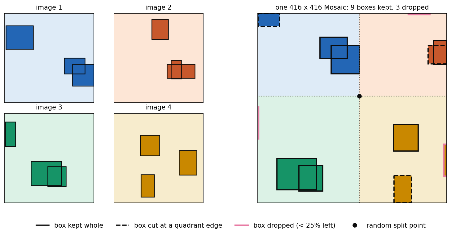
原文只以圖 3 說明,縮放裁切依實作不同。以下示例選隨機分割點,讓四圖角落相接,裁掉各象限外區域,再裁切或丟棄框。
程式碼 · Python · 40 行
import numpy as np

def mosaic(images, boxes, size=416, rng=None, min_keep=0.25):
    """Place four images around a random split point (xc, yc) of a size x size canvas.
    images: four (H, W, 3) arrays; boxes: four (n, 4) arrays of (x1, y1, x2, y2) in pixels.
    Each image touches the split point with one corner; whatever falls outside its quadrant is cut.
    A box is kept if at least `min_keep` of its area survives the cut."""
    xc, yc = (int(v) for v in rng.uniform(0.3, 0.7, 2) * size)
    canvas = np.full((size, size, 3), 114, np.uint8)
    out, n_cut, n_drop = [], 0, 0
    for k, (img, bx) in enumerate(zip(images, boxes)):
        h, w = img.shape[:2]
        ox = xc - w if k in (0, 2) else xc          # where the image's top-left corner lands
        oy = yc - h if k in (0, 1) else yc
        rx0, rx1 = (0, xc) if k in (0, 2) else (xc, size)   # the quadrant it may fill
        ry0, ry1 = (0, yc) if k in (0, 1) else (yc, size)
        x0, x1, y0, y1 = max(rx0, ox), min(rx1, ox + w), max(ry0, oy), min(ry1, oy + h)
        canvas[y0:y1, x0:x1] = img[y0 - oy:y1 - oy, x0 - ox:x1 - ox]
        shifted = bx + [ox, oy, ox, oy]
        clipped = np.clip(shifted, [x0, y0, x0, y0], [x1, y1, x1, y1])
        area = lambda b: (b[:, 2] - b[:, 0]) * (b[:, 3] - b[:, 1])
        keep = area(clipped) >= min_keep * area(shifted)
        n_cut += int((keep & (area(clipped) < area(shifted))).sum()); n_drop += int((~keep).sum())
        out.append(clipped[keep])
    return canvas, np.concatenate(out), (xc, yc), n_cut, n_drop

rng = np.random.default_rng(0)
imgs, bxs = [], []
for k in range(4):                                   # four synthetic 256 x 256 "photos"
    img = np.full((256, 256, 3), 60 * k + 40, np.uint8)
    b = []
    for _ in range(3):                               # three rectangles = three objects each
        x, y = rng.integers(0, 200, 2); w, h = rng.integers(30, 90, 2)
        x2, y2 = min(x + w, 256), min(y + h, 256)
        img[y:y2, x:x2] = rng.integers(0, 256, 3); b.append([x, y, x2, y2])
    imgs.append(img); bxs.append(np.array(b, float))

canvas, boxes, split, n_cut, n_drop = mosaic(imgs, bxs, rng=rng)
print("canvas", canvas.shape, "| split point", split)
print(f"objects in: {sum(len(b) for b in bxs)} | kept: {len(boxes)} (of which cut: {n_cut}) | dropped: {n_drop}")
輸出
canvas (416, 416, 3) | split point (223, 181)
objects in: 12 | kept: 9 (of which cut: 3) | dropped: 3
圖 3 中十二物件有三個只剩部分、三個幾乎全被裁。此處剩不到四分之一面積就丟,是教學實作選擇,非原文規則。後來 DEIM 另用 Mosaic 增加每圖物件,給一對一更多正樣本。
自對抗訓練
白話版。 SAT 先固定權重、改影像讓偵測器受騙,再正常訓練辨識改過的圖,是偵測器自己生成的增強。
原文描述兩次前反向:先對自己做攻擊,使期望物件難以被看見,再在修改圖上正常訓練 [27]。以下是本章示意,不是原文精確公式:
為影像與框標籤, 為偵測器, 為損失, 為影像變化量, 為學習率。第一步固定權重、提高所選目標;一般偵測損失上升也可能只是定位變差,不一定隱藏物件。第二步正常訓練。SAT 增加訓練計算,不改推論;原文沒有單獨量時間,也無 SAT 消融欄,見證據限制。
正規化:DropBlock 與標籤平滑
白話版。 正規化刻意讓訓練困難,減少記憶資料。DropBlock 關掉整塊特徵,標籤平滑則避免對類別過度確信。
Dropout [48] 獨立歸零,但相鄰卷積特徵高度相關,容易從鄰居補回。DropBlock [49] 在能放完整 區塊的位置抽 Bernoulli 種子,再歸零整塊、乘遮罩,依總位置數/保留數重縮放。 特徵欲丟約 ,種子率為
是保留率, 是區塊邊長, 是特徵邊長, 為合法種子數;區塊會重疊,故為近似 [49]。原文還由保留率一逐漸降到目標,避免早期傷害。
程式碼 · Python · 21 行
import numpy as np

def dropblock_mask(feat, block, keep_prob, rng):
    """One DropBlock mask for a feat x feat map (Ghiasi et al., Algorithm 1)."""
    gamma = (1 - keep_prob) / block ** 2 * feat ** 2 / (feat - block + 1) ** 2
    half = block // 2
    seeds = np.zeros((feat, feat), bool)                       # only where a whole block fits
    seeds[half:feat - half, half:feat - half] = rng.random((feat - block + 1,) * 2) < gamma
    mask = np.ones((feat, feat))
    for i, j in zip(*np.nonzero(seeds)):
        mask[i - half:i + half + 1, j - half:j + half + 1] = 0.0
    return mask, gamma

rng = np.random.default_rng(0)
feat, block, keep = 38, 7, 0.9
masks = [dropblock_mask(feat, block, keep, rng)[0] for _ in range(2000)]
gamma = dropblock_mask(feat, block, keep, rng)[1]
dropped = 1 - np.mean([m.mean() for m in masks])
print(f"gamma = {gamma:.5f} | target drop rate {1 - keep:.2f} | measured {dropped:.3f}")
m = masks[0]
print("first mask: dropped units", int((m == 0).sum()), "| rescale factor", round(m.size / m.sum(), 3))
輸出
gamma = 0.00288 | target drop rate 0.10 | measured 0.094
first mask: dropped units 171 | rescale factor 1.134、 區塊,種子率不到 0.3% 就丟約 9.4%,因重疊略低於 10% 目標。YOLOv4 把它列在骨幹及偵測 BoF,但未單獨消融 [27]。
類別標籤平滑。 硬 one-hot 的交叉熵持續提高正確 logit,可能過度確信;平滑改為 [50]
索引 類, 為真類, 是相等指示, 為平滑量。YOLOv4 用獨立 sigmoid,LS 欄指 sigmoid 平滑 [27];二元情況可令 ,正負目標變 ,原文未給 。分類 top-1 77.9%→78.1%,但單獨用於偵測 AP 38.0%→33.0%,見消融。
正規化:跨迷你批次 CmBN
白話版。 單 GPU 每次只放少量圖,BN 統計不穩。CmBN 在同一次權重更新的多個迷你批次間累積統計。
BN [51] 為 ; 是啟動, 是當批均值變異數, 可學, 防除零。4 或 8 張統計較吵。CBN [52] 跨迭代,但權重改變,須用 Taylor 近似修正舊統計;跨 GPU 同步則不解單卡限制。
YOLOv4 批次 64,分成 8 或 4 張的 subdivisions,整批才更新 [27]、[37]。CmBN 只跨同批迷你批次。依圖 4,可示意第 個累積前 個:
是等大迷你批次,變異數為母體動差。只平均變異數會漏掉批次均值差;同批權重不變,所以不需跨更新補償。此為正確動差聚合示例,不是原文公式或完整程式規格。CBN 欄單獨 AP 38.4%,基準 38.0% [27]。
注意力與融合:改良 SAM 與加權殘差
白話版。 注意力重加權特徵。YOLOv4 簡化 CBAM 的空間注意力為逐元素閘門,另列 EfficientDet 的可學加權相加。
CBAM 的 SAM [53] 對 沿通道取平均與最大,串成兩張圖再卷積:
為卷積, 為 sigmoid, 跨通道廣播相乘。原文估 SAM 額外計算約 0.1%、GPU 速度幾乎不變,相較代表性通道注意力約增 10% 時間 [27]。圖 5 改成直接卷積 ,閘門同形狀、逐元素縮放。CSPResNeXt50-PANet-SPP 加 SAM,AP 42.4%→42.7%。
多輸入加權殘差 MiWRC。 EfficientDet 用非負可學權重做快速正規化融合 [28]:
是輸入圖, 由 ReLU 保證, 防除零 [28]。YOLOv4 列為骨幹 BoS,未單獨量貢獻。
訓練排程:餘弦退火、基因搜尋與隨機尺寸
白話版。 有些技巧只改學習率、超參數選法與訓練輸入尺寸,不改推論網路。
SGDR [54] 讓學習率沿半個餘弦下降:
是上下界, 是重啟後 epoch, 是週期長。YOLOv4 的 CA 單用 AP 38.7%,階梯基準 38.0% [27]。
基因搜尋 GA。 短訓多組參數,保留較佳者,再突變、組合。原文用前 10% 時段搜尋;YOLOv3-SPP、GIoU、5,000 圖 min-val、300 epochs,選出學習率 0.00261、動量 0.949、指派閾值 0.213、框損失正規化 0.07。GA 單獨 AP 38.9%,基準 38.0% [27]。
隨機形狀與動態批次。 延續 YOLOv2 多尺度 [8],改訓練解析度,使一模型支援多尺寸。DM 在小圖自動加迷你批次以滿載 GPU,但單獨 AP 降至 35.3% [27]。
最佳化錨框 OA。 依 重新估錨形狀,延續 YOLOv2 的 IoU k-means,見 DLCV 03 補充資料 [27]。
完整配方
白話版。 CSPDarknet53+SPP+PAN+YOLOv3 頭,再搭訓練技巧與少量推論模組。
原文 3.4 節列為 [27]:
| 部位 | 使用項目 | 類型 |
|---|---|---|
| 骨幹 | CSPDarknet53 | 架構 |
| 頸部 | SPP、串接版 PAN | 架構 |
| 頭 | YOLOv3,三尺度各三錨框 | 架構 |
| 骨幹 BoF | CutMix、Mosaic、DropBlock、標籤平滑 | 訓練 |
| 骨幹 BoS | Mish、CSP、MiWRC | 推論有成本 |
| 偵測 BoF | CIoU、CmBN、DropBlock、Mosaic、SAT、網格修正、多錨框、餘弦退火、基因搜尋、隨機尺寸 | 訓練 |
| 偵測 BoS | Mish、SPP、改良 SAM/PAN、DIoU-NMS | 推論有成本 |
後代保留整體形狀,替換個別決策;問題對照這些替換。
結果
白話版。 YOLOv4 在 COCO、608 輸入達 43.5% AP;416 版本在三種 GPU 世代都超過 30 FPS,但 608 在 Maxwell 只有 23 FPS。原比較依速度與準確度取捨,而非全尺寸皆即時。
訓練與評估設定
偵測在 COCO [55] 訓練、test-dev 2017 報 AP [56]:IoU 0.50–0.95 平均、AP50、AP75、小中大物件。分類則 ImageNet [30] 訓練、ILSVRC 2012 驗證 [27]。
偵測預設 500,500 步,學習率 0.01,400,000、450,000 步各乘 0.1,動量 0.9、衰減 0.0005;單 GPU、多尺度、批次 64、迷你批次 8 或 4。分類預設 8,000,000 步、批次 128/迷你 32、0.1 多項式衰減、1,000 暖身、動量 0.9、衰減 0.005;分類 BoF 多訓 50%,皆單張 1080 Ti 或 2080 Ti [27]。
主要比較
表 8、9、10 按 Maxwell、Pascal、Volta 分開不同顯卡,皆 batch 1、無 TensorRT [27]。YOLOv4 準確度相同,只重新測速度:
| 輸入 | AP | AP50 | AP75 | APS | APM | APL | FPS Maxwell | FPS Pascal | FPS Volta |
|---|---|---|---|---|---|---|---|---|---|
| 416 | 41.2 | 62.8 | 44.3 | 20.4 | 44.4 | 56.0 | 38 | 54 | 96 |
| 512 | 43.0 | 64.9 | 46.5 | 24.3 | 46.1 | 55.2 | 31 | 43 | 83 |
| 608 | 43.5 | 65.7 | 47.3 | 26.7 | 46.7 | 53.3 | 23 | 33 | 62 |
與其他列比較時:
- Maxwell 上 YOLOv3-608 AP 33.0%、SPP 36.2%,皆 20 FPS;YOLOv4-608 約增十個 AP 百分點且略快 [27]。
- Volta 上 EfficientDet-D0 至 D3 AP 33.8、39.6、43.0、45.8%,FPS 62.5、50.0、41.7、23.8。YOLOv4-512 同為 43.0% 卻 83 FPS;D3 更準但低於 30 FPS。這是相近準確度約快兩倍的依據 [27]。
- 表 9 更慢方法最高 46.8% AP/1.3 FPS;YOLOv4 並非宣稱全體最高 AP,而是即時範圍的取捨 [27]。
大物件 AP 隨輸入增大 56.0→55.2→53.3,小物件則 20.4→26.7;更大解析度並非各尺度都得利。摘要說 V100 約 65 FPS,表 10 卻列 62 FPS [27],應採較明確表值。
速度:量測檢查清單
讀取或量測任何偵測延遲,應核對:
- 硬體、引擎、精度一致。 YOLOv4 有 GPU 世代與無 TensorRT,未明確精度。
- 批次一。 大批次吞吐不能直接代表相機延遲。
- 端到端邊界。 包含前處理、網路、NMS 等後處理,或清楚列排除。YOLOv4 未明確 NMS;RT-DETR、YOLOv10則在 COCO 圖片平均計入。
- 同裝置。 同 GPU 世代不等於同卡;競爭列來自各論文,小 FPS 差不能視為同硬體測量。
- 暖身與平均。 排除記憶體配置、核心選擇的初期時間,再平均多張。
- 輸入與閾值。 NMS 候選取決於信心閾值,低閾值算 AP 也會改時間。
消融實驗
白話版。 原文先測分類骨幹、再測偵測 BoF/BoS、骨幹權重與批次。逐列閱讀才能分清強證據與尚未隔離的項目。
分類器消融
表 2、3 比較 ImageNet 的技巧、啟動與 top-1/top-5 [27]。
| CSPResNeXt-50 設定 | Top-1 | Top-5 |
|---|---|---|
| 基準 | 77.9 | 94.0 |
| MixUp | 77.2 | 94.0 |
| CutMix | 78.0 | 94.3 |
| Mosaic | 78.1 | 94.5 |
| 雙邊模糊 | 77.5 | 93.8 |
| 標籤平滑 | 78.1 | 94.4 |
| Swish | 64.5 | 86.0 |
| Mish | 78.9 | 94.5 |
| CutMix+Mosaic+平滑 | 78.5 | 94.8 |
| 再加 Mish | 79.8 | 95.2 |
CSPDarknet-53 基準 77.2/93.6,三技巧 77.8/94.4,再加 Mish 78.7/94.8 [27]。這支持該設定的組合,MixUp、模糊未改善。Swish 64.5% 異常低而原文未解釋,不應泛化為 Swish 本質差。
偵測器的訓練技巧
表 4 在 、CSPResNeXt50-PANet-SPP 測 S 網格修正、M Mosaic、IT 多錨框、GA 搜尋、LS 平滑、CBN、CA 餘弦、DM 動態批次、OA 錨框與損失 [27]。
| 類別 | 設定 | AP | AP50 | AP75 |
|---|---|---|---|---|
| 基準 | MSE、無技巧 | 38.0 | 60.0 | 40.8 |
| 單項、MSE | S | 37.7 | 59.9 | 40.5 |
| M | 39.1 | 61.8 | 42.0 | |
| IT | 36.9 | 59.7 | 39.4 | |
| GA | 38.9 | 61.7 | 41.9 | |
| LS | 33.0 | 55.4 | 35.4 | |
| CBN | 38.4 | 60.7 | 41.3 | |
| CA | 38.7 | 60.7 | 41.9 | |
| DM | 35.3 | 57.2 | 38.0 | |
| S+損失 | GIoU/DIoU/CIoU | 39.4/39.1/39.6 | 59.4/58.8/59.2 | 42.5/42.1/42.6 |
| 組合 | S+M+IT+GA、CIoU | 41.5 | 64.0 | 44.8 |
| M+GA+OA、CIoU | 36.1 | 56.5 | 38.4 | |
| S+M+IT+GA+OA、MSE | 40.3 | 64.0 | 43.1 | |
| 同組合、GIoU | 42.4 | 64.4 | 45.9 | |
| 同組合、CIoU | 42.4 | 64.4 | 45.9 |
表格支持以下觀察:
- Mosaic 單用增 1.1 AP 最多,GA、CA、CmBN 也有小增益。
- IoU 類優於 MSE;搭 S 時 CIoU 39.6 略高於 GIoU 39.4,最佳組合兩者同為 42.4。
- S、IT、DM、LS 單獨分別降 0.3、1.1、2.7、5.0 AP,但 S、IT 出現在佳組合。需更強訓練才能利用新增正樣本是合理解釋,非原文已分析結論。
- 最佳列沒有 LS、CBN、CA、DM,雖最終清單列部分項目;表內沒有全部 BoF 一起啟用的列。
偵測器的推論模組
表 5 基礎 SPP/PAN 42.4% AP,加 SAM 42.7%(AP50 64.6、AP75 46.3);其他感受野、高斯不確定性頭、自適應融合組合降至 41.1–41.8% [27]。更多模組未必好;DIoU-NMS、偵測 Mish、MiWRC 沒有獨立列。
骨幹與預訓練權重
表 6 在相近設定、512 輸入比較初始化 [27]:
| 骨幹與分類初始化 | AP | AP50 | AP75 |
|---|---|---|---|
| CSPResNeXt50,預設 | 42.4 | 64.4 | 45.9 |
| CSPResNeXt50,BoF | 42.3 | 64.3 | 45.7 |
| CSPResNeXt50,BoF+Mish | 42.3 | 64.2 | 45.8 |
| CSPDarknet53,BoF | 42.4 | 64.5 | 46.0 |
| CSPDarknet53,BoF+Mish | 43.0 | 64.9 | 46.5 |
CSPResNeXt50 分類 77.9→79.8% 不帶來較佳偵測,CSPDarknet53 卻有幫助。這支持骨幹選擇,也顯示分類準確度不是可靠偵測代理。
迷你批次大小
表 7 未加技巧時,608 CSPResNeXt50 以迷你 4/8 得 37.1/38.4 AP;完整 512 CSPDarknet53 得 41.6/41.7 [27]。該設定下批次影響變小,支持單卡可訓。Mosaic、CmBN 為此設計,但本表未隔離兩者貢獻。
結論
YOLOv4 展示有錨框單階段偵測,可透過骨幹、頸部與測試過的技巧,在速度及準確度取得實用折衷、單張消費 GPU 訓練。Mosaic、IoU 損失、搜尋、正樣本、SPP、PAN、SAM 有不同程度實驗支持;有些流行技巧無效,最佳分類骨幹也未必最佳偵測。持久貢獻是組件詞彙與在偵測本身驗證配方的做法。
問題
白話版。 錨框、共用頭、多正樣本與 NMS 都是後代改進點。證據也有限:部分組件未測、消融單次且使用 test-dev,原論文未經同儕審查。
方法限制
- 錨框依資料。 COCO 的九模板未必適合新資料與尺寸,YOLOX因此移除。
- 耦合頭。 分類定位共用卷積;YOLOX 顯示解耦可加速收斂。
- 固定指派。 形狀與中心規則不看目前預測,後來有 SimOTA、YOLOv6 的任務對齊。
- 依賴 NMS。 有閾值、場景相依成本與鄰近物件誤刪;YOLOv10提供免 NMS 路線。
- 高解析度大物件。 APL 在 416、608 分別 56.0、53.3 [27]。
證據限制
- 原文是 arXiv 預印本 [27],不同於有審查的 YOLOv7。
- 消融在 test-dev、單次無變異數,小數點 AP 差可能屬訓練波動。
- SAT、偵測 DropBlock、DIoU-NMS、MiWRC、PAN 修改無獨立列,也無完整全技巧列。
- 精度與 NMS 計時不明,競品非同卡;摘要約 65 FPS 與表 62 也略異。
論文與公開設定的差異
查閱的 cfg/yolov4.cfg 使用階梯排程(400,000、450,000)、貪婪 NMS,沒有 SAM/DropBlock 層;有 Mosaic、CIoU、網格係數、0.213 指派。學習率 0.0013 也不是搜尋值 0.00261 [37]。檔案可能後改,不能反推原表,但說明實務「YOLOv4」未必包含清單所有項,重現須核版本。
匯出、低精度與重參數化
訓練框架不是部署引擎。訓練好的偵測器通常會匯出成 ONNX [57] 這類交換格式,再由推論引擎針對目標裝置編譯,例如 NVIDIA GPU 的 TensorRT [29]。這一路上有三件事會改變:
- 精度。 FP16 每值儲存是 FP32 一半,速度與 AP 依圖和引擎;INT8 用整數及尺度 [58],需校準或 QAT。檢查全部輸出與嚴格 IoU AP。YOLOv6另處理重參數化量化困難 [16]。
- 簡化運算圖。 BN 可折入卷積,多分支重參數化也可融合,推導見補充資料。
- 算子與後處理。 引擎須支援 Mish 等算子;RT-DETRv2加離散取樣 [22],YOLO26移除分布頭以簡化匯出 [20]。免 NMS 仍需解碼、選分數、還原座標與計時。
選讀:把重參數化區塊折疊成一個卷積(見「補充資料」頁)。批次正規化的折疊公式,以及用 NumPy 驗證三個分支如何變成輸出相同的單一卷積。
後續單階段方法改了什麼
下表對應 YOLOv4 組件;連結導讀有完整方法。
| YOLOv4 組件 | 後續變化 | 論文 |
|---|---|---|
| 有錨框耦合頭 | 無錨框解耦頭 | YOLOX |
| 固定形狀指派 | 預測感知 SimOTA、任務對齊 | YOLOX、YOLOv6 |
| CSPDarknet53 | 推論折疊成卷積的重參數化 | YOLOv6、YOLOv7 |
| 只監督最終頭 | 訓練輔助頭與分支 | YOLOv7、YOLOv9 |
| 多正樣本與 NMS | 雙指派與一對一免 NMS | YOLOv10、YOLO26 |
| SAM 閘門 | 區域注意力、超圖關聯 | YOLOv12、YOLOv13 |
| 四值 CIoU | 分布框,再移除 DFL | YOLOv6、YOLO26 |
| SGD 排程 | MuSGD 混合最佳化器 | YOLO26 |
延續的則有 CSP、FPN–PAN、Mosaic、IoU 損失,以及實機測速習慣。
單階段之外:即時 DETR
白話版。 DETR 直接輸出物件集合、一物件一預測、免 NMS,但早期訓練推論較慢。即時 DETR 保留集合概念、重設昂貴部分,自 2023 起與 YOLO 競爭。
DLCV 03介紹 DETR [59]。RT-DETR 路線用 Hungarian 一對一匹配 [60],每物件單預測,免 NMS。各有導讀:
| 論文 | 變化 |
|---|---|
| RT-DETR | 最粗圖注意力、卷積跨尺度、查詢選擇、可調解碼深度、含 NMS 比較 |
| RT-DETRv2 | 各尺度取樣、離散算子、動態增強與學習率 |
| D-FINE | 框分布逐層精修與末層蒸餾 |
| DEIM | Mosaic/MixUp 增正樣本、匹配感知損失 |
| RF-DETR | DINOv2、權重共享搜尋、多速度品質選項 |
| DEIMv2 | DINOv3 多尺度調適、小模型剪枝卷積 |
現代觀點
綜述怎麼說
A Comprehensive Review of YOLO Architectures in Computer Vision: From YOLOv1 to YOLOv8 and YOLO-NAS(Terven、Córdova-Esparza 與 Romero-González,Machine Learning and Knowledge Extraction,2023)[61] 依序走過 16 個版本,先從指標與後處理講起,再談每個版本的架構與訓練技巧。它的討論以四個軸整理這段歷史:錨框(YOLO v1 沒有,YOLOv2 加入,從 YOLOX 起又移除)、框架(先是 Darknet,後來是 PyTorch)、骨幹(Darknet,然後是跨階段部分連接、重參數化與架構搜尋),以及始終存在的速度–準確度取捨。它預期 COCO 會被更困難的基準取代,YOLO 模型也會擴展到追蹤與多模態任務。
YOLO Evolution: A Comprehensive Benchmark and Architectural Review of YOLOv12, YOLO11, and Their Previous Versions(Jegham、Koh、Abdelatti 與 Hendawi,arXiv,2024,2025 年修訂)[62] 是一份實驗性的比較,而不是歷史回顧:它在為了涵蓋不同物件大小、長寬比與小型單一類別物件而挑選的資料集上,評估從 YOLOv3 到 YOLOv12 的版本,並報告精確率、召回率、mAP、處理時間、GFLOPs 與模型大小。它的結論是沒有哪個版本到處都贏:在它的實驗中,YOLO11 給出最好的整體平衡,YOLOv10 速度快但對重疊物件較弱,YOLOv12 增加的複雜度沒有得到回報。請把這些視為一個團隊在其資料集上的結果,而不是通用的排名。
Ultralytics YOLO Evolution: An Overview of YOLO27, YOLO26, YOLO11, YOLOv8, and YOLOv5(Sapkota 與 Karkee,arXiv,2025,2026 年修訂)[63] 只回顧 Ultralytics 的發行,涵蓋架構、基準測試、部署(匯出與量化)與應用,並列出尚待解決的挑戰:密集場景、結合 CNN 與 Transformer、開放詞彙感知、領域泛化,以及硬體感知的最佳化。這是第三方的回顧,不是 Ultralytics 的出版物。
Shehzadi 等人的 Object Detection with Transformers: A Review(Sensors 2025)[64] 按骨幹、查詢與注意力組織 DETR 改進,提供即時系列脈絡。
2023–2026 年的最先進技術
- 免 NMS。 YOLOv10 [17]、YOLO26 [20] 與即時 DETR 都採用;YOLO27 的較大模型僅有宣布描述 [65]。
- 可負擔互動。 YOLOv12 [18]、YOLOv13 [19]、RT-DETR [21] 各自限制注意力成本。
- 預訓練 ViT。 RF-DETR [25]、DEIMv2 [26] 使用 DINOv2 [66]、DINOv3 [67],須分看準確、轉移與延遲。
- 訓練效率。 DEIM [24]、YOLO26 也追求縮短訓練,延續單卡實用目標。
尚未解決的問題
- 缺乏跨裝置持續維護的端到端測試;RF-DETR 甚至顯示功率節流會改延遲。
- 小型、擁擠物件仍難,YOLO26 指派與 DEIMv2 小物件結果都反映限制。
- INT8 頭與注意力的準確度、算子支援仍需驗證。
- 部分模型無審查,程式與論文可能不同,版號不等於品質。
- 開放詞彙如何達到封閉類別 YOLO 的延遲與準確度。
重點整理
- 即時效能是在指定裝置上的端到端延遲預算,不是孤立的 FPS 數值。
- YOLOv4 結合 CSPDarknet53、SPP、改良 PANet 與 YOLOv3 輸出頭。
- 解讀成本時,區分僅用於訓練的技巧與推論元件。
- 消融對各元件的支持程度不同,單獨與組合使用的效果也可能不同。
- 分類準確率與運算量無法直接決定偵測準確率或實測速度。
- 後續偵測器重新設計輸出頭、指派、匹配與特徵融合;比較時須涵蓋完整訓練及推論設定。
練習
- 預算的算術。 攝影機以 25 FPS 執行。前處理需要 3 ms,網路需要 18 ms,NMS 在 1 ms(空曠的街道)到 9 ms(人群)之間。系統在兩種情況下都跟得上嗎?留給追蹤的時間還有多少?哪一項改變對人群最有幫助?
提示
預算是 40 ms。總時間在空曠街道是 22 ms,在人群中是 30 ms,各剩 18 ms 與 10 ms。只有 NMS 這一項取決於場景,所以免 NMS 的偵測頭(或較高的信心閾值,代價是召回率)對人群最有幫助。
- 數預測。 512 與 1024 輸入各有多少預測?若通過閾值比例相同、NMS 成本依候選平方增長,成本差幾倍?
提示
512 有 格,乘三為 16,128;1024 為 64,512,四倍候選使最壞比較約十六倍。實際取決於刪除與場景。
- 手算網格修正。 時中心偏移範圍為何?右邊界需要多少 ?修改程式驗證。
提示
範圍 ;右邊界需 sigmoid ,故 。
- DropBlock 預算。 、區塊 7、目標丟 10%, 為何?量測並解釋與大圖差異。
提示
。合法種子僅 ,有限尺寸、邊界與重疊使近似更明顯;可用實際遮罩檢查。
- 更好的消融。 設計在其他技巧全開時量各項貢獻的實驗,要幾次訓練?除平均 AP 還報什麼?
提示
完整配方加逐項移除,約十餘設定,各多種子報標準差。用 val2017 而非 test-dev,報 AP、AP50、AP75、尺寸別 AP 與訓練時間,尤其 SAT 有額外成本。
- 兩張速度表。 A:A100、FP16、batch 32、僅前向 4.1 ms。B:T4、FP16、batch 1、含 NMS 端到端 6.3 ms。為何不能判 A 較快?如何公平重測?
提示
不同的 GPU、不同的批次大小(A 在批次 32 下的每張影像時間隱藏了延遲)、不同的計時階段(A 排除了前處理與後處理)。把兩個匯出的模型在同一個裝置上,用同一個引擎與精度,在批次 1、相同的輸入大小下執行,暖機之後對相同的影像做端到端計時,並使用你要部署的信心閾值。
偵測輸出可接追蹤,見 DLCV 07・物件追蹤。
參考文獻
- C.-Y. Wang, A. Bochkovskiy and H.-Y. M. Liao, “YOLOv7: Trainable bag-of-freebies sets new state-of-the-art for real-time object detectors,” in Proc. IEEE/CVF CVPR, pp. 7464–7475, 2023. doi
- C.-Y. Wang, I-H. Yeh and H.-Y. M. Liao, “YOLOv9: Learning what you want to learn using programmable gradient information,” in Proc. ECCV, 2024. doi
- G. Jocher, “Ultralytics YOLOv5,” software (first released 2020; v7.0 released 22 November 2022). release · documentation
- G. Jocher, A. Chaurasia and J. Qiu, “Ultralytics YOLOv8,” software, version 8.0.0, 2023 (no paper). docs · code
- G. Jocher and J. Qiu, “Ultralytics YOLO11,” software, version 11.0.0, 2024 (no paper). docs · code
- J. Lu, J. Jia, J. Yawl and C. Zhang, “YOLOv14: Adaptive real-time object detection for diverse imaging conditions,” arXiv:2608.04720, 2026 (withdrawn by the authors, 20 August 2026). arXiv
- J. Redmon, S. Divvala, R. Girshick and A. Farhadi, “You only look once: Unified, real-time object detection,” in Proc. IEEE CVPR, pp. 779–788, 2016. doi · arXiv
- J. Redmon and A. Farhadi, “YOLO9000: Better, faster, stronger,” in Proc. IEEE CVPR, pp. 6517–6525, 2017. doi · arXiv
- J. Redmon and A. Farhadi, “YOLOv3: An incremental improvement,” tech. report, arXiv:1804.02767, 2018. arXiv
- W. Liu, D. Anguelov, D. Erhan, C. Szegedy, S. Reed, C. Fu, A. C. Berg, “SSD: Single Shot MultiBox Detector,” Lecture Notes in Computer Science / Computer Vision – ECCV 2016, 2016. doi · manuscript
- T.-Y. Lin, P. Goyal, R. Girshick, K. He and P. Dollár, “Focal loss for dense object detection,” in Proc. IEEE ICCV, pp. 2999–3007, 2017. doi
- Z. Tian, C. Shen, H. Chen, T. He, “FCOS: Fully Convolutional One-Stage Object Detection,” 2019 IEEE/CVF International Conference on Computer Vision (ICCV), 2019. doi · manuscript
- X. Zhou, D. Wang, P. Krähenbühl, “Objects as Points,” arXiv preprint, 2019. source
- C. Wang, I. Yeh, H. M. Liao, “You Only Learn One Representation: Unified Network for Multiple Tasks,” arXiv preprint, 2021. source
- Z. Ge, S. Liu, F. Wang, Z. Li and J. Sun, “YOLOX: Exceeding YOLO series in 2021,” arXiv:2107.08430, 2021. arXiv
- C. Li, L. Li, H. Jiang, K. Weng, Y. Geng et al., “YOLOv6: A single-stage object detection framework for industrial applications,” tech. report, arXiv:2209.02976, 2022. arXiv
- A. Wang, H. Chen, L. Liu, K. Chen, Z. Lin, J. Han and G. Ding, “YOLOv10: Real-time end-to-end object detection,” in Proc. NeurIPS, 2024. arXiv
- Y. Tian, Q. Ye and D. Doermann, “YOLOv12: Attention-centric real-time object detectors,” in Advances in Neural Information Processing Systems 38 (NeurIPS), 2025. proceedings · arXiv
- M. Lei, S. Li, Y. Wu, H. Hu, Y. Zhou et al., “YOLOv13: Real-time object detection with hypergraph-enhanced adaptive visual perception,” arXiv:2506.17733, 2025. arXiv
- G. Jocher, J. Qiu, M. Liu, S. Lyu, F. C. Akyon and M. E. Kalfaoglu, “Ultralytics YOLO26: Unified real-time end-to-end vision models,” arXiv:2606.03748, 2026 (software released January 2026). arXiv · docs
- Y. Zhao, W. Lv, S. Xu, J. Wei, G. Wang, Q. Dang, Y. Liu, J. Chen, “DETRs Beat YOLOs on Real-time Object Detection,” Proceedings of the IEEE/CVF Conference on Computer Vision and Pattern Recognition, 2024. source
- W. Lv, Y. Zhao, Q. Chang, K. Huang, G. Wang and Y. Liu, “RT-DETRv2: Improved baseline with bag-of-freebies for real-time detection transformer,” arXiv:2407.17140, 2024. arXiv
- Y. Peng, H. Li, P. Wu, Y. Zhang, X. Sun and F. Wu, “D-FINE: Redefine regression task in DETRs as fine-grained distribution refinement,” in Proc. ICLR, 2025. arXiv · code
- S. Huang, Z. Lu, X. Cun, Y. Yu, X. Zhou, X. Shen, “DEIM: DETR with Improved Matching for Fast Convergence,” Proceedings of the IEEE/CVF Conference on Computer Vision and Pattern Recognition, 2025. source
- I. Robinson, P. Robicheaux, M. Popov, D. Ramanan and N. Peri, “RF-DETR: Neural architecture search for real-time detection transformers,” in Proc. ICLR, 2026. arXiv
- S. Huang, Y. Hou, L. Liu, X. Yu and X. Shen, “Real-time object detection meets DINOv3,” arXiv:2509.20787, 2025 (revised 2026). arXiv
- A. Bochkovskiy, C.-Y. Wang and H.-Y. M. Liao, “YOLOv4: Optimal speed and accuracy of object detection,” arXiv:2004.10934, 2020. arXiv
- M. Tan, R. Pang, Q. V. Le, “EfficientDet: Scalable and Efficient Object Detection,” 2020 IEEE/CVF Conference on Computer Vision and Pattern Recognition (CVPR), 2020. doi · manuscript
- NVIDIA, “TensorRT documentation,” official documentation. link
- J. Deng, W. Dong, R. Socher, L. Li, Kai Li, Li Fei-Fei, “ImageNet: A large-scale hierarchical image database,” 2009 IEEE Conference on Computer Vision and Pattern Recognition, 2009. source
- K. Simonyan, A. Zisserman, “Very Deep Convolutional Networks for Large-Scale Image Recognition,” arXiv preprint, 2014. source
- K. He, X. Zhang, S. Ren, J. Sun, “Deep Residual Learning for Image Recognition,” arXiv preprint, 2015. source
- T.-Y. Lin, P. Dollár, R. Girshick, K. He, B. Hariharan and S. Belongie, “Feature pyramid networks for object detection,” in Proc. IEEE CVPR, 2017. doi
- S. Liu, L. Qi, H. Qin, J. Shi and J. Jia, “Path aggregation network for instance segmentation,” in Proc. IEEE/CVF CVPR, pp. 8759–8768, 2018. doi
- K. He, X. Zhang, S. Ren, J. Sun, “Spatial Pyramid Pooling in Deep Convolutional Networks for Visual Recognition,” Lecture Notes in Computer Science / Computer Vision – ECCV 2014, 2014. doi · manuscript
- C.-Y. Wang, H.-Y. M. Liao, I-H. Yeh, Y.-H. Wu, P.-Y. Chen and J.-W. Hsieh, “CSPNet: A new backbone that can enhance learning capability of CNN,” CVPR Workshops, 2020. arXiv · doi
- A. Bochkovskiy and contributors, “Darknet: YOLOv4 configuration and detection layer,” official implementation, accessed 2 November 2026. configuration · assignment and decoding
- M. Tan, Q. V. Le, “EfficientNet: Rethinking Model Scaling for Convolutional Neural Networks,” ICML, 2019. source · proceedings
- G. Huang, Z. Liu, L. Van Der Maaten, K. Q. Weinberger, “Densely Connected Convolutional Networks,” 2017 IEEE Conference on Computer Vision and Pattern Recognition (CVPR), 2017. doi · manuscript
- S. Xie, R. Girshick, P. Dollar, Z. Tu, K. He, “Aggregated Residual Transformations for Deep Neural Networks,” 2017 IEEE Conference on Computer Vision and Pattern Recognition (CVPR), 2017. doi · manuscript
- D. Misra, “Mish: A Self Regularized Non-Monotonic Activation Function,” BMVC, 2020. source
- P. Ramachandran, B. Zoph, Q. V. Le, “Searching for Activation Functions,” arXiv preprint, 2017. source
- J. Yu, Y. Jiang, Z. Wang, Z. Cao, T. Huang, “UnitBox: An Advanced Object Detection Network,” ACM Multimedia, 2016. source
- H. Rezatofighi, N. Tsoi, J. Gwak, A. Sadeghian, I. Reid, S. Savarese, “Generalized Intersection over Union: A Metric and A Loss for Bounding Box Regression,” arXiv preprint, 2019. source
- Z. Zheng, P. Wang, W. Liu, J. Li, R. Ye and D. Ren, “Distance-IoU loss: Faster and better learning for bounding box regression,” in Proc. AAAI, pp. 12993–13000, 2020. doi
- H. Zhang, M. Cisse, Y. N. Dauphin and D. Lopez-Paz, “mixup: Beyond empirical risk minimization,” in Proc. ICLR, 2018. arXiv
- S. Yun, D. Han, S. Chun, S. J. Oh, Y. Yoo, J. Choe, “CutMix: Regularization Strategy to Train Strong Classifiers With Localizable Features,” 2019 IEEE/CVF International Conference on Computer Vision (ICCV), 2019. doi · manuscript
- Nitish Srivastava, Geoffrey Hinton, Alex Krizhevsky, Ilya Sutskever, Ruslan Salakhutdinov, “Dropout: A Simple Way to Prevent Neural Networks from Overfitting,” Journal of Machine Learning Research, 2014. source
- G. Ghiasi, T. Lin, Q. V. Le, “DropBlock: A regularization method for convolutional networks,” NeurIPS, 2018. source · proceedings
- C. Szegedy, V. Vanhoucke, S. Ioffe, J. Shlens, Z. Wojna, “Rethinking the Inception Architecture for Computer Vision,” 2016 IEEE Conference on Computer Vision and Pattern Recognition (CVPR), 2016. doi · manuscript
- S. Ioffe and C. Szegedy, “Batch normalization: Accelerating deep network training by reducing internal covariate shift,” in Proc. ICML, PMLR vol. 37, pp. 448–456, 2015. link
- Z. Yao, Y. Cao, S. Zheng, G. Huang, S. Lin, “Cross-Iteration Batch Normalization,” 2021 IEEE/CVF Conference on Computer Vision and Pattern Recognition (CVPR), 2021. doi · manuscript
- S. Woo, J. Park, J. Lee, I. S. Kweon, “CBAM: Convolutional Block Attention Module,” Lecture Notes in Computer Science / Computer Vision – ECCV 2018, 2018. doi · manuscript
- I. Loshchilov, F. Hutter, “SGDR: Stochastic Gradient Descent with Warm Restarts,” ICLR, 2017. source
- T.-Y. Lin, M. Maire, S. Belongie, J. Hays, P. Perona, D. Ramanan, P. Dollár and C. L. Zitnick, “Microsoft COCO: Common objects in context,” in Proc. ECCV, pp. 740–755, 2014. doi
- COCO Consortium, “COCO detection evaluation,” official evaluation description. link
- ONNX, “Open Neural Network Exchange,” official project page. link
- B. Jacob, S. Kligys, B. Chen, M. Zhu, M. Tang, A. Howard, H. Adam and D. Kalenichenko, “Quantization and training of neural networks for efficient integer-arithmetic-only inference,” in Proc. IEEE/CVF CVPR, pp. 2704–2713, 2018. doi
- N. Carion, F. Massa, G. Synnaeve, N. Usunier, A. Kirillov and S. Zagoruyko, “End-to-end object detection with transformers,” in Proc. ECCV, 2020. doi
- H. W. Kuhn, “The Hungarian method for the assignment problem,” Naval Research Logistics Quarterly, vol. 2, pp. 83–97, 1955. doi
- J. Terven, D.-M. Córdova-Esparza and J.-A. Romero-González, “A comprehensive review of YOLO architectures in computer vision: From YOLOv1 to YOLOv8 and YOLO-NAS,” Machine Learning and Knowledge Extraction, vol. 5, no. 4, pp. 1680–1716, 2023. doi · arXiv
- N. Jegham, C. Y. Koh, M. Abdelatti and A. Hendawi, “YOLO evolution: A comprehensive benchmark and architectural review of YOLOv12, YOLO11, and their previous versions,” arXiv:2411.00201, 2024 (revised 2025). arXiv
- R. Sapkota and M. Karkee, “Ultralytics YOLO evolution: An overview of YOLO27, YOLO26, YOLO11, YOLOv8, and YOLOv5 object detectors for computer vision and pattern recognition,” arXiv:2510.09653, 2025 (revised 2026). arXiv
- T. Shehzadi, K. A. Hashmi, M. Liwicki, D. Stricker and M. Z. Afzal, “Object detection with transformers: A review,” Sensors, vol. 25, no. 19, 2025. doi
- Ultralytics, “YOLO27 (coming soon),” official documentation page, accessed 2 November 2026. docs
- M. Oquab, T. Darcet, T. Moutakanni, H. Vo, M. Szafraniec et al., “DINOv2: Learning robust visual features without supervision,” arXiv:2304.07193, 2023. arXiv
- O. Siméoni, H. V. Vo, M. Seitzer, F. Baldassarre, M. Oquab et al., “DINOv3,” arXiv:2508.10104, 2025. arXiv
- X. Ding, X. Zhang, N. Ma, J. Han, G. Ding and J. Sun, “RepVGG: Making VGG-style ConvNets great again,” in Proc. IEEE/CVF CVPR, pp. 13728–13737, 2021. doi
- R. Girshick, “Fast R-CNN,” 2015 IEEE International Conference on Computer Vision (ICCV), 2015. doi · manuscript
- S. Ren, K. He, R. Girshick, J. Sun, “Faster R-CNN: Towards Real-Time Object Detection with Region Proposal Networks,” arXiv preprint, 2015. source
- M. Everingham, L. Van Gool, C. K. I. Williams, J. Winn, A. Zisserman, “The Pascal Visual Object Classes (VOC) Challenge,” International Journal of Computer Vision, 2009. source
- A. Shrivastava, A. Gupta, R. Girshick, “Training Region-Based Object Detectors with Online Hard Example Mining,” 2016 IEEE Conference on Computer Vision and Pattern Recognition (CVPR), 2016. doi · manuscript
- H. Zhang, Y. Wang, F. Dayoub and N. Sünderhauf, “VarifocalNet: An IoU-aware dense object detector,” in Proc. IEEE/CVF CVPR, pp. 8510–8519, 2021. doi
- YOLOX contributors, “YOLOX detection head,” official implementation, accessed 2 November 2026. code
- K. Duan, S. Bai, L. Xie, H. Qi, Q. Huang, Q. Tian, “CenterNet: Keypoint Triplets for Object Detection,” arXiv preprint, 2019. source
- Z. Ge, S. Liu, Z. Li, O. Yoshie and J. Sun, “OTA: Optimal transport assignment for object detection,” in Proc. IEEE/CVF CVPR, pp. 303–312, 2021. doi
- C. Li, L. Li, Y. Geng, et al., “YOLOv6 v3.0: A Full-Scale Reloading,” arXiv preprint, 2023. source
- C. Feng, Y. Zhong, Y. Gao, M. R. Scott, W. Huang, “TOOD: Task-Aligned One-Stage Object Detection,” Proceedings of the IEEE/CVF International Conference on Computer Vision, 2021. source
- Z. Gevorgyan, “SIoU Loss: More Powerful Learning for Bounding Box Regression,” arXiv preprint, 2022. source
- X. Li, W. Wang, L. Wu, S. Chen, X. Hu, J. Li, J. Tang and J. Yang, “Generalized focal loss: Learning qualified and distributed bounding boxes for dense object detection,” in Advances in Neural Information Processing Systems 33 (NeurIPS), 2020. proceedings
- X. Ding, H. Chen, X. Zhang, K. Huang, J. Han, G. Ding, “Re-parameterizing Your Optimizers rather than Architectures,” ICLR, 2023. source
- S. Zhang, C. Chi, Y. Yao, Z. Lei, S. Z. Li, “Bridging the Gap Between Anchor-Based and Anchor-Free Detection via Adaptive Training Sample Selection,” 2020 IEEE/CVF Conference on Computer Vision and Pattern Recognition (CVPR), 2020. doi · manuscript
- C. Wang, H. M. Liao, I. Yeh, “Designing Network Design Strategies Through Gradient Path Analysis,” arXiv preprint, 2022. source
- T. Dao, D. Fu, S. Ermon, A. Rudra, C. Ré, “FlashAttention: Fast and Memory-Efficient Exact Attention with IO-Awareness,” Advances in Neural Information Processing Systems 35, 2022. doi · manuscript
- D. P. Kingma, J. Ba, “Adam: A Method for Stochastic Optimization,” ICLR, 2015. source
- K. Jordan, “Muon: An optimizer for hidden layers in neural networks,” technical blog, 2024. source
- S. Shao, Z. Li, T. Zhang, C. Peng, G. Yu, X. Zhang, J. Li, J. Sun, “Objects365: A Large-Scale, High-Quality Dataset for Object Detection,” Proceedings of the IEEE/CVF International Conference on Computer Vision, 2019. source
檢查理解
本篇有 6 題練習。不看提示,你能解出來嗎?
前往練習 ↑下一篇 DLCV 03B・三維物件偵測:光達、相機與鳥瞰視角 · 37 分鐘