IT 03 · Lossless Coding and Universal Compression
Needs: IT 02 · Typical Sequences, AEP and Entropy Rates
Navigate: this page and this track: Navigate: this page and this track
On this page
- What you’ll learn1 min
- The big picture1 min
- What a lossless code must preserve1 min
- Kraft–McMillan turns a tree into a probability budget2 min
- Huffman coding: merge the least likely alternatives4 min
- Arithmetic coding: identify an interval for the whole message2 min
- Modeling cost is cross-entropy, not just entropy2 min
- Universal coding learns while decoding2 min
- Dictionaries, dependence and universal source classes1 min
- Kolmogorov complexity is an ideal limit of description1 min
- Modern view1 min
- Key takeaways1 min
- Exercises1 min
- References
Information Theory
Explore this chapter 1 interactive experiment
Build a binary prefix code and compare its average length with source entropy.
What you’ll learn
- Distinguish injective, uniquely decodable and prefix-free descriptions.
- Derive the entropy lower bound using the Kraft–McMillan inequality.
- Construct a Huffman code and test exact reconstruction.
- Explain arithmetic intervals and implement a short exact-arithmetic round trip.
- Relate adaptive probability prediction, universal coding and model overhead.
- Separate computable compression from ideal algorithmic complexity.
The big picture
Compression replaces a message with a shorter representation that a receiver can interpret. The crucial word is interpret. Assigning every symbol a short string is insufficient if concatenated strings become ambiguous. A useful coder specifies how a message begins and ends, how probabilities are obtained, and exactly how the receiver reverses the representation.
The reading map is Cover and Thomas’s Chapter 5 for lossless codes, Chapter 13 for universal source coding, and Chapter 14 for Kolmogorov complexity [1]. Stanford’s variable-length and Huffman lecture notes [2,3] give accessible primary derivations. This tutorial develops original examples rather than reproducing the book’s tables or exercises.
The preceding chapter described an almost-lossless typical-set catalog. Here the requirement is exact reconstruction of every allowed message. The price includes escape representations for unexpected symbols and any information needed to identify the model. Later, rate–distortion theory relaxes reconstruction explicitly; it must not be mixed into a claim of losslessness.
What a lossless code must preserve
A compressed representation must identify the original message, including its boundaries. Two different messages cannot become the same transmitted object.
An encoder and decoder satisfy
for every allowed source message . Here is its representation and is the reconstruction rule. This identity requires to be injective on the allowed message set.
For symbol-by-symbol codes, a source string is represented by concatenating its symbols’ codewords. A uniquely decodable code gives a different concatenation for every different source sequence. A prefix-free code has no codeword that begins with another complete codeword. Prefix freedom permits decoding immediately upon reaching a leaf of a code tree.
Prefix-free implies uniquely decodable, but the reverse need not hold. An injective mapping of isolated symbols does not even imply unique decodability of concatenations. For example, giving three symbols representations 0, 1 and 01 makes the third symbol indistinguishable from the first followed by the second.
Supplying a separator can repair ambiguity, but the separator occupies transmitted space. Supplying the message length helps determine termination, but length alone does not repair an ambiguous symbol parse. Any side information used by the decoder belongs to the communication protocol and needs explicit accounting.
An empty codeword is possible for a source with only one known symbol and externally supplied length. It is unsuitable for the ordinary multi-symbol tree used below. Our example assigns at least one bit to each symbol and assumes the alphabet, tree and message boundary are shared.
Kraft–McMillan turns a tree into a probability budget
Very short codewords consume a large share of the available binary tree. Too many short words leave no room for the remaining symbols.
For a binary uniquely decodable code with integer lengths ,
Here indexes source symbols, is the number of bits in symbol ‘s codeword, and is the Kraft sum. Conversely, any finite nonnegative integer length assignment satisfying the inequality can be realized by a prefix code, subject to the usual singleton convention [1,3].
For a prefix tree, each length- leaf occupies a fraction of the full tree at any sufficiently deep level. Prefix freedom makes the occupied descendants disjoint, so their fractions cannot sum above one. The uniquely decodable extension needs a counting argument across concatenated codewords; it is not simply the tree picture applied to a nonprefix code.
This inequality is an existence test for lengths. It does not give a unique tree, specify a bitstream format, or guarantee that a code is efficient under the actual source distribution. Many valid trees have unnecessarily large expected length.
The entropy lower bound
A reversible binary description cannot, on average, be shorter than the source’s uncertainty. An apparently better rate means some cost or assumption has changed.
Let be source probabilities and define normalized code-induced probabilities . Then
Here is a random source symbol, is expectation, its entropy, relative entropy in bits, and the Kraft sum. Both extra terms are nonnegative because divergence is nonnegative and .
The equality decomposes inefficiency into distribution mismatch and unused tree capacity. For a complete tree, ; a mismatch between and the dyadic probabilities induced by integer lengths still causes overhead. Equality is possible when the probabilities match a suitable complete binary tree.
Choosing satisfies the Kraft inequality and gives
The ceiling rounds upward to an integer. The strict upper bound applies to positive-probability finite symbols with the usual nondegenerate convention. The extra bit is per coded unit; coding length- source blocks as units reduces the corresponding per-symbol rounding cost to less than .
Block coding is not free: the block alphabet can grow exponentially, storing the table can be expensive, and delay increases. Arithmetic coding avoids assigning a separate fixed tree leaf to every possible long message.
Huffman coding: merge the least likely alternatives
Repeatedly combine the two least likely symbols into a temporary symbol. Undoing those merges yields a binary tree whose common symbols have shorter paths.
Huffman coding minimizes
over binary prefix codes for the specified finite source distribution. Here is expected length, is symbol probability, and is the resulting leaf depth. Optimality concerns this model and this class of symbol codes, not every possible block or context-dependent coder [1,3].
An optimal tree can place two least likely symbols at sibling leaves of maximum depth. Swapping a smaller probability into a longer path cannot increase expected length. Merging those siblings reduces the optimization to a smaller alphabet; recursively solving the smaller problem yields the greedy algorithm.
Equal probabilities may produce multiple equally optimal trees. A deterministic tie rule matters when encoder and decoder rebuild a tree independently. Our implementation uses an increasing counter to make heap comparisons unambiguous, without comparing heterogeneous tree objects.
Why the greedy merge preserves optimality
The exchange argument has a concrete cost calculation. If but symbol is deeper than , swapping their leaf labels changes expected length by
Here are the two probabilities, their original depths and the swapped cost minus the original cost. A higher-probability symbol never benefits from being placed deeper than a lower-probability one.
In an optimal binary tree, deepest leaves can be chosen as siblings; otherwise an unnecessary lone branch can be shortened. The exchange argument permits putting the two smallest probabilities in such sibling leaves without increasing cost. Replace them by one temporary symbol of probability . Its depth is one less than either original leaf, so
Here the two values are expected lengths before and after merging. The added term is fixed, independent of how the rest of the reduced tree is arranged. Therefore an optimal reduced tree gives an optimal original tree, and a supposedly better original tree would produce a better reduced tree. Repeating this argument justifies the greedy algorithm rather than merely observing that its output looks reasonable [1,3].
Work through the five-symbol tree
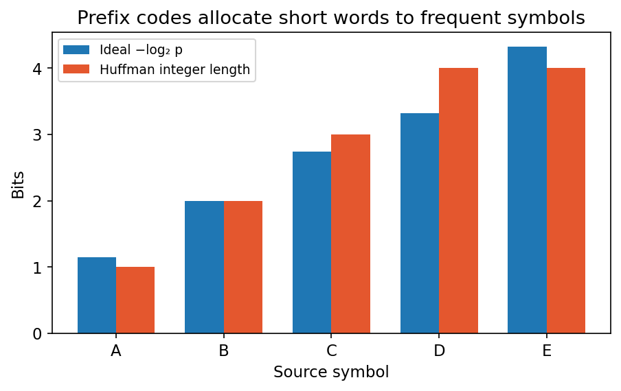
For probabilities 0.45, 0.25, 0.15, 0.10 and 0.05, the merge sequence is easy to follow by hand. Combine 0.05 with 0.10 to form 0.15. Combine that temporary weight with the original 0.15 to form 0.30. Then combine 0.25 with 0.30 to form 0.55, and finally 0.45 with 0.55 to form one.
A symbol’s code length is the number of merges between its leaf and the root. The resulting lengths are 1, 2, 3, 4 and 4. One valid assignment is:
| Symbol | Probability | Codeword | Length |
|---|---|---|---|
| A | 0.45 | 0 | 1 |
| B | 0.25 | 10 | 2 |
| C | 0.15 | 110 | 3 |
| D | 0.10 | 1110 | 4 |
| E | 0.05 | 1111 | 4 |
The code is prefix-free: after reading 0, the receiver immediately knows A; after reading 111, it still needs one more bit to decide between D and E. Left–right swaps can change codewords while preserving their lengths and expected cost.
The Kraft sum is . Expected length is bits per symbol. Source entropy is approximately 1.977235 bits, so this symbol code pays about 0.022765 bits of rounding mismatch per symbol. A fixed three-bit code would be sufficient for five symbols, but would spend an extra bit on every symbol relative to this expected length.
Notice that A’s one-bit description is shorter than its ideal surprise . Other symbols compensate. The theorem constrains the probability-weighted average, rather than requiring every individual codeword to be at least its own surprise. The program below may choose different bit labels for tied nodes, but reproduces these lengths and the two-bit expectation.
Code: build a tree, encode, decode and account for length
This complete example uses the same synthetic probabilities as the figure. It tests every pair of codewords for prefix freedom and reconstructs an independently sampled message. The printed payload excludes a transmitted tree and length header; those exclusions are explicit.
Code · Python · 42 lines
import heapq
import itertools
import numpy as np

symbols = list("ABCDE")
p = np.array([0.45, 0.25, 0.15, 0.10, 0.05])
counter = itertools.count()
heap = [(float(w), next(counter), s) for s, w in zip(symbols, p)]
heapq.heapify(heap)
while len(heap) > 1:
    wa, _, a = heapq.heappop(heap)
    wb, _, b = heapq.heappop(heap)
    heapq.heappush(heap, (wa + wb, next(counter), (a, b)))
tree = heap[0][2]
code = {}
def visit(node, prefix=""):
    if isinstance(node, str):
        code[node] = prefix or "0"
    else:
        visit(node[0], prefix + "0")
        visit(node[1], prefix + "1")
visit(tree)
assert all(not b.startswith(a) for i, a in enumerate(code.values())
           for j, b in enumerate(code.values()) if i != j)

rng = np.random.default_rng(34)
message = "".join(rng.choice(symbols, size=2000, p=p))
payload = "".join(code[s] for s in message)
inverse = {v: k for k, v in code.items()}
decoded, prefix = [], ""
for bit in payload:
    prefix += bit
    if prefix in inverse:
        decoded.append(inverse[prefix])
        prefix = ""
assert not prefix and "".join(decoded) == message
entropy = -np.sum(p * np.log2(p))
expected = sum(w * len(code[s]) for s, w in zip(symbols, p))
assert entropy <= expected < entropy + 1
print("Code:", code)
print("Entropy / expected length:", entropy, expected)
print("Payload bits per symbol:", len(payload) / len(message))
The entropy bound concerns expected length under the source, not every individual finite message. A particular sample can be shorter or longer than the expected rate. Tree transmission may dominate a tiny message; sharing a stable alphabet model across many messages amortizes it.
If probabilities are estimated from the message itself, the receiver cannot use that estimate unless it is transmitted or reproducible from already decoded symbols. Fitting a histogram and reporting only the resulting payload hides a real model cost.
Arithmetic coding: identify an interval for the whole message
Start with a unit interval. Each observed symbol selects a probability-sized subinterval. Repeated selection leaves a small interval that uniquely describes the whole message.
With cumulative model probability below symbol and conditional probability , update bounds by
Here is the interval after symbols, is the current symbol, and use the same already decoded history at both endpoints, and the initial interval is . The second update uses the old lower bound, not the newly updated one.
The final width is
Here is message length and the model’s joint probability. A sufficiently short binary description selecting a point or contained dyadic interval identifies the message. Ideal interval schemes incur only a bounded termination overhead for the whole block, rather than integer rounding at every symbol.
Practical implementations use finite integer registers, renormalization and explicit termination. A real number is not a transmitted object, and infinitely precise arithmetic is not a production codec. The short example below deliberately uses exact rational values to demonstrate the interval invariant without pretending to implement a full file format.
Read the first three interval updates
Use the example’s ordered model: A has probability , B has , and C has . Their cumulative starts are 0, and . For the prefix ABA, the updates are:
| Symbols read | Lower bound | Upper bound | Width |
|---|---|---|---|
| none | 0 | 1 | 1 |
A | 0 | ||
AB | |||
ABA |
After A, the available interval has width . B selects the portion from one half to five sixths within that interval, giving lower bound and upper bound . The next A takes the lower half of this width- interval. The final width is , exactly the model probability of ABA.
To decode, normalize the tag’s position inside the current interval. That normalized position selects A, B or C using the same cumulative partition. The receiver then updates the interval and repeats. The model and message length make the process reversible; the tiny interval explains the ideal description cost. Exact rational tags teach the mechanism, while finite integer implementations decide which actual bits to emit.
Code: a short exact interval round trip
The encoder outputs a rational tag, while the decoder is supplied the shared model and message length. The numerator and denominator are conceptual side information here; their serialized size is not claimed to be the optimal arithmetic-code length.
Code · Python · 34 lines
from fractions import Fraction

model = {"A": Fraction(1, 2), "B": Fraction(1, 3), "C": Fraction(1, 6)}
message = "ABACAB"
cumulative = {}
running = Fraction(0)
for symbol, probability in model.items():
    cumulative[symbol] = running
    running += probability
assert running == 1
low, high = Fraction(0), Fraction(1)
joint = Fraction(1)
for symbol in message:
    width = high - low
    old_low = low
    low = old_low + width * cumulative[symbol]
    high = old_low + width * (cumulative[symbol] + model[symbol])
    joint *= model[symbol]
assert high - low == joint
tag = (low + high) / 2

low_d, high_d = Fraction(0), Fraction(1)
decoded = []
for _ in range(len(message)):
    position = (tag - low_d) / (high_d - low_d)
    symbol = next(s for s in model
                  if cumulative[s] <= position < cumulative[s] + model[s])
    width, old_low = high_d - low_d, low_d
    low_d = old_low + width * cumulative[symbol]
    high_d = old_low + width * (cumulative[symbol] + model[symbol])
    decoded.append(symbol)
assert "".join(decoded) == message
print("Final interval:", low, high, "width:", high - low)
print("Exact decoded message:", "".join(decoded))
A zero model probability for a real symbol makes the interval vanish. The codec needs a positive escape route or an alphabet model covering all valid inputs. Merely clipping probabilities in the encoder is insufficient unless the decoder applies the same normalization and integer quantization.
Modeling cost is cross-entropy, not just entropy
An excellent bit-packing algorithm cannot repair a poor probability model. Unexpected symbols still need long descriptions.
For actual block distribution and coding model ,
Here averages under the actual source, is actual block entropy, and the divergence compares full block distributions. Finite coder and framing overhead adds further bits.
A model that uses preceding symbols can approach an entropy rate rather than just marginal entropy. An independence model on a persistent Markov sequence throws away predictable repetition. Conversely, a richer context model can overfit, require excessive memory, or assign fragile probabilities to unseen histories.
For evaluation, reserve independent recordings or acquisition groups. Report actual serialized size, including headers, model selection flags and required side streams. If weights are pretrained and permanently shared, state that convention; if weights are adapted per message, count their updates.
The relevant comparison is a complete encoder–decoder protocol under common assumptions. Comparing an ideal log-probability from one method with actual bytes from another can be useful diagnostically, but it is not a direct codec comparison.
Framing and malformed streams
An honest experiment also specifies what happens at the boundary of a message. A prefix tree tells the decoder where a symbol ends; it does not necessarily tell the decoder when the entire stream ends. A length header, end-of-message symbol or container boundary provides that separate fact.
Padding to a byte boundary can add bits that look like valid codewords. The receiver therefore needs the number of meaningful bits or the original symbol count. In the tree example, the payload is a Python string of bits used for teaching, not a byte-efficient container.
The decoder should reject an incomplete final codeword and impossible transitions instead of silently returning a shorter result. A checksum or other integrity mechanism may detect corruption, but detecting a damaged file is a separate requirement from compressing an undamaged one. If such a mechanism is part of the chosen protocol, its transmitted size also counts.
These details matter most for small messages and fair comparisons. Asymptotic statements can make a fixed header negligible per symbol, while an actual short file still pays every header bit.
Universal coding learns while decoding
When the source probability is unknown, both endpoints can update the same predictor from symbols already transmitted. No future symbol needs to be revealed for that update.
A sequential model factors as
Here is the preceding decoded history, and is a normalized conditional distribution. The encoder observes the current symbol; the decoder learns it from the interval and then performs the same state update.
For an unknown independent Bernoulli source, the Krichevsky–Trofimov predictor uses
Here counts previous ones and is the number of previous observations. The denominator is previous count plus one. Half-count smoothing gives positive probability to either next symbol, including the first observation [1].
This predictor is the posterior predictive distribution of a Bernoulli mixture with a beta half-count prior. It is universal for the stated Bernoulli family in the appropriate asymptotic coding sense; it is not automatically universal for arbitrary dependent sources.
Define sequence regret against an oracle model:
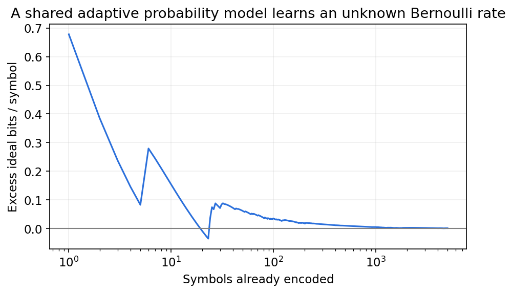
Here is the chosen oracle source and the adaptive model. Expected regret under that fixed source is a block divergence and nonnegative. Realized regret on one sample may be negative, because the mixture can assign that particular sample higher probability than the oracle.
Code: adaptation and an abrupt source change
This complete experiment measures ideal sequential lengths. It compares a fixed fair-bit model, a matched oracle and half-count adaptation. A second sequence changes its generating probability halfway through, illustrating the limitation of a stationary count model.
Code · Python · 22 lines
import numpy as np

rng = np.random.default_rng(23)
def adaptive_length(bits):
    ones, loss = 0, 0.0
    for t, bit in enumerate(bits):
        q = (ones + 0.5) / (t + 1)
        loss -= np.log2(q if bit else 1 - q)
        ones += int(bit)
    return loss

for n in [100, 1000, 5000]:
    bits = rng.binomial(1, 0.2, size=n)
    oracle = -np.sum(bits * np.log2(0.2) + (1 - bits) * np.log2(0.8))
    print("Length:", n, "oracle:", oracle / n,
          "adaptive:", adaptive_length(bits) / n, "fair model:", 1.0)
bits = np.r_[rng.binomial(1, 0.1, size=2500),
             rng.binomial(1, 0.9, size=2500)]
one_model = adaptive_length(bits)
two_models = adaptive_length(bits[:2500]) + adaptive_length(bits[2500:])
print("Changed source, whole / reset ideal rate:", one_model / 5000, two_models / 5000)
assert two_models < one_model
The reset comparison supplies the change point for free. A real codec must identify it or apply a predetermined reset schedule shared with the receiver. Counting a reset’s benefit while omitting its signaling cost overstates the achievable saving.
There are two different benchmarks: regret against a fixed oracle probability, and regret against the best parameter fitted retrospectively to the observed sequence. They are not interchangeable. A finite sample may favor a parameter different from its generating probability, even when the source is correctly specified.
See a causal predictor learn one symbol at a time
Before any observation, the half-count model assigns either bit probability . If the decoded prefix is 001, the next-one probability is , while next-zero probability is . Both endpoints obtain this state from the same prefix, so neither needs a transmitted histogram.
The model pays uncertainty early because it does not know the source bias. As counts accumulate under a fixed Bernoulli source, that initial learning cost is spread across more symbols. An alternating string has fair overall counts but perfect predictability from its previous symbol. The count-only model misses that relationship and keeps predicting near one half. Universal within a Bernoulli family therefore means learning an unknown bias, not learning every possible sequence structure.
Dictionaries, dependence and universal source classes
A dictionary coder learns recurring phrases rather than only symbol frequencies. Long repeated patterns can then be represented by references to earlier phrases.
Lempel–Ziv families construct descriptions from a growing set of previously observed strings [1]. Their asymptotic universality results specify a source class, such as stationary ergodic finite-alphabet processes, and a precise algorithm. They do not assert that any dictionary implementation beats every probabilistic model on every finite file.
Dictionary entries, phrase boundaries and reference indices must be reproducible by the decoder. As the dictionary grows, indices need more bits. A dictionary parser’s phrase count is not itself the compressed length; an integer coding rule and termination format are also needed.
Different source structures favor different mechanisms. A single-symbol predictor captures a bias; a context predictor captures short dependencies; phrase dictionaries exploit repeated substrings; a learned model may exploit structure shared across a training population. All still require reversible symbol transmission for a lossless claim.
Universality is relative to a benchmark and limiting regime. Unknown stationarity parameters are one problem; a changing alphabet or arbitrary adversarial source is another. Memory constraints, latency, short messages and reset policy can dominate the asymptotic benefit.
It is useful to ask four questions before quoting a universal-rate result: what class of sources is covered; what reference length is used; whether convergence is in expectation or along realizations; and whether model, dictionary and framing costs are included.
Kolmogorov complexity is an ideal limit of description
Imagine the shortest computer program that prints a string and stops. Structured strings can have short programs; most long strings cannot.
Relative to a fixed universal description machine , define
Here is a finite string, a terminating program for machine , and its program length in bits. Some formulations use prefix-free programs; the machine and convention must be stated [1].
Changing between suitable universal machines alters complexity by an additive machine-dependent constant. That does not make the value practically machine-independent for short strings. More importantly, the exact shortest-program function is not computable in general. One cannot turn the definition into an algorithm that always finds the best compressor.
A lossless compressor gives an upper bound on description complexity once its decoder and framing are included. Its output length is not the exact Kolmogorov complexity. Nor does a compressor failing to shorten a string prove the string is algorithmically random.
A counting argument shows why no injective compressor can shorten every fixed-length input. There are more length- strings than binary descriptions shorter than . Any scheme giving some inputs shorter descriptions must leave other inputs unshortened or longer, under an honest boundary convention.
This is compatible with excellent compression on a structured source distribution. Compression exploits nonuniform probability or repeated structure; it does not remove the counting constraint across all possible inputs.
Modern view
Yang, Mandt and Theis’s published 2023 monograph [4] separates lossless probability coding from lossy representation design. Its lossless taxonomy includes autoregressive, latent-variable and invertible models; its discussion emphasizes compatibility between model factorization and the entropy coder. We use that taxonomy to ask how probabilities reach an executable decoder.
A modern autoregressive network can replace the simple count predictor while retaining the chain-rule protocol. Its next-symbol probabilities must be available from the already decoded context. Latent-variable models need a specific protocol for any transmitted latent information; a low variational training objective is not automatically the final bitstream length.
The 2026 proposed learning chapter by El Gamal [5] provides a current divergence-centered connection between compression and statistical learning. It is a draft chapter. The classical mismatch identity remains useful: improved predictive probability can reduce ideal coding cost, while computation and synchronization determine whether that reduction is practical.
Open problems include adapting efficiently to distribution shifts, reducing sequential decoding cost, comparing complete formats fairly, and making model updates affordable for small messages. A larger predictor can save payload bits and simultaneously consume more shared memory or computation.
For a concrete evaluation, record three quantities separately: held-out negative log-probability, actual file size including required side information, and encoder/decoder runtime under the same hardware assumptions. Only the second establishes an achieved compression ratio; only a round-trip assertion establishes exact reconstruction.
The next chapter switches roles: a source coder removes predictable redundancy, while a channel coder introduces carefully structured redundancy to survive noise. Both use probability, but they solve different reconstruction problems.
Key takeaways
- Losslessness is an exact encoder–decoder identity with explicit boundaries.
- Kraft–McMillan constrains lengths; entropy lower-bounds their expected value.
- Huffman is optimal for the specified binary symbol-prefix problem.
- Arithmetic intervals spread rounding overhead across a whole message.
- Model mismatch adds divergence before finite implementation overhead.
- Adaptive coding requires synchronized causal updates and positive support.
- Universal performance depends on a stated source class and benchmark.
- Computable compression lengths are upper bounds on ideal algorithmic descriptions.
Exercises
- Construct two different symbol sequences that collide under codewords 0, 1 and 01. Explain why a supplied number of symbols may still leave ambiguity for other choices.
Hint
Start with the third symbol versus the first two.
- Verify the Kraft sum for lengths 1, 2, 3, 4, 4. Find a prefix tree realizing them and compare expected length under the example distribution.
Hint
Sum powers of two and assign leaves without ancestors.
- Change the Huffman probabilities to a uniform five-symbol source. Explain why ties change the tree but not the optimum expected length.
Hint
Keep a deterministic tie rule.
- Modify the exact arithmetic example to use a context-dependent binary predictor. Make the decoder update from decoded symbols and verify the final interval width.
Hint
Use exact half-count fractions and identical histories.
- Compare half-count adaptation on constant, alternating and independent biased binary strings. Identify which source structures a single count model misses.
Hint
Frequencies do not encode ordering.
- A learned predictor saves 0.1 ideal bits per symbol but requires 8,000 transmitted adaptation bits. Ignoring other changes, calculate the message length needed to offset that overhead.
Hint
Divide total overhead by the per-symbol saving.
References
- T. M. Cover and J. A. Thomas, Elements of Information Theory, 2nd ed., Wiley, 2006, Chapters 5, 13–14. Publisher book and contents.
- T. Weissman, “Variable Length Lossless Compression,” Stanford EE276 Lecture 4 notes, 2024. Primary lecture notes.
- T. Weissman, “Kraft-McMillan Inequality and Huffman Coding,” Stanford EE276 Lecture 5 notes, 2024. Primary lecture notes.
- Y. Yang, S. Mandt and L. Theis, “An Introduction to Neural Data Compression,” Foundations and Trends in Computer Graphics and Vision, 15(2), 113–200, 2023. Published monograph, author version.
- A. El Gamal, “Information Theory and Statistical Learning,” proposed textbook chapter, arXiv preprint, 2026. Draft and publication status.
Check your understanding
This tutorial has 6 exercises. Can you solve them without opening the hints?
Go to the exercises ↑Next IT 04 · Channel Capacity and Reliable Communication · 18 min