IT 06 · Rate–Distortion and Lossy Representations
Needs: IT 05 · Differential Entropy and Gaussian Channels
Navigate: this page and this track: Navigate: this page and this track
On this page
- What you’ll learn1 min
- The big picture1 min
- Choose the distortion before the codec1 min
- Operational and informational rate–distortion1 min
- Basic shape and zero-rate reconstruction1 min
- Binary sources with Hamming error2 min
- A Gaussian source under squared error1 min
- Why covering differs from channel packing1 min
- Compute a finite test channel2 min
- Scalar quantization is a concrete achievable design1 min
- Parallel Gaussian sources use reverse water-filling2 min
- Comparing operating points without changing the problem1 min
- Representations, tasks and learned rate penalties1 min
- Modern view1 min
- Key takeaways1 min
- Exercises1 min
- References
Information Theory
Explore this chapter 1 interactive experiment
Inspect the Bernoulli rate–distortion curve and an attaining joint distribution under Hamming error.
What you’ll learn
- Specify a distortion function before calling a reconstruction acceptable.
- Distinguish operational rate from an informational test channel.
- Derive Bernoulli/Hamming and Gaussian/squared-error rate–distortion functions.
- Explain covering achievability and the converse’s information accounting.
- Compute finite-alphabet rate–distortion points with alternating updates.
- Relate practical quantization and learned objectives to honest rate and quality measurements.
The big picture
Lossless coding asks for the exact original. Lossy coding asks for a useful substitute. The second question cannot be answered until “useful” has a mathematical meaning: which differences matter, how much they cost, and whether the constraint concerns average error or rare large failures.
This chapter follows Cover and Thomas’s Chapter 10 [1] and Stanford’s primary rate–distortion notes [2,3]. The central result minimizes mutual information over hypothetical reconstruction laws. That optimization defines a limit; it does not by itself build a finite file format or guarantee the behavior of a neural decoder.
The distinction connects directly to vision. A pixel reconstruction, a machine-readable feature and a plausible generated image preserve different properties. Their rates and distortions should be compared only after the objectives and resource conventions are made explicit.
Choose the distortion before the codec
An error measure specifies which source differences the receiver tolerates. There is no universal distortion score that captures every task.
Let be a source symbol and a reconstruction in a possibly different alphabet. A nonnegative distortion function is . For a length- block,
Here indexes symbols, is block length, and is average per-symbol distortion. A common constraint is , with the allowed average and expectation under the specified source and code.
Hamming distortion is zero for a correct symbol and one otherwise. Squared-error distortion is for real amplitudes. They answer different questions: the first counts mismatches; the second weights large numerical deviations more heavily.
Squared error also depends on units. Scaling source and reconstruction by multiplies distortion by . A rate–distortion curve should therefore state source normalization, dimensional averaging and the distortion’s units.
The usual additive model assigns a cost to each symbol and averages. A structured task may need a block-level criterion: preserving a relation, a rare feature or a decision. It can still be studied, but it is not automatically the same single-letter problem.
Average distortion does not bound the worst individual reconstruction. A small mean can coexist with rare large errors. If the application requires a tail probability, a maximum error or per-group guarantees, include that separate condition rather than reading it into a mean.
The reproduction alphabet is another part of the definition. Restricting reconstructions to a small codebook, integer pixels or a particular model family reduces the feasible set. An unconstrained theoretical optimum may then be unattainable for that design. Conversely, allowing a receiver to output a task label rather than an image changes both the alphabet and the distortion question. A fair comparison should state these choices before showing any rates, so readers can tell whether two systems preserve the same object.
Operational and informational rate–distortion
A real code sends one of finitely many descriptions. A test channel describes a possible statistical relationship between source and reconstruction. The theorem connects their asymptotic limits.
A block encoder maps to one of indices, and a decoder maps the index to . Its fixed rate is
Here is the number of possible transmitted descriptions and is bits per source symbol. The operational function is the infimum of asymptotically achievable rates at the specified distortion.
For an independent memoryless source and an appropriate additive distortion setting, the rate–distortion theorem gives
Here the source law is fixed, while varies over normalized reconstruction laws. The minimum notation applies to settings where a minimizer exists; broader continuous cases can require an infimum and regularity conditions [1,2].
This reconstruction law is often called a test channel. Unlike communication capacity, its input source is not optimized. Capacity maximizes transmitted information under a given physical channel; rate–distortion minimizes required information under a reconstruction constraint.
A stochastic test channel is a mathematical object describing the desired joint distribution. The operational theorem uses block codes to approach its information rate. Independently drawing a noisy reconstruction for every source symbol does not itself explain how few bits a receiver needs to reproduce those draws.
Basic shape and zero-rate reconstruction
Allowing more error cannot require more bits. At some distortion, the receiver can always output one fixed reconstruction and need no message.
Define
Here is the best constant-reconstruction average distortion and is chosen independently of the observed source. At , zero rate is feasible.
The function is nonnegative, nonincreasing and convex in the standard setting. Nonincrease follows because a larger distortion allowance includes all previously feasible codes.
Convexity has a time-sharing interpretation. For fraction of a long block, use one code; for the rest, use another. Then
Here is the share, the component distortions, and the right side their average rates. Predetermined block boundaries avoid per-symbol signaling of the choice.
At zero distortion, a finite source with an identity-only zero-cost condition returns the ordinary entropy limit. If the distortion considers several different source values equally correct, zero distortion may require less than source entropy. For a genuinely continuous Gaussian source under squared error, the zero-distortion rate diverges.
Those qualifications matter. Saying “zero distortion means entropy” without specifying the distortion’s zero set or alphabet can erase the very reason that a task representation compresses.
Binary sources with Hamming error
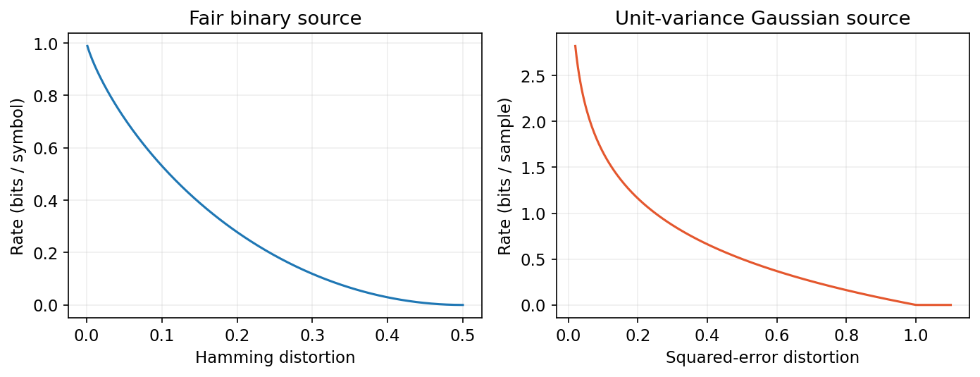
A fair binary source costs one bit per symbol to preserve exactly. Permitting a controlled mismatch fraction reduces the necessary rate.
For with and Hamming distortion,
Here is the probability of one, is mismatch probability, and is binary entropy. The zero-rate reconstruction is always zero, which makes errors on fraction of source symbols.
To obtain a lower bound, let be the mismatch indicator, where denotes binary exclusive-or. Then
Here has probability of one at most , and binary entropy increases over that range. Conditioning cannot increase discrete entropy.
Equality is reached by a backward construction: choose and independent , then set . The reconstruction probability satisfies
Here avoids the singular fair-source endpoint; endpoints follow by continuity or a direct constant reconstruction. The construction gives the required source law and makes mismatch independent of reconstruction.
For a fair source, the curve reduces to through . For a biased source, naively flipping forward with probability generally does not attain the same optimum. The direction of the independence condition is part of the derivation.
Build the optimal binary joint table
The backward construction becomes clearer when its probabilities are written out. Take source probability and allowed mismatch . If , independence of reconstruction and mismatch gives
Here is the required source-one probability, the reconstruction-one probability and the independent backward flip probability. Solving gives . Multiplying reconstruction probabilities by independent error probabilities yields:
| Joint probability | Source marginal | ||
|---|---|---|---|
| 0.7875 | 0.0125 | 0.8 | |
| 0.0875 | 0.1125 | 0.2 | |
| Reconstruction marginal | 0.875 | 0.125 | 1.0 |
The off-diagonal entries sum to 0.1, exactly the allowed distortion. Dividing either reconstruction column by its total shows a 0.1 probability that the source differs from that reconstruction. Thus and required information is bits per source symbol.
The equivalent forward conditional channel is asymmetric. Given , it outputs one with probability . Given , it outputs zero with probability . The large error on rare ones and small error on common zeros achieve the specified overall error while meeting the optimal posterior uncertainty.
By contrast, independently flipping the source forward with probability 0.1 preserves the same average distortion, but produces reconstruction-one probability 0.26. Its information is bits, greater than the optimum. “Ten percent noise” is therefore insufficient to identify an optimal test channel: the direction and independence relationship matter.
Code · Python · 20 lines
import numpy as np

def entropy(p):
    p = np.asarray(p, dtype=float)
    positive = p > 0
    return -np.sum(p[positive] * np.log2(p[positive]))

source_one, D = 0.2, 0.1
q = (source_one-D)/(1-2*D)
joint = np.array([[(1-q)*(1-D), q*D],
                  [(1-q)*D, q*(1-D)]])
px, pr = joint.sum(axis=1), joint.sum(axis=0)
information = entropy(px)+entropy(pr)-entropy(joint)
assert np.allclose(px, [0.8, 0.2])
assert np.isclose(joint[0, 1]+joint[1, 0], D)
assert np.allclose([joint[1, 0]/pr[0], joint[0, 1]/pr[1]], D)
exact = entropy(px)-entropy([D, 1-D])
assert np.isclose(information, exact)
print("Backward joint table:", joint)
print("Optimal information:", information)
This calculation verifies a statistical optimum. It still needs a long-block code to translate that information rate into a transmitted reconstruction index.
A Gaussian source under squared error
A broad Gaussian source needs more bits for the same absolute precision. Requiring smaller error grows rate logarithmically.
For and ,
Here is source variance and the mean squared error in the same squared units. At , a zero reconstruction requires no bits. As , rate grows without bound [1,3].
Let be reconstruction error. For compatible finite differential entropies,
Here conditioning reduces differential entropy when mutual information is well defined, and Gaussian maximum entropy bounds error entropy by its second moment. The expression is a lower bound in the nonzero-rate range.
Achievability of the informational minimum uses independent and , with . This is again a backward test channel; the error is independent of reconstruction, not of the source.
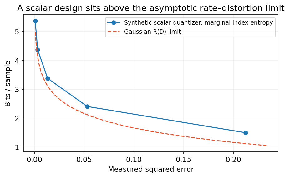
The equivalent distortion–rate relation is . It refers to asymptotically optimized block coding. A simple scalar quantizer generally lies above the limit at its resulting rate.
Code: test the Gaussian backward construction
This complete synthetic experiment verifies the source variance, error variance and information formula. It does not serialize a block code; it tests the optimizing joint distribution.
Code · Python · 16 lines
import numpy as np

rng = np.random.default_rng(38)
variance, distortion = 1.0, 0.2
reconstruction = rng.normal(0, np.sqrt(variance-distortion), size=100000)
error = rng.normal(0, np.sqrt(distortion), size=100000)
source = reconstruction + error
rho = np.corrcoef(source, reconstruction)[0, 1]
information = -0.5 * np.log2(1-rho**2)
exact = 0.5 * np.log2(variance/distortion)
print("Source variance / error MSE:", source.var(), np.mean(error**2))
print("Error-reconstruction correlation:", np.corrcoef(error, reconstruction)[0, 1])
print("Gaussian-model information / exact rate:", information, exact)
assert abs(source.var()-variance) < 0.02
assert abs(np.mean(error**2)-distortion) < 0.01
assert abs(information-exact) < 0.02
Independence is built into the sampling, while the finite correlation is only a check. Small empirical correlation alone would not establish independence for arbitrary non-Gaussian variables.
Why covering differs from channel packing
A lossy source code needs enough reconstruction representatives to cover likely source blocks within acceptable error. A channel code instead separates transmitted representatives to resist noise.
Fix a feasible source–reconstruction joint distribution. Draw many reconstruction codewords from its marginal. For a typical source block, a random reconstruction has a matching joint relationship with a probability on the exponential scale .
With more than approximately representatives and a small rate margin, a suitable match becomes likely. The encoder selects its index; the decoder returns that shared reconstruction. Joint typicality connects the chosen pair to the target distortion.
This is a covering argument. The exact proof needs typicality definitions and source/distortion assumptions; the exponential scale explains the rate without serving as a finite-code performance formula.
The converse uses the transmitted index :
Here ranges over descriptions, , , and the source is memoryless. The first information bound uses that reconstruction is determined by the index; the per-symbol step uses source independence and the informational definition; the last step is convexity.
The code cannot convey more information about the source than its index contains. This accounting explains why a decoder’s sophisticated prior cannot recover arbitrary missing details at no source rate. It can choose useful or probable reconstructions according to the specified distortion.
Compute a finite test channel
For discrete alphabets, alternate between a reconstruction marginal and a source-conditioned reconstruction law. A penalty parameter moves along the rate–distortion frontier.
Minimize the natural-unit objective with . Given current reconstruction marginal ,
Here is the fixed source law, is the test channel, indexes reconstructions, and measures distortion penalty in natural units. Rates reported in bits divide the natural-unit information by .
The Blahut–Arimoto alternating computation is discussed in the textbook [1]. A positive initial marginal covers all candidate reconstruction symbols. At a solution, compute actual distortion and mutual information; do not label itself as the distortion.
Where the exponential test-channel update comes from
The alternating rule follows from a constrained minimization, not a heuristic resemblance to a probability distribution. Temporarily fix a positive reconstruction marginal . For source state , minimize the row contribution
Here is the conditional probability of reconstruction given source , the fixed reference marginal, distortion and the natural-unit distortion penalty. The positive source weight multiplies this row and does not change its minimizing conditional distribution.
Add a row-normalization multiplier and differentiate with respect to . The stationary equation is . Exponentiation makes proportional to ; row normalization supplies the denominator in the displayed update.
Next fix . Its induced marginal minimizes the cross-entropy part over normalized . Alternating these two steps lowers the penalized objective under the stated finite-alphabet setting. It also explains the geometry: larger concentrates each row toward low-distortion reconstructions, while the marginal factor favors reconstructions used by the population.
For a fair binary source with Hamming distortion, symmetry keeps uniform. Off-diagonal probability is therefore , and the rate is . This analytic relation is what the code checks. It gives a direct interpretation of the penalty without mistaking the penalty value for an achieved distortion.
Code: compare with exact binary curves
The implementation checks convergence of the reconstruction marginal and validates the resulting points against independent analytic formulas. Its tolerance is a numerical update tolerance, not the upper–lower capacity gap from the previous chapter.
Code · Python · 37 lines
import numpy as np
from scipy.special import logsumexp

def entropy(p):
    p = np.asarray(p)
    return -np.sum(p[p > 0] * np.log2(p[p > 0]))
def rd_point(p, distortion_matrix, beta):
    p = np.asarray(p, dtype=float)
    d = np.asarray(distortion_matrix, dtype=float)
    q = np.full(d.shape[1], 1/d.shape[1])
    for _ in range(50000):
        scores = np.log(q)[None, :] - beta*d
        V = np.exp(scores-logsumexp(scores, axis=1, keepdims=True))
        updated = p @ V
        if np.max(abs(updated-q)) < 1e-13:
            q = updated
            break
        q = updated
    else:
        raise RuntimeError("Rate-distortion updates did not converge")
    joint = p[:, None]*V
    positive = joint > 0
    ratio = np.divide(V, q[None, :], out=np.ones_like(V), where=positive)
    rate = np.sum(joint[positive]*np.log2(ratio[positive]))
    distortion = np.sum(joint*d)
    return rate, distortion, V

d = np.array([[0, 1], [1, 0]])
for beta in [0.0, 1.0, 2.0, 4.0]:
    rate, D, V = rd_point([0.5, 0.5], d, beta)
    exact = 1-entropy([D, 1-D])
    assert abs(rate-exact) < 1e-10
    print("Penalty / D / rate / exact:", beta, D, rate, exact)
rate, D, V = rd_point([0.8, 0.2], d, 4.0)
exact = entropy([0.8, 0.2])-entropy([D, 1-D])
assert D < 0.2 and abs(rate-exact) < 1e-9
print("Biased-source D / rate / exact:", D, rate, exact)
For arbitrary distortion matrices, a small marginal-update difference is a useful convergence check but not a rigorous global numerical certificate. Inspect objective changes, supports and independent special cases. Very large penalties can underflow probability entries or require a more careful implementation.
Scalar quantization is a concrete achievable design
Round source values to a finite-resolution grid, then losslessly describe their grid indices. The rounding creates distortion; probability coding reduces index rate.
With step , use
Here is the discrete index, the grid reconstruction, and its squared-error distortion. An entropy-coded index has a rate governed by the index distribution, plus practical coding costs.
For sufficiently smooth densities at small step, a common approximation is . The approximation treats quantization error as approximately uniform inside a cell; it need not hold at coarse steps, near clipping or for structured concentrated values.
Code · Python · 14 lines
import numpy as np

rng = np.random.default_rng(26)
source = rng.normal(size=20000)
for step in [0.1, 0.2, 0.4, 0.8, 1.6]:
    index = np.rint(source/step).astype(int)
    reconstruction = step*index
    _, counts = np.unique(index, return_counts=True)
    p = counts/counts.sum()
    rate_estimate = -np.sum(p*np.log2(p))
    mse = np.mean((source-reconstruction)**2)
    gaussian_limit = max(0, 0.5*np.log2(1/mse))
    print("Step / index entropy / MSE / reference rate:",
          step, rate_estimate, mse, gaussian_limit)
The empirical distribution is measured on the same sample being quantized, so it is a descriptive statistic. To compare a learned entropy model, fit it on separate training observations and score a fixed held-out set. Transmit or share its parameters under an explicit convention.
Index entropy is not an actual compressed file size. A codec also specifies index support, out-of-range handling, reconstruction step, message length and entropy-coder termination. Finite empirical estimates can fluctuate around theoretical relationships without invalidating the population theorem.
Parallel Gaussian sources use reverse water-filling
A limited description budget should preserve the most variable source directions more carefully. Low-variance directions can be discarded when their entire variation is within the error allowance.
For independent Gaussian source coordinates with variances , use total squared-error budget :
Here indexes coordinates, is their allocated mean squared error, and is bits per complete source vector. Within the positive-rate range, differentiating the objective makes the optimal active distortions equal:
Here is the reverse water level, chosen for a budget below total source variance. A coordinate with variance below the level is reconstructed as its mean, paying its full variance and no rate.
The similarity to channel water-filling is instructive, but the roles differ. Channel allocation spends signal power above noise floors to maximize transported information. Source allocation permits error up to source variances to minimize required description information.
For a correlated Gaussian vector, an orthogonal covariance eigenbasis produces independent coordinates and preserves total squared error. The allocation then acts on eigenvalues. A nonlinear task distortion or a non-Gaussian distribution need not reduce to this same eigenvalue calculation.
This also explains the benefit and limitation of a low-dimensional reconstruction. Discarding a low-variance coordinate is inexpensive for total squared error, but that coordinate could still be decisive for a particular label. Task relevance and variance are different criteria.
A reverse-water-filling allocation
Take three independent Gaussian coordinates with variances 4, 1 and 0.25, and allow total squared error one per vector. Giving each coordinate error one third would waste the third coordinate’s budget: reconstructing it as zero already incurs only 0.25.
The optimal common error level for the remaining two coordinates solves , so . The distortions are 0.375, 0.375 and 0.25; their sum is one. Required rate is
Here is bits per three-coordinate source vector. The first two coordinates receive positive description rate, while the third is reconstructed as its mean and costs zero rate. The distortion budget is a sum per vector, not a mean per coordinate; dividing the budget by three would express the same operating point using a different convention.
The shared error level follows by differentiating each active coordinate’s rate: the magnitude of the rate decrease per extra unit of distortion is . Equalizing that marginal saving makes active equal. Once reaches its source variance, there is no further rate to save, so that coordinate leaves the active set.
A small-variance coordinate may still encode an important label. Reverse water-filling is optimal for this Gaussian squared-error problem, while a label-preservation requirement would need a different distortion. This example makes the link between optimization conditions and the actual receiver objective explicit.
Comparing operating points without changing the problem
A fair rate–distortion comparison keeps source data, quality criteria and resource assumptions fixed. Otherwise a better-looking curve may be solving an easier problem.
An empirical operating point consists of measured rate and measured distortion under one complete protocol. Its description should specify whether the rate is fixed length, average variable length, ideal negative log-probability or actual serialized bits.
The theoretical curve in this chapter uses a memoryless population source and asymptotically long codes. A finite experiment has sampling uncertainty, finite blocks, a restricted model family and implementation costs. Reporting all of those as one gap obscures which component is responsible.
Keep the same held-out observations for different codec settings. Fit quantizers, probability models and any learned transforms using training data. Use validation data to choose penalties or operating points. Reserve the final test set to estimate the selected protocol’s performance.
Report distortion across meaningful groups when the population is heterogeneous. An average over common cases can hide a subgroup whose reconstructions are much worse. This does not invalidate a mean-distortion theorem; it shows that the selected mean may not fully express the desired application.
Also state decoding randomness. A deterministic decoder and a randomized generative decoder can have different error distributions at the same stored index. Repeated reconstructions of the same test input reveal that variability; selecting the best random reconstruction after seeing the original introduces a selection step that a real receiver may not have.
Finally, keep shared side information comparable. A decoder with a task-specific database, pretrained prior or transmitted adaptation receives a different protocol from one without it. Shared resources can be useful, but their availability and cost convention need to accompany the claimed frontier.
Representations, tasks and learned rate penalties
A representation can discard irrelevant detail while preserving a task. That helps only when the retained task is specified and evaluated on the intended population.
A learned encoder may produce quantized latent with entropy model , while a decoder returns . A common training objective has the form
Here the first term is an ideal coding-cost surrogate in bits, balances the specified distortion, and expectations use the training distribution. This objective does not automatically equal the population rate–distortion function.
The latent alphabet, entropy-model mismatch, finite coder, side streams and model costs affect actual rate. The architecture restricts achievable reconstructions. Optimization can find a local or model-constrained tradeoff rather than the information-theoretic minimum.
If the receiver needs a label , an appropriate criterion can evaluate the decision inferred from instead of reconstructing all of . That is a different source-distortion problem. A feature preserving one label can discard information needed by a later, unrelated task.
A perceptual criterion may reward plausible texture even when texture differs from the source. A faithful reconstruction criterion may penalize the same change. Neither objective is universally correct; their distinction needs to remain visible in text, figures and evaluation.
Multiple distortions can be reported together without collapsing them into one unexplained score. For example, separate numerical fidelity, a stated task error and a distributional realism criterion.
Modern view
The 2023 monograph by Yang, Mandt and Theis [4] separates lossless entropy coding from lossy transform design, quantization, perceptual objectives and task-oriented coding. Its taxonomy helps locate which component of a learned system changes rate, which changes distortion, and which changes the evaluation goal.
Huang and Wu’s 2024 review [5] explicitly contrasts human and machine consumers of learned image compression. The shared lesson is that a compressed representation’s usefulness is receiver-dependent; one reconstruction score cannot establish preservation for every downstream analysis.
Hofer and Böhme’s 2024 preprint [6] develops a taxonomy of neural-image miscompression. It motivates examining the kinds of changed content, rather than assuming that average numerical error completely characterizes reconstruction behavior. We cite its verified preprint status.
Our inference from rate–distortion theory is to evaluate a frontier, not one favorable operating point: measured bitstream size versus explicitly defined distortion on a fixed test population. Keep source normalization, model-sharing assumptions and decoder resource budgets consistent.
Open questions include task transfer after irreversible compression, distortion measures for rare details, performance under distribution shift, and fair resource accounting for generative priors. Longer blocks or more elaborate decoders can improve a particular tradeoff while adding latency or relying on stronger shared assumptions.
The next chapter extends information beyond coding: divergence describes statistical evidence, maximum entropy selects distributions under constraints, and logarithmic growth connects prediction with decision-making.
Key takeaways
- Distortion defines what a lossy reconstruction is allowed to change.
- Rate–distortion fixes the source and optimizes a reconstruction law.
- Its standard frontier is nonincreasing and convex.
- Binary and Gaussian optima use carefully defined backward test channels.
- Covering and information accounting connect test channels to block codes.
- Alternating numerical updates require explicit logarithm and penalty units.
- Quantizer index entropy differs from actual serialized rate.
- Learned or perceptual objectives must be judged against their stated receiver and distortion.
Exercises
- For a Bernoulli source with probability 0.2, compute the zero-rate distortion and rates at distortions 0, 0.05 and 0.1.
Hint
Use within the nonzero-rate range.
- Construct the backward binary joint law at , . Compare it with independently flipping the source forward by 0.1.
Hint
Make mismatch independent of reconstruction.
- For a Gaussian source of variance 4, compute the rates needed for squared errors 1 and 0.25. Explain the result after changing coordinate units.
Hint
Rate depends on a variance-to-distortion ratio.
- Extend the finite test-channel code to a three-symbol source and an asymmetric distortion matrix. Report the penalty, actual rate and actual distortion separately.
Hint
Check row normalization and reconstruct the joint law.
- Add clipping to scalar quantization. Compare errors near the center and tails instead of reporting only the mean.
Hint
Track saturation cases separately.
- Design two different distortion functions for a tiny binary image: exact pixel preservation and preservation of whether any foreground pixel exists. Explain why their zero-distortion rates differ.
Hint
The task identifies equivalence classes of images.
References
- T. M. Cover and J. A. Thomas, Elements of Information Theory, 2nd ed., Wiley, 2006, Chapter 10. Publisher book and contents.
- T. Weissman, “Lossy Compression & Rate Distortion Theory,” Stanford EE276 Lecture 13 notes, 2024. Primary lecture notes.
- T. Weissman, “Lossy Compression & Rate Distortion Theory Continued,” Stanford EE276 Lecture 14 notes, 2024. Primary lecture notes.
- Y. Yang, S. Mandt and L. Theis, “An Introduction to Neural Data Compression,” Foundations and Trends in Computer Graphics and Vision, 15(2), 113–200, 2023. Published monograph, author version.
- C.-H. Huang and J.-L. Wu, “Unveiling the Future of Human and Machine Coding: A Survey of End-to-End Learned Image Compression,” Entropy, 26(5), 357, 2024. Published review.
- N. Hofer and R. Böhme, “A Taxonomy of Miscompressions: Preparing Image Forensics for Neural Compression,” arXiv preprint, 2024. Primary preprint.
Check your understanding
This tutorial has 6 exercises. Can you solve them without opening the hints?
Go to the exercises ↑Next IT 07 · Statistical Evidence, Maximum Entropy and Growth · 18 min