IT 07 · Statistical Evidence, Maximum Entropy and Growth
Needs: IT 06 · Rate–Distortion and Lossy Representations
Navigate: this page and this track: Navigate: this page and this track
On this page
- What you’ll learn1 min
- The big picture1 min
- Likelihood ratios compare explanations1 min
- Testing errors form a tradeoff3 min
- Empirical types reveal why divergence controls rare events2 min
- Asymmetric and symmetric hypothesis exponents1 min
- Sufficiency and data processing in inference1 min
- Fisher information measures local parameter sensitivity2 min
- Maximum entropy makes constraints explicit2 min
- Logarithmic growth turns mismatch into a decision cost1 min
- Universal mixtures connect portfolios with coding1 min
- Modern view1 min
- Key takeaways1 min
- Exercises1 min
- Supplementary notes
- References
Information Theory
Explore this chapter 1 interactive experiment
Slide a decision threshold across two exact binomial distributions and compute both error probabilities.
What you’ll learn
- Interpret a likelihood ratio as evidence rather than a posterior probability.
- Use empirical types to explain divergence-controlled rare-event rates.
- Distinguish hypothesis-testing error tradeoffs from parameter estimation.
- Derive Fisher information and a regular unbiased-estimation bound.
- Construct maximum-entropy distributions from explicit constraints.
- Relate log-optimal allocation and universal mixtures to coding regret.
The big picture
Information measures are not restricted to storage and communication. They also quantify how observations distinguish competing explanations, how strongly a distribution changes with a parameter, and how costly a poor predictive decision can become over repeated trials.
The book map is Cover and Thomas’s Chapter 11 for statistics, Chapter 12 for maximum entropy, Chapter 6 for gambling and coding, and Chapter 16 for portfolio theory [1]. Stanford’s method-of-types notes [2] provide an accessible primary finite-alphabet derivation.
We use mathematical decision games with fully specified probabilities and payoffs. Their purpose is to expose information identities, not to infer practical returns from historical data. In every section, distinguish the source law, the chosen model, the observed sample and the decision criterion.
Likelihood ratios compare explanations
A sample supports one model over another when that model assigns the sample a larger probability. Repeated independent observations add their log evidence.
For two fully specified distributions and with compatible support, define
Here is an observed length- sample, the final equality assumes independent observations under each model, and may be natural or base two if used consistently. Positive values favor in the likelihood comparison.
Under , expected base-two log ratio is . Under , it is . The different directions arise because expectation is taken under different laws.
A likelihood ratio is not a posterior probability. To calculate posterior odds, multiply by prior odds. To choose an action, incorporate the losses of wrong decisions. A threshold of zero is appropriate for certain symmetric prior-and-loss choices, not every test.
For simple hypotheses, the Neyman–Pearson likelihood-ratio principle describes the most powerful test at a specified false-alarm constraint [1]. “Simple” means the distributions are fixed, not families with unknown fitted parameters.
If parameters are estimated from the same sample, the test is a different procedure. Model selection, nuisance parameters and threshold calibration can alter its finite error behavior. It is useful to start with fully specified toy laws before interpreting a fitted classifier’s score as evidence.
Testing errors form a tradeoff
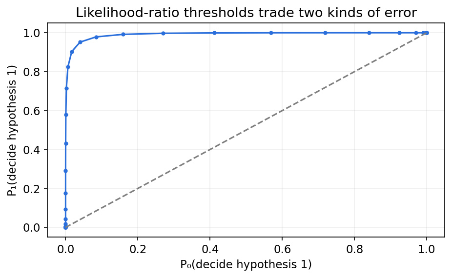
Making it harder to declare an alternative reduces false alarms but can miss more real alternatives. Neither error should disappear from the report.
Set null distribution and alternative . A rejection region gives
Here is the type-I error or false-alarm probability, the type-II error or missed-alternative probability, and the set where the test declares the alternative.
For Bernoulli probabilities , the log likelihood ratio of alternative to null is an increasing function of the count of ones. A threshold on that count therefore implements a likelihood-ratio test.
Discrete counts may prevent reaching an arbitrary false-alarm target exactly with a deterministic threshold. Randomization at a boundary can achieve an intermediate operating point mathematically; a deployed rule should state whether it uses such randomization.
Code: exact errors and a Monte Carlo check
This complete example chooses the first count threshold satisfying a 5% false-alarm limit and calculates its missed-alternative probability. It then verifies the two laws independently.
Code · Python · 17 lines
import numpy as np
from scipy.stats import binom

n, p0, p1 = 30, 0.3, 0.6
thresholds = np.arange(n+2)
false_alarm = binom.sf(thresholds-1, n, p0)
detection = binom.sf(thresholds-1, n, p1)
threshold = thresholds[np.flatnonzero(false_alarm <= 0.05)[0]]
alpha = binom.sf(threshold-1, n, p0)
beta = binom.cdf(threshold-1, n, p1)
rng = np.random.default_rng(40)
observed_alpha = np.mean(rng.binomial(n, p0, 100000) >= threshold)
observed_beta = np.mean(rng.binomial(n, p1, 100000) < threshold)
print("Threshold / alpha / beta:", threshold, alpha, beta)
print("Simulation alpha / beta:", observed_alpha, observed_beta)
assert abs(observed_alpha-alpha) < 0.005
assert abs(observed_beta-beta) < 0.005
The selected threshold uses known distributions, not a test-set search. In a learned application, tune the threshold on validation data and estimate its errors on separate test observations. Data groups or time dependence can change the effective independence assumption.
The proportion of alternatives in an evaluation set affects the frequency of correct declarations, but it does not change the two conditional errors for a fixed test and fixed laws. A test can have a small false-alarm probability and still produce many false declarations when alternatives are extremely rare. To interpret those declarations, combine the conditional errors with the intended prior prevalence. This is a direct consequence of conditional probability, not a failure of the likelihood-ratio principle. State whether a reported quantity is conditioned on the null, conditioned on the alternative, or conditioned on the test’s output.
Worked evidence is not the same as confidence
For the example’s null probability 0.3 and alternative probability 0.6, a length-30 block with ones has alternative-to-null log likelihood ratio
Here is the observed count, uses natural logarithms, and the two fractions compare the probabilities of one and zero under the competing laws. With 18 ones, , giving likelihood ratio about 317.748375. This evidence favors the alternative strongly.
If the prior alternative probability is 0.01, prior odds are . Posterior odds become approximately , corresponding to posterior probability about 0.762447. The likelihood ratio is not a 99.7% confidence value: the prior changes the posterior interpretation.
An even more practical distinction concerns all positive declarations from the threshold test. The code chooses threshold 14, with false-alarm probability about 0.040053 and missed-alternative probability about 0.048112. If only 1% of cases come from the alternative, the probability that a positive declaration is truly alternative is
Here is prior alternative prevalence, the test’s false-alarm probability and its missed-alternative probability. The notation denotes the event that the alternative generated the case. Most positives in this population are false alarms, even though each conditional error is below 5%.
This conclusion follows from counting expected positive cases from the two populations. It does not change the likelihood-ratio optimality result or the measured conditional errors. A decision report should name its conditioning event so readers can distinguish a particular sample’s posterior from the average composition of all positive declarations.
Code · Python · 14 lines
import numpy as np
from scipy.stats import binom

n, p0, p1, prior = 30, 0.3, 0.6, 0.01
count = 18
log_ratio = count*np.log(p1/p0)+(n-count)*np.log((1-p1)/(1-p0))
posterior = 1/(1+((1-prior)/prior)*np.exp(-log_ratio))
threshold = 14
alpha = binom.sf(threshold-1, n, p0)
beta = binom.cdf(threshold-1, n, p1)
positive_precision = prior*(1-beta)/(prior*(1-beta)+(1-prior)*alpha)
assert alpha <= 0.05 and binom.sf(threshold-2, n, p0) > 0.05
print("Likelihood ratio / sample posterior:", np.exp(log_ratio), posterior)
print("Probability alternative given positive:", positive_precision)
Empirical types reveal why divergence controls rare events
Many strings share the same histogram. Their number grows like an entropy exponent, while their individual source probabilities shrink like a cross-entropy exponent. The difference is divergence.
For a finite alphabet of size , the type of a length- sequence is its empirical symbol distribution. Its type class contains every sequence with those counts. Under independent source law ,
Here has type , is empirical entropy, and divergence is measured in bits. The formula follows by grouping identical log probabilities by count.
The class size is bounded, with a conservative polynomial factor, by
Here is the number of sequences; and are block length and alphabet size. Multiplying by one sequence probability gives
Here is total type-class probability. The polynomial factor matters at finite length but disappears from the normalized logarithmic exponent [1,2].
The orientation is worth emphasizing: the first argument is the unusual empirical type; the second is the source actually generating observations. This differs from a coding mismatch calculation averaged under a fixed true source.
For sets of empirical distributions, the dominant exponential behavior is governed by the smallest divergence among allowed types. Sanov’s theorem formalizes that large-deviation statement under its finite-alphabet and set-regularity conditions [1].
Code: exact binary type probability versus its exponent
This standalone example compares a binomial probability with the exponential bounds. It uses logarithms to avoid underflow and checks the finite polynomial gap.
Code · Python · 15 lines
import numpy as np
from scipy.stats import binom

q, target = 0.3, 0.6
for n in [30, 100, 300, 1000]:
    count = int(round(n*target))
    empirical = count/n
    divergence = (empirical*np.log2(empirical/q) +
                  (1-empirical)*np.log2((1-empirical)/(1-q)))
    negative_log_probability = -binom.logpmf(count, n, q)/np.log(2)
    exponent = n*divergence
    assert exponent <= negative_log_probability + 1e-10
    assert negative_log_probability <= exponent + 2*np.log2(n+1) + 1e-10
    print("Length / observed normalized exponent / divergence:",
          n, negative_log_probability/n, divergence)
A rare exact type is not the same event as a one-sided tail or a typical neighborhood. The exponent governing a tail comes from optimizing over all counts in that event, not blindly substituting its most extreme count.
From one type to a set of types
For an event defined by a collection of empirical distributions, there are at most possible types. Summing the individual upper bounds gives
Here is the subset of realizable at length , is a candidate type, and the infimum selects the least surprising type under source . An empty event has probability zero and is treated separately.
The most probable portion of a rare event often lies at its boundary closest to the source, rather than at its most dramatic extreme. For a binary source with probability 0.3, a tail requiring frequency at least 0.6 is governed near frequency 0.6, not frequency one.
Finite type grids matter: the required boundary may fall between attainable fractions. Exact binomial sums handle that discreteness. The asymptotic divergence picture explains the trend while leaving rounding and polynomial factors visible.
This viewpoint is useful for interpreting apparent distribution shifts. A statistically unusual histogram can be evidence against a source law, but it does not identify why the law failed. Dependence, selection bias, measurement changes and a different source can all alter observed frequencies.
Asymmetric and symmetric hypothesis exponents
Different ways of budgeting the two testing errors lead to different information limits. Divergence is one such limit, not the answer to every classification problem.
Suppose observations are independent under null or alternative , and type-I error is kept below a fixed nontrivial tolerance. The optimal type-II exponent approaches
Here is alternative probability of incorrectly accepting the null, and is divergence with natural logarithms. This is the classical Stein asymptotic regime under suitable source/support conditions [1].
The direction follows the acceptance region: typical null observations must remain accepted, and the alternative probability of looking null has a -to- divergence exponent. Relabeling hypotheses reverses the divergence and can change the exponent.
With fixed nonzero priors and a symmetric Bayesian error objective, the exponent instead involves Chernoff information:
Here interpolates between the two laws and ranges over their finite alphabet. This quantity is symmetric despite the asymmetric appearance of the summand.
These exponents describe large independent samples, not exact errors for a short sample. The binomial experiment above is a direct finite calculation. Using an asymptotic exponent as an exact probability can be inaccurate when prefactors and decision boundaries matter.
Composite hypotheses, dependence, changing populations and unequal losses require their own analysis. An information-theoretic limit can explain which source differences help discrimination while leaving practical calibration and sampling design unresolved.
Sufficiency and data processing in inference
A summary is sufficient for a parameter when it retains all the sample’s evidence about that parameter within the specified model family.
For a family , a statistic is sufficient when the conditional sample law given does not depend on . A factorization criterion expresses this as
Here is the parameter, the statistic, the parameter-dependent factor and a parameter-independent factor, under the relevant family and domination assumptions [1].
For independent Bernoulli trials, the number of ones is sufficient for the unknown probability. The ordering carries no extra parameter evidence in that family. For a Markov family, the ordering can matter; a single count of ones is no longer generally sufficient.
If a random parameter has a specified prior, sufficiency gives the conditional relation needed for . Arbitrary summaries satisfy only the data-processing upper bound.
The qualification “within the family” matters. A statistic sufficient for one assumed model may discard evidence that the model is wrong. A mean can estimate a location while hiding multimodality, dependence or an outlier pattern.
This connects to learned representations: retaining information about one target is different from retaining every diagnostic property of the raw data. The task and source family must accompany a sufficiency claim.
Fisher information measures local parameter sensitivity
Fisher information measures how strongly the log probability changes when a parameter moves slightly. It is a local property of a model, distinct from mutual information between random variables.
For a scalar parameter and regular density or mass function , define score and information:
Here is the score, Fisher information per observation, and expectation is under the parameterized model. Under regularity, score expectation is zero.
For independent observations, information adds to . The Cramér–Rao inequality for a regular unbiased estimator gives
Here variance describes repeated samples at the fixed parameter. The bound requires differentiability, exchange of differentiation and integration, and appropriate support and unbiasedness assumptions [1].
For Bernoulli probability , . The sample mean is unbiased with variance , achieving that bound.
The information changes with parameter coordinates. Reparameterizing a probability as a log odds multiplies the information by the squared parameter derivative. This is compatible with an unchanged underlying statistical family; the units of parameter error have changed.
Irregular models with parameter-dependent support or biased estimators need different bounds. A small empirical estimator variance alone does not prove accuracy if its mean is displaced from the parameter.
Optional: When the support moves with the parameter (in the Supplementary notes). A uniform-source example shows exactly which regularity identity fails.
Derive the Bernoulli information and variance bound
For one Bernoulli observation , log likelihood is . Differentiating gives
Here is the probability of one and the score. Its two possible values are and . Averaging their squares with probabilities and yields .
Why does its reciprocal bound estimation variance? Let be a regular unbiased estimator based on independent observations, and let be the sum of their scores. Differentiate unbiasedness, , under the regularity assumptions:
Here is a fixed function of the observed sample, is its total score, and . The right side is the covariance between estimator and score. Squared covariance cannot exceed the product of variances. Since , the variance bound follows.
For and , information per observation is approximately 4.761905 and the variance lower bound is 0.0021. The sample mean reaches it because its centered error is proportional to the total score. Increasing independent sample size by four divides this variance by four and its standard deviation by two. Independence is what makes score variances add; repeatedly measuring the same correlated trial would not justify that scaling.
Fisher information is local divergence curvature
Under suitable twice-differentiable regularity, neighboring parameter distributions satisfy
Here is a small parameter displacement, is the natural-log score information, and denotes a remainder whose ratio to tends to zero. With base-two divergence, divide the leading term by .
The first derivative vanishes because the score has zero expectation. The second derivative gives the Fisher information under the regular model. This links local estimation sensitivity with the global divergence used in testing and coding.
It is a local approximation. A large parameter move can involve different curvature, changing supports or multiple modes. Treating one Fisher value as an exact distance across a whole model family would discard those differences.
Maximum entropy makes constraints explicit
If only a few expectations are known, choose the distribution with largest entropy among those matching them. The answer depends on the stated constraints and allowed support.
On a finite alphabet with features , impose . Maximizing entropy with normalization gives an exponential-family form
Here are multipliers chosen to satisfy the moment constraints, normalizes the mass function, and the positive-sign convention is a choice of multiplier sign. Existence and interior-support conditions matter.
Differentiating gives the constrained feature expectations. The entropy optimum is not determined by a mean alone unless support is also known. On a bounded interval, fixed support without other constraints gives a uniform density; fixed real mean and variance give a Gaussian; nonnegative support and a fixed mean give an exponential density [1].
Maximum entropy is a transparent modeling principle, not evidence that the real source belongs to the chosen family. Unmeasured dependencies and higher moments remain possible. A useful analysis records constraints, fits multipliers and then tests the resulting predictions on separate data.
The exponential form also explains its relationship to divergence. If a candidate distribution matches the specified feature expectations of the maximum-entropy model, averaging the model’s log probability depends only on those shared moments. Relative entropy from the candidate to the model then equals the model entropy minus candidate entropy, using the same logarithm base.
That is another instance of a constraint turning a cross-entropy term into a fixed quantity. The Gaussian maximum-entropy proof from the previous chapter is a continuous moment-constrained example. This common algebra clarifies why maximum entropy, exponential families and information projections repeatedly appear together.
Derive and interpret the maximum-entropy distribution
Use natural logarithms during the optimization; this only rescales entropy and its multipliers. Add the normalization constraint and feature constraints to the entropy objective:
Here are candidate probabilities, is the normalization multiplier, the feature multipliers, feature and its required expectation. At an interior optimum, differentiating each probability gives . Exponentiating and normalizing yields the earlier exponential form.
For states 0, 1, 2 with mean 0.7, there is one feature . Relative weights are . A uniform distribution would have mean one, so the desired smaller mean requires a negative multiplier. The code finds , with probabilities approximately 0.494780, 0.310440 and 0.194780.
This model spreads probability over all allowed states while matching the mean. A point mass or a two-state mixture could satisfy some moment constraints too, but would have lower entropy here. At a feasible boundary, some probabilities can vanish and finite interior multipliers may no longer suffice. The support, moments and existence conditions are therefore part of the mathematical problem, rather than choices made after selecting a favored density.
Code: solve a finite maximum-entropy model and verify Fisher variance
This complete example finds a three-state distribution with a specified mean and compares Bernoulli estimator variance with its exact unbiased bound.
Code · Python · 19 lines
import numpy as np
from scipy.optimize import brentq
from scipy.special import softmax

states = np.array([0.0, 1.0, 2.0])
target_mean = 0.7
probability = lambda lam: softmax(lam*states)
lam = brentq(lambda value: probability(value) @ states-target_mean, -20, 20)
p = probability(lam)
assert abs(p @ states-target_mean) < 1e-12
print("Maximum-entropy multiplier / probabilities:", lam, p)

rng = np.random.default_rng(41)
theta, n = 0.3, 100
estimates = rng.binomial(n, theta, size=100000)/n
fisher = 1/(theta*(1-theta))
bound = 1/(n*fisher)
print("Empirical estimator variance / exact bound:", estimates.var(), bound)
assert abs(estimates.var()-bound) < 0.0001
The maximum-entropy calculation uses exactly the enumerated support. Allowing other states would change the optimization. The variance calculation checks a synthetic regular case, not a universal lower bound for every estimator design.
Logarithmic growth turns mismatch into a decision cost
In a repeated multiplicative game, a strategy’s errors compound. Maximizing expected logarithmic growth makes the best allocation match the outcome probabilities under the stated fair-payoff model.
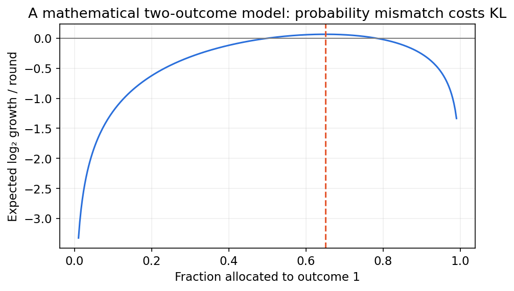
Let outcome occur with probability . Allocate fraction to its contingent payoff, with . A fair reference law pays multiplier when outcome occurs. Then expected base-two log growth is
Here is the outcome law, the allocation, the reciprocal-payoff probability vector, and is log multiplier per trial. The identity uses normalized laws and the stipulated contingent-payoff game [1].
The optimum is on the source support. A mismatched strategy loses exactly expected log growth. For two outcomes with equal multiplier two, is fair and the optimum value is .
This is the Kelly connection between prediction and growth. It does not mean every portfolio has contingent fair payoffs or that probabilities are known. Adding cash, transaction costs, leverage restrictions or different payoffs changes the optimization.
If a side observation is available before each outcome, optimize allocation conditionally. The improvement over a fixed optimal allocation is
Here is the outcome, the side information, and the reference payoff law is unchanged. Mutual information has an operational value in this particular log-growth game.
Universal mixtures connect portfolios with coding
Instead of committing to one fixed allocation, mix the wealth of many fixed strategies. Past outcomes then determine how much each strategy contributes.
For a positive return vector and a fixed simplex allocation , cumulative wealth is
Here indexes trials, has nonnegative entries summing to one, contains each component’s relative payoff, and is a prior measure over fixed allocations. The mixture has an equivalent sequential allocation obtained by weighting strategies by their past wealth.
Cover and Thomas’s Chapter 16 develops universal-portfolio ideas and their long-run comparisons with a best constant allocation under stated conditions [1]. The benchmark is a fixed allocation in hindsight, not an unrestricted future-knowing trader.
For the two-outcome fair contingent game, a uniform prior on the probability parameter yields the same predictive mechanism as a beta mixture. Its sequential probability of one is after observations. This is a whole-count prior, distinct from the half-count predictor in lossless coding.
Code: mixture growth and the best constant allocation
This complete example computes wealth in logarithms and uses the beta integral for the uniform mixture. It compares a known source strategy with the retrospectively best fixed strategy and the causal mixture.
Code · Python · 23 lines
import numpy as np
from scipy.special import betaln

rng = np.random.default_rng(42)
p, n = 0.65, 2000
outcomes = rng.binomial(1, p, size=n)
ones, zeros = int(outcomes.sum()), n-int(outcomes.sum())
fitted = ones/n
oracle_log_wealth = n*np.log(2)+ones*np.log(p)+zeros*np.log(1-p)
best_log_wealth = n*np.log(2)+ones*np.log(fitted)+zeros*np.log(1-fitted)
mixture_log_wealth = n*np.log(2)+betaln(ones+1, zeros+1)
sequential_log_wealth, previous_ones = 0.0, 0
for t, outcome in enumerate(outcomes):
    q = (previous_ones+1)/(t+2)
    sequential_log_wealth += np.log(2*(q if outcome else 1-q))
    previous_ones += int(outcome)
assert abs(sequential_log_wealth-mixture_log_wealth) < 1e-9
assert mixture_log_wealth <= best_log_wealth
print("Source / best fixed / mixture growth bits per trial:",
      oracle_log_wealth/n/np.log(2), best_log_wealth/n/np.log(2),
      mixture_log_wealth/n/np.log(2))
print("Mixture regret to best fixed, bits:",
      (best_log_wealth-mixture_log_wealth)/np.log(2))
This is a controlled synthetic payoff experiment. The best fixed parameter uses the entire sequence and is a benchmark, while the mixture updates causally. Log wealth minus a best benchmark has the same algebra as negative-log-probability regret, with opposite orientation.
Modern view
Hellström, Durisi, Guedj and Raginsky’s published 2025 monograph [3] unifies information-theoretic and PAC-Bayesian generalization bounds. Its taxonomy separates expectation, probability and conditional-mutual-information formulations, making clear that a statistical guarantee needs a specified random object and evaluation criterion.
El Gamal’s 2026 proposed learning chapter [4] connects divergence identities with statistical learning through a textbook-oriented presentation. It is a draft supplement. We use its current perspective alongside the published second edition, without treating a proposed chapter as a completed new edition.
Our inference is that the same quantity can have several operational meanings only after the model is specified. Divergence can be a coding penalty, an unusual-type exponent, an evidence rate or a log-growth loss. The direction, logarithm base and limiting regime can differ among those uses.
Open problems in learned inference include reliable estimation of information in large parameter spaces, guarantees under dependent or shifted data, and bounds that remain informative for actual model selection procedures. A formal inequality can become vacuous when its information term is infinite or difficult to estimate.
For practical work, pair theoretical identities with independent finite experiments: exact toy probabilities to verify implementation, held-out likelihood to assess model fit, and decision-specific errors to evaluate use. No single entropy number replaces all three.
The final chapter combines multiple sources and receivers, develops stronger inequalities, and connects these foundations to modern learning and a small distributed-information capstone.
Key takeaways
- Likelihood evidence, posterior odds and decision thresholds are distinct.
- Testing reports both false-alarm and missed-alternative probabilities.
- Type probabilities have divergence exponents with explicit argument orientation.
- Hypothesis-testing exponents depend on the chosen error regime.
- Sufficiency is relative to a model family and target parameter.
- Fisher information gives local regular-estimation limits.
- Maximum entropy depends on support and stated constraints.
- Log-growth mismatch and universal mixture regret share coding identities.
Exercises
- Reverse the null and alternative in the binomial example. Find a threshold meeting a 5% false-alarm limit and compare the resulting missed-alternative error.
Hint
The rejection region becomes a low-count event.
- Derive the type-probability identity by grouping symbols with equal empirical counts. Explain why the divergence arguments have their displayed order.
Hint
Use counts times log source probability.
- Compare the Stein divergences in both directions for Bernoulli probabilities 0.3 and 0.6. Explain why the asymmetric results do not contradict a symmetric Chernoff exponent.
Hint
Fix the acceptance region before choosing a divergence.
- Reparameterize a Bernoulli probability by log odds. Derive its Fisher information and explain the changed error units.
Hint
Multiply by the squared probability derivative.
- Solve a maximum-entropy distribution on states 0, 1, 2, 3 with mean 1.2. Then add a second-moment constraint and describe the extra multiplier.
Hint
The second feature is squared state.
- In the fair contingent game, calculate expected growth at source probability 0.65 for allocations 0.5, 0.65 and 0.8. Verify the divergence loss and explain which strategy knows future outcomes.
Hint
None knows the future; the hindsight benchmark only fits a constant after observation.
References
-
T. M. Cover and J. A. Thomas, Elements of Information Theory, 2nd ed., Wiley, 2006, Chapters 6, 11–12 and 16. Publisher book and contents.
-
T. Weissman, “Method of Types,” Stanford EE276 Lecture 15 notes, 2024. Primary lecture notes.
-
F. Hellström, G. Durisi, B. Guedj and M. Raginsky, “Generalization Bounds: Perspectives from Information Theory and PAC-Bayes,” Foundations and Trends in Machine Learning, 18(1), 1–223, 2025. Publisher metadata, author version.
-
A. El Gamal, “Information Theory and Statistical Learning,” proposed textbook chapter, arXiv preprint, 2026. Draft and publication status.
-
MIT OpenCourseWare, “Lecture 6: Efficient Estimators, Rao-Cramer Bound,” 14.381 Statistical Method in Economics, Fall 2018, pp. 3–6. Primary lecture notes.
Check your understanding
This tutorial has 6 exercises. Can you solve them without opening the hints?
Go to the exercises ↑Next IT 08 · Networks, Information Inequalities and Learning · 19 min