IT 05 · Differential Entropy and Gaussian Channels
Needs: IT 04 · Channel Capacity and Reliable Communication
Navigate: this page and this track: Navigate: this page and this track
On this page
- What you’ll learn1 min
- The big picture1 min
- A density is not a point probability1 min
- Quantization explains the relationship to actual symbols1 min
- Coordinate changes alter differential entropy2 min
- Relative entropy and mutual information remain meaningful1 min
- Gaussian distributions maximize entropy at fixed covariance2 min
- Derive the real Gaussian-channel capacity1 min
- A geometric view and its limits1 min
- Parallel channels and water-filling2 min
- Vector channels connect geometry with covariance1 min
- Conditional entropy and deterministic representations2 min
- Modeling and estimation: what the formulas certify1 min
- Modern view1 min
- Key takeaways1 min
- Exercises1 min
- References
Information Theory
Explore this chapter 1 interactive experiment
Compare equal allocation with water-filling across two parallel Gaussian channels.
What you’ll learn
- Define differential entropy without treating a density as a probability.
- Track units and coordinate changes while preserving mutual information.
- Derive the Gaussian maximum-entropy property from relative entropy.
- Obtain real Gaussian-channel capacity under an average-power budget.
- Allocate power across parallel channels through water-filling.
- Distinguish analytical information limits from estimation and implementation costs.
The big picture
An amplitude can take a continuum of values, but a receiver with noise cannot distinguish infinitely many messages for free. More precise measurements require more resources, and a transmitter cannot generally use arbitrarily large amplitudes. Continuous information theory keeps those constraints visible.
This chapter follows Cover and Thomas’s Chapters 8–9 [1], supplemented by Stanford’s continuous-variable and Gaussian-channel notes [2,3]. The progression matters: we first define density-based information, then prove a distributional bound, then use it to optimize communication under a power constraint.
Continuous formulas also appear in vision features, latent representations and sensor noise models. Their numerical values can change under a change of units even when the scene has not changed. Mutual information is the more stable object for comparing relationships.
A density is not a point probability
A continuous density describes probability per unit of measurement. A density value above one is perfectly possible and does not violate probability rules.
For a real random variable with density ,
Here is a measurable region, is a coordinate in the chosen units, and is density rather than the probability of the exact point. Under an ordinary continuous density, each exact point has probability zero.
A uniform variable on an interval of width one tenth has density ten on that interval. Its probability over the whole interval is still one. Taking the negative logarithm of a density can therefore yield a negative value.
The differential entropy is
Here is differential entropy in base-two units and the integral is taken where the density is defined. The expression assumes the integral exists in the relevant sense. It can be negative or infinite, and some distributions have no well-defined finite entropy.
Unlike discrete entropy, differential entropy alone is not a minimum count of bits needed for exact representation of a continuously distributed value. Exact infinite-precision reconstruction is a different, generally unbounded requirement.
The notation deliberately uses lowercase for differential entropy and uppercase for discrete entropy. They share algebraic relationships under appropriate conditions, but their interpretation and sign constraints differ.
Quantization explains the relationship to actual symbols
A real instrument records bins, not infinitely precise points. As bins shrink, describing the bin index costs more bits.
Quantize a scalar density into bins of width . For a sufficiently regular density and fine quantization,
Here is the discrete bin index, is measured in the same coordinate units as , and the approximation is a fine-bin asymptotic relationship subject to regularity and tail conditions.
Each bin probability is approximately density times bin width. Its negative log-probability is therefore approximately negative log-density minus log-width. Averaging gives the formula.
The extra term is not a small correction. It diverges as resolution increases. A finite differential entropy does not make arbitrarily precise values cheap to encode.
At coarse resolution, sharp discontinuities or heavy tails, the approximation may be poor. Real quantizers may have saturation, nonuniform bins or a finite range. These details change the discrete distribution and must be included in an actual coding experiment.
For a sensor, both resolution and physical noise matter. Increasing stored numerical precision beyond measurement precision need not create new information about the scene. It can merely create more digits representing uncertain amplitudes.
Code: coordinate units and quantized entropy
This standalone experiment uses a unit uniform variable, computes empirical bin-index entropy at different resolutions, and compares an analytic differential-entropy change under scaling.
Code · Python · 18 lines
import numpy as np

rng = np.random.default_rng(36)
x = rng.uniform(0, 1, size=100000)
def discrete_entropy(values):
    _, counts = np.unique(values, return_counts=True)
    p = counts / counts.sum()
    return -np.sum(p * np.log2(p))
for bins in [10, 100, 1000]:
    indices = np.floor(x * bins).astype(int)
    estimated = discrete_entropy(indices)
    theoretical = np.log2(bins)
    print("Bins / estimated index entropy / exact:", bins, estimated, theoretical)
    assert abs(estimated - theoretical) < 0.03
scale = 0.1
h_x, h_scaled = 0.0, np.log2(scale)
print("Differential entropy before / after scaling:", h_x, h_scaled)
assert h_scaled < 0
The negative scaled entropy is not negative uncertainty in a discrete message. It reflects density per coordinate unit. The finite bin estimate remains nonnegative and has sampling bias that grows when there are many rare bins.
Coordinate changes alter differential entropy
Measuring the same length in millimeters instead of meters stretches the numerical distribution. Differential entropy changes with that stretching.
For a nonzero scalar and translation ,
Here scales coordinates and translates them. A translation does not alter density volume; scaling multiplies it by . For an invertible matrix applied to a -dimensional vector,
Here is a nonsingular by matrix, a translation vector, and its determinant. Both sides require well-defined entropies.
A smooth one-to-one nonlinear coordinate map has the corresponding Jacobian correction:
Here is the derivative matrix of , evaluated at random , and the expectation averages its log-volume change. This identity requires appropriate differentiability, invertibility and integrability.
It explains why latent density values depend on representation coordinates. An invertible transformation can change differential entropy without discarding information. Comparing two feature spaces by raw differential entropy alone can confuse coordinate expansion with information quality.
Derive the scale correction from the density
The correction can be understood directly rather than memorized. Let with . Probability is preserved under the coordinate change, so
Here is the transformed variable, its coordinate, its density, and are scale and translation. Density decreases by when the coordinate interval expands by that factor. Consequently its negative log-density gains the constant . Averaging over the unchanged event probabilities gives the entropy correction.
Take a uniform source on an interval of width 0.1. Its differential entropy is . Quantize it into ten equal bins of width 0.01: each bin has probability one tenth, and the discrete entropy is bits. Here the fine-bin relationship is exact because the density is constant and the bins align with the support.
Change units by multiplying all coordinates by 100. The interval width becomes ten, differential entropy becomes , and bin width becomes one. The same ten outcomes still cost 3.321928 bits. Scaling changes the density entropy and bin-width correction in opposite directions; it does not create additional distinguishable events. Changing only the number of bins would change the observation, whereas changing coordinate units does not.
Relative entropy and mutual information remain meaningful
Comparing densities by a ratio cancels shared coordinate units. A relationship between two variables should not disappear when either is measured in a different reversible coordinate system.
For densities and ,
Here is a joint density and is the independent product reference. Divergence is nonnegative, with an infinite value when support or integrability demands it.
Under separately invertible coordinate changes of and , the Jacobian factors cancel in the density ratio and integral, so mutual information is unchanged. This statement does not apply to a noninvertible projection or quantization; those can discard information and are governed by data processing.
When all entropies are finite and compatible,
Here is joint differential entropy and is expected conditional differential entropy. Conditional differential entropy may be negative. The resulting mutual information remains nonnegative.
The density-ratio definition is safer when entropy differences would subtract infinities. A noiseless deterministic identity between genuinely continuous variables can have infinite mutual information and a singular joint law; ordinary full-dimensional joint-density formulas then need care.
For a jointly Gaussian scalar pair with correlation ,
Here is the correlation coefficient and makes covariance nonsingular. Correlation is sufficient for this formula only under joint Gaussianity; a general dependence cannot be summarized by one covariance number.
Gaussian distributions maximize entropy at fixed covariance
Among distributions with a specified covariance, a Gaussian spreads uncertainty most broadly in the differential-entropy sense. This is a constrained statement, not a claim that every source is Gaussian.
A nonsingular -dimensional Gaussian with covariance has
Here is the Gaussian vector, its dimension, its positive-definite covariance, and the base of natural logarithms. Its mean does not affect entropy.
For another density with the same mean and covariance, compare it with Gaussian density . The Gaussian log-density is a constant plus a quadratic form. Its expectation under equals its expectation under because the first two moments match. Thus
Here has density , and the equality assumes the needed finite quantities. It proves the maximum-entropy property and identifies equality with the Gaussian distribution [1,2].
In one dimension, fixed variance gives maximum entropy . Specifying only support gives a different extremizer: a uniform density on that bounded support. Constraints determine the maximum-entropy distribution.
This proof is valuable beyond communication. It makes a modeling choice transparent: adopting a Gaussian from a mean and covariance adds no further shape constraint in the maximum-entropy formulation. It does not certify the fit, rule out multimodality or make a Gaussian likelihood robust to outliers.
The covariance must be symmetric positive definite, not merely have a positive determinant: has determinant one but negative variances, where is the two-dimensional identity matrix. The code checks symmetry explicitly, then uses a Cholesky factor to obtain the log-determinant [6]. A singular covariance describes a lower-dimensional Gaussian law; adding diagonal noise would define a different model, so this full-dimensional entropy routine rejects it.
Code: Gaussian information and reversible scaling
The complete example estimates covariance from a synthetic Gaussian pair, computes its Gaussian-model information, and verifies that an invertible scaling changes entropy while preserving the information formula.
Code · Python · 39 lines
import numpy as np

rng = np.random.default_rng(37)
rho = 0.7
covariance = np.array([[1, rho], [rho, 1]])
samples = rng.multivariate_normal([0, 0], covariance, size=100000)
estimated_cov = np.cov(samples, rowvar=False)
def gaussian_entropy(cov):
    cov = np.atleast_2d(np.asarray(cov, dtype=float))
    if (cov.ndim != 2 or cov.shape[0] != cov.shape[1]
            or not np.all(np.isfinite(cov))
            or not np.allclose(cov, cov.T, rtol=0, atol=1e-12)):
        raise ValueError("Covariance must be a finite symmetric square matrix")
    factor = np.linalg.cholesky(cov)  # rejects singular or indefinite inputs
    logdet = 2*np.log(np.diag(factor)).sum()
    d = cov.shape[0]
    return 0.5 * (d * np.log(2*np.pi*np.e) + logdet) / np.log(2)
def gaussian_information(cov):
    return (gaussian_entropy([[cov[0, 0]]]) +
            gaussian_entropy([[cov[1, 1]]]) - gaussian_entropy(cov))
# A positive determinant alone is not a covariance-validity check.
assert np.linalg.det(-np.eye(2)) > 0
for invalid in [-np.eye(2), np.ones((2, 2)), [[1., 1.], [0., 1.]]]:
    try:
        gaussian_entropy(invalid)
    except (ValueError, np.linalg.LinAlgError):
        pass
    else:
        raise AssertionError("Invalid covariance was accepted")
estimated = gaussian_information(estimated_cov)
exact = -0.5 * np.log2(1-rho**2)
transform = np.diag([100, 0.2])
scaled_cov = transform @ estimated_cov @ transform.T
assert abs(gaussian_information(scaled_cov) - estimated) < 1e-12
assert abs(gaussian_entropy(scaled_cov) - gaussian_entropy(estimated_cov)
           - np.log2(abs(np.linalg.det(transform)))) < 1e-12
assert abs(estimated - exact) < 0.02
print("Estimated Gaussian-model MI / exact MI:", estimated, exact)
print("Entropy shift:", gaussian_entropy(scaled_cov) - gaussian_entropy(estimated_cov))
This is a Gaussian parametric calculation, not a general-purpose mutual-information estimator. On a non-Gaussian dataset, plugging in covariance answers a Gaussian-model question and can miss substantial nonlinear dependence.
Derive the real Gaussian-channel capacity
Signal power increases the spread of distinguishable outputs; noise blurs them. The capacity depends on their ratio, under the precise Gaussian model.
Consider one real amplitude per use:
Here is the input, the output, independent zero-mean Gaussian noise, noise variance, average input power, and denotes independence. Across uses the noise is independent with the same law.
Conditioning on leaves only translated noise, so . Output variance is at most . Gaussian maximum entropy therefore yields
Here is the signal-to-noise ratio. Independent Gaussian input makes the output Gaussian and attains this single-letter bound. The corresponding coding theorem establishes
bits per real channel use under the standard average-power model [1,3]. The maximizing input has zero mean because a deterministic mean consumes power without increasing distinguishable variation.
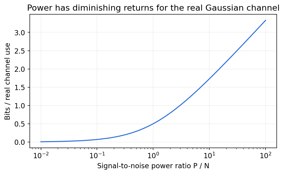
An average-power constraint does not impose a strict maximum on every amplitude. Adding a peak-amplitude constraint changes the optimizing input distribution and generally the value. A finite constellation also defines a more restricted signaling problem.
The analogous complex-valued formula often lacks the one-half factor because a complex use includes two real dimensions, under a corresponding noise and power convention. Comparing the expressions without defining a use can create a false factor-of-two improvement.
A geometric view and its limits
Over many uses, noise places the observation in a cloud around the transmitted codeword. Good codewords are far enough apart that the clouds are usually distinguishable.
For independent Gaussian noise samples, squared norm concentrates near :
Here is noise at use , and the arrow denotes the appropriate law-of-large-numbers convergence. Power-constrained codewords lie near an input radius on the scale , while outputs occupy a larger scale involving .
Comparing high-dimensional output volume with noise-cloud volume suggests a count on the scale , whose normalized binary logarithm is the capacity expression. This is a geometric explanation, not an assertion that Gaussian noise has bounded support.
Noise can leave any finite sphere with positive probability. Reliable communication requires that atypical observations become sufficiently rare, not that noise clouds are literally disjoint for every possible outcome. That distinction separates vanishing-error capacity from zero-error communication.
The geometry also explains why a one-use diagram can be misleading. Long blocks allow many coordinates to cooperate, and their aggregate norms concentrate. A short-block constellation has its own distance and decoding tradeoffs.
Parallel channels and water-filling
When several independent channels have different noise levels, distribute power where it creates the greatest marginal increase in information. Some very noisy channels may receive no power.
For parallel real Gaussian channels with variances , allocate powers under total :
Here indexes one parallel dimension, is their count, and the objective is bits per joint use of all dimensions. Independent Gaussian inputs attain the component rates.
The derivative with respect to an active power is . Equalizing derivatives under a common budget yields
Here is the water level and . The notation reflects filling above noise floors: active channels reach a common total signal-plus-noise level.
This follows from the optimality conditions of a concave optimization problem. A channel whose noise floor exceeds the level receives zero; assigning it positive power would give a smaller marginal return than an active lower-noise channel.
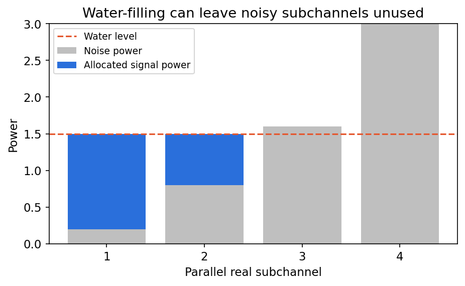
Solve the plotted allocation by hand
The noise floors are 0.2, 0.8, 1.6 and 3.0, and the total signal-power budget is two. First suppose only the first channel is active. Its total level would be , which rises above the second floor. Leaving the second channel unused cannot be optimal.
Try the first two active channels. Their powers sum to , giving . This is above both active floors and below the next floor 1.6, so the assumed active set is consistent. Allocate powers 1.3, 0.7, zero and zero.
The resulting joint-use rate is bits. Equal allocation of 0.5 to each channel gives about 1.561252 bits. Both designs spend total power two; the improvement comes from its placement, not an enlarged budget.
The third channel becomes active when the level exceeds 1.6, which first requires budget . The fourth becomes active above level three, at budget . These thresholds explain the changing active set in a capacity–power curve.
Equal signal-plus-noise levels apply only to the active channels. A channel with a floor above the level keeps zero signal power. This complementary condition is why blindly forcing equal total levels across all four channels would produce impossible negative powers.
Code: solve the level and compare equal allocation
This complete example solves the level by bisection, verifies the budget and active optimality condition, and compares its rate with equal power.
Code · Python · 20 lines
import numpy as np

noise = np.array([0.2, 0.8, 1.6, 3.0])
budget = 2.0
low, high = noise.min(), noise.max() + budget
for _ in range(100):
    level = (low + high) / 2
    if np.maximum(level-noise, 0).sum() > budget:
        high = level
    else:
        low = level
level = (low + high) / 2
power = np.maximum(level-noise, 0)
equal = np.full(len(noise), budget / len(noise))
rate = lambda allocation: 0.5*np.log2(1+allocation/noise).sum()
assert abs(power.sum()-budget) < 1e-12
assert np.allclose(noise[power > 0]+power[power > 0], level)
assert rate(power) >= rate(equal)
print("Water level / power allocation:", level, power)
print("Water-filled / equal-allocation joint rate:", rate(power), rate(equal))
The objective counts one simultaneous use of every dimension. Dividing by the number of dimensions gives a different per-dimension average. Neither number becomes bits per second until a use rate is supplied.
With colored Gaussian noise, a covariance eigenbasis can create parallel noise modes under compatible linear input and power assumptions. With channel gains, the effective noise floor depends on gain as well as physical noise. A zero gain cannot be inverted into a useful channel.
Vector channels connect geometry with covariance
Several measurements can carry overlapping information about several input coordinates. A matrix describes mixing, while covariance describes the noise cloud and the chosen signal spread.
Consider the real linear channel
Here is a -dimensional input, an -dimensional output, an by channel matrix, an input covariance and a positive-definite noise covariance. The input covariance can be positive semidefinite, allowing unused directions.
The output covariance is . Subtracting Gaussian output and conditional noise entropies gives
Here is the matrix transpose and determinants refer to output-dimensional covariance matrices. The positive noise covariance keeps the denominator and output covariance nonsingular, even if the signal has lower rank.
Under an average total-power convention, constrains the sum of input coordinate variances. Maximizing the displayed information over positive-semidefinite gives the corresponding Gaussian vector-channel problem [1]. The trace notation means the sum of diagonal entries, and is total power per vector use.
The useful directions depend jointly on and . A large raw coordinate variance may lie in a direction strongly attenuated by the channel. Correlated noise may make a direction less informative than its marginal variance suggests. Diagonalizing a compatible transformed problem reveals parallel modes where the same marginal-return principle applies.
This example makes clear why preprocessing and physical channel changes must be distinguished. An invertible receiver coordinate transform changes both the signal matrix and the noise covariance; the determinant ratio stays invariant. A projection discards output directions and can reduce information. A noninvertible transmitter map changes which input signals can be produced.
For numerical work, compute log-determinants with a stable factorization instead of taking a large determinant and then its logarithm. A huge determinant can overflow while its logarithm is moderate. Check positive definiteness and matrix dimensions before interpreting the answer.
Conditional entropy and deterministic representations
A representation can be numerically continuous but carry only a finite set of possible states. Its mathematical distribution depends on how it was created, not the array’s floating-point storage type.
The differential-entropy definitions assume densities with respect to continuous coordinate volume. A discrete label stored as a floating-point number remains discrete. A vector produced by a deterministic map of a finite dataset has finite empirical support, even if its coordinates are real-valued.
A lower-dimensional manifold inside a larger feature space has a singular distribution relative to full-dimensional volume. Fitting a full-dimensional density implicitly introduces a noise or smoothing model. The resulting entropy belongs to that model and can depend strongly on its scale.
Likewise, adding tiny independent noise to a deterministic continuous relationship makes a density-based calculation possible, but the noise level becomes part of the information question. Letting that level approach zero can send mutual information to infinity. Reporting a finite value without the smoothing convention hides this dependency.
These observations are useful when comparing neural representations. The information relevant to a discrete task label can remain finite, while information between an exactly deterministic continuous input and representation can be singular. A compression or predictive objective must specify which variables, noise mechanisms and quantizers define its rate.
The practical remedy is to state the observation model before estimating information: discrete bins, an explicit noisy channel, a parametric density or a fixed-resolution coding protocol. Each is legitimate for its stated purpose, and each answers a different question.
Why vanishing added noise can make information diverge
Consider and representation , where independent noise has positive variance . This is a Gaussian channel with signal power one, so . With , information is one half bit. With , it is approximately 3.329106 bits. As noise variance tends to zero, the number grows without bound.
At exactly zero noise, is an exact continuous copy. The pair lies on a line in the two-dimensional joint space, so it has no ordinary two-dimensional joint density. This is why directly subtracting marginal and joint differential entropies at that endpoint is unsafe. Finite-resolution bins would instead give a finite discrete information question. The noise or resolution convention determines which question a neural-representation estimate answers.
Modeling and estimation: what the formulas certify
A Gaussian formula certifies a Gaussian problem. It does not convert every covariance estimate into a reliable physical communication limit.
The scalar capacity derivation uses independent additive Gaussian noise, an average second-moment budget and an unbounded real input alphabet. A sensor with clipping, quantization, signal-dependent noise or a changing noise distribution may violate one or more assumptions.
For a bounded output quantizer, information cannot exceed the logarithm of its number of possible labels. A real-valued capacity formula calculated before quantization is an upper reference for a different observation model; it is not automatically attainable by the quantized receiver.
Likewise, using a Gaussian approximation for a non-Gaussian source’s entropy produces a moment-based upper bound under the needed conditions. It is not a measured entropy value. Good agreement of means and covariances does not establish agreement of tails or dependence.
Finite sample estimates of covariance can be singular when dimension is too high relative to observations. Then a log-determinant formula may fail. Regularizing the covariance creates a modified statistical model; the regularization value affects the reported information and should be stated.
For evaluation, keep the physical noise model, coordinate convention, estimated parameters and observed decoder performance separate. A synthetic test can verify algebra and implementation, while independently collected data must verify the assumptions.
Modern view
Butakov and colleagues’ NeurIPS 2024 paper [4] studies mutual-information estimation through normalizing-flow transformations. It provides a modern example of using invertible density models to help estimation, while retaining the need to assess the estimator rather than interpreting coordinate entropy as intrinsic information.
The review perspective in contemporary semantic-communication literature [5] distinguishes receiver modeling, generative reconstruction and learned joint coding. For continuous channels, our inference is that those designs should report power normalization, real or complex use conventions, receiver quantization and channel mismatch explicitly.
An attractive reconstructed image can coexist with low faithful information about a particular original detail. A task-based objective may intentionally discard that detail; this is a rate–distortion choice rather than a different differential-entropy convention.
Open problems include robust information estimation in high dimension, evaluating likelihood models under shift, handling finite precision consistently at both endpoints, and designing learned systems whose resource accounting matches the physical channel. Invertibility and Gaussian assumptions simplify mathematical analysis, but neither substitutes for those checks.
The next chapter asks how much source information is needed when some reconstruction error is acceptable. Gaussian capacity concerns transporting information; Gaussian rate–distortion concerns how much information the source demands.
Key takeaways
- Density is probability per coordinate unit, not a point probability.
- Differential entropy can be negative and changes under coordinate scaling.
- Fine quantization adds a resolution-dependent discrete description cost.
- Relative entropy and mutual information survive reversible coordinate changes.
- Gaussian maximum entropy is a consequence of fixed moment constraints.
- Real Gaussian capacity includes an explicit average-power budget and one-half factor.
- Water-filling equalizes marginal returns across active parallel channels.
- Parametric information formulas and empirical decoder reliability answer different questions.
Exercises
- Find the differential entropy of a uniform variable on an interval of width 0.01. Explain why its negative value does not permit a negative-length code.
Hint
Use log interval width and separate bin coding.
- Quantize a unit uniform source into 16, 64 and 256 equal bins. Compute exact discrete entropy and relate it to differential entropy.
Hint
Each bin is equiprobable.
- Verify mutual-information invariance under separate nonzero scalings of a jointly Gaussian pair. What changes if one variable is rounded to a single bit?
Hint
Determinants cancel for reversible scales; rounding is not invertible.
- Compare capacity gains from doubling power at signal-to-noise ratios 0.1 and 10. Explain why absolute rate increments behave differently from relative power increments.
Hint
Subtract capacities before and after doubling.
- Increase the water-filling budget until the third and fourth channels become active. Calculate the activation thresholds from the noise floors.
Hint
Set the water level to the next noise floor.
- Explain which assumptions fail for a clipped receiver with two output labels. Give an information upper bound independent of signal power.
Hint
Output entropy is at most one bit.
References
-
T. M. Cover and J. A. Thomas, Elements of Information Theory, 2nd ed., Wiley, 2006, Chapters 8–9. Publisher book and contents.
-
T. Weissman, “Continuous Random Variables,” Stanford EE276 Lecture 8 notes, 2024. Primary lecture notes.
-
T. Weissman, “AWGN Channel,” Stanford EE276 Lecture 9 notes, 2024. Primary lecture notes.
-
I. D. Butakov, A. D. Tolmachev, S. V. Malanchuk, A. M. Neopryatnaya and A. A. Frolov, “Mutual Information Estimation via Normalizing Flows,” NeurIPS, 2024. Published paper.
-
L. X. Nguyen, A. D. Raha, P. S. Aung, D. Niyato, Z. Han and C. S. Hong, “A Contemporary Survey on Semantic Communications: Theory of Mind, Generative AI, and Deep Joint Source-Channel Coding,” IEEE Communications Surveys & Tutorials, 2025. Published-paper metadata and author version.
-
NumPy developers, “numpy.linalg.cholesky,” NumPy documentation, accessed 2026-11-05. Official API documentation.
Check your understanding
This tutorial has 6 exercises. Can you solve them without opening the hints?
Go to the exercises ↑Next IT 06 · Rate–Distortion and Lossy Representations · 18 min