IT 08 · Networks, Information Inequalities and Learning
Needs: IT 07 · Statistical Evidence, Maximum Entropy and Growth
Navigate: this page and this track: Navigate: this page and this track
On this page
- What you’ll learn1 min
- The big picture1 min
- Distributed source coding: correlation can save rate3 min
- Multiple access: independent messages share one output2 min
- Broadcast and relay channels change the information pattern1 min
- Joint usefulness can be invisible to marginal information2 min
- Stronger inequalities extend the toolkit1 min
- Entropy power and added Gaussian noise1 min
- Representation information and sample information3 min
- Capstone: side-information decoding with parity bins1 min
- Modern view2 min
- A reading and project path after the course1 min
- Key takeaways1 min
- Exercises1 min
- References
Information Theory
Explore this chapter 1 interactive experiment
Compute information about a noisy XOR label from each independent bit and from their pair.
What you’ll learn
- Describe rate regions for distributed sources and multiple-access channels.
- Explain why broadcast, relay and general networks need different arguments.
- Apply log-sum, Pinsker, entropy-power and conditional-information inequalities.
- Distinguish representation information from information about a training sample.
- Run a small distributed parity-code decoder with explicit finite errors.
- Connect the book’s complete chapter map to current learning research without overstating limits.
The big picture
One sender and one receiver lead to a single capacity. Several sources or receivers lead to a region of compatible rates. Improving one rate may reduce another, and information can be useful jointly even when each component looks useless alone.
This final tutorial follows Cover and Thomas’s Chapter 15 on networks and Chapter 17 on inequalities [1]. Earlier chapters covered the other fifteen book chapters through the reading map in IT 01. We end with a finite synthetic experiment that connects source dependence, coding, decoding and task information.
The course uses the published second edition, supplemented by current surveys and a clearly labeled 2026 proposed chapter.
Distributed source coding: correlation can save rate
Two encoders can separately describe correlated observations while a joint decoder uses their relationship. The encoders need not each send every bit independently.
Let independent pairs follow a fixed finite joint law. Encoder one observes only , encoder two only , and a common decoder reconstructs both blocks. The Slepian–Wolf asymptotically almost-lossless region is
Here are bits per paired source sample sent by the separate encoders, and the entropies use the specified joint source. Boundary inequalities describe the closure; codes operate with suitable rate margins and vanishing block error [1].
The individual bounds assume the other source can help at decoding. The sum bound counts total joint uncertainty. Neither encoder is assumed to see the other’s current block; allowing that observation would define a different problem.
For fair and with independent Bernoulli noise probability , both marginal entropies are one and joint entropy is . Separately ignoring dependence would require two bits per pair asymptotically; joint decoding can exploit the smaller joint uncertainty.
One corner sends at its full marginal rate and compresses toward . The decoder already has the reconstructed , which acts as side information. This corner motivates the parity-syndrome experiment below.
Random binning supplies an existence argument: assign source blocks to bins and use the other decoded source to find the likely matching block in the signaled bin. The bin index tells less than a full source index, while the correlation resolves ambiguity.
This result is not exact reconstruction of every possible finite pair. Rare or ambiguous blocks can fail. Truly lossless finite protocols require an additional escape or other treatment if every allowed realization must be recovered.
Why random bins produce three rate constraints
Each encoder randomly assigns every possible source block to a bin and sends its bin index. The decoder searches for a jointly typical pair in the two indicated bins. A competing pair can be wrong in three ways: only X is wrong, only Y is wrong, or both are wrong.
| Competing pair | Typical candidate count scale | Collision probability per candidate |
|---|---|---|
| Wrong X, correct Y | ||
| Correct X, wrong Y | ||
| Both wrong |
Here is paired block length, the sent bin-index rates, and the entropy exponents use the fixed joint source. These scales omit the small typicality tolerances and finite prefactors. Independent bin assignments give the collision factors, while joint typicality limits how many candidates need consideration.
Multiply each count by its collision probability and use a union bound. All three terms vanish with suitable margins exactly when the two individual rates exceed their conditional entropies and their sum exceeds joint entropy. The true pair fails typicality with a probability that also vanishes. Averaging over assignments then proves some fixed shared binning rule has small block error [1].
This proof explains both the correlation gain and its limit. Decoder side information reduces the number of candidate X blocks from the full source catalog to a conditional catalog. It does not eliminate the need to distinguish the remaining candidates. The sum constraint handles simultaneous ambiguity that neither individual bound can remove alone.
For fair bits with flip probability 0.1, conditional entropy is about 0.468996 and joint entropy 1.468996 bits per pair. The corner rates are approximately and . A symmetric point has rate 0.734498 for each encoder; assigning 0.5 to each passes the individual bounds but fails the sum bound. These are limiting boundary values, so actual asymptotic constructions use margins rather than promising a short-block code at the boundary.
Multiple access: independent messages share one output
Two senders can both communicate through a common receiver. The receiver’s observation limits their combined information as well as each individual rate.
For a finite memoryless channel with independent messages, the region for a fixed product input law includes
Here are sender inputs, the shared output, and bits per common channel use. Union over product input laws and time-sharing gives the ordinary two-user multiple-access capacity region [1].
Conditioning in an individual bound reflects the receiver being able to distinguish that user’s message when the other input is known. The sum bound addresses joint decoding. Maximizing each individual expression separately does not remove the shared sum constraint.
Time-sharing introduces a common predetermined variable and product inputs given . The corresponding bounds condition each expression on , and convexify operating points. The senders do not gain arbitrary message-dependent cooperation simply because they share a schedule.
For independent real Gaussian signals with powers and additive noise variance ,
Here one use contains both simultaneous real inputs; the signals have independent messages and the standard average-power constraints. The one-half factors retain the real-valued convention.
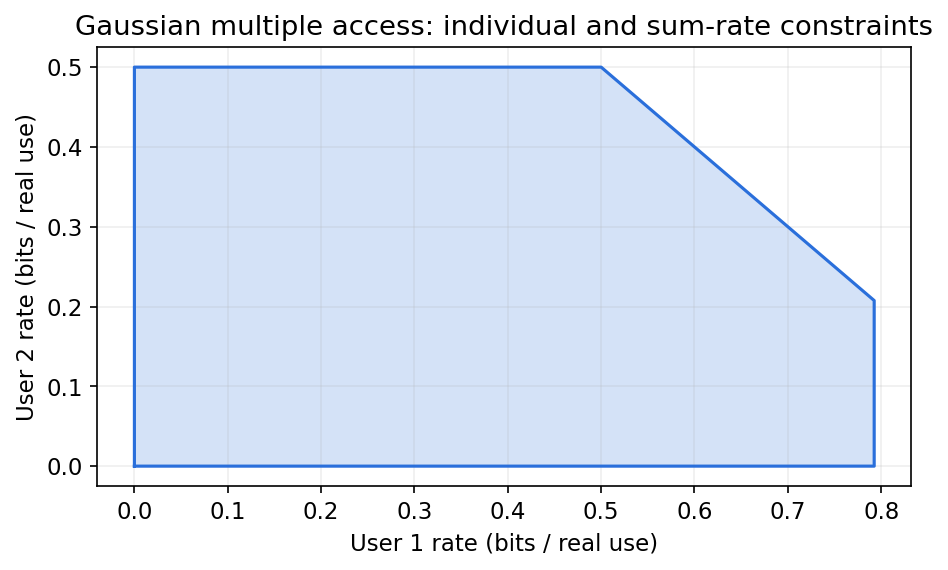
Successive decoding can achieve corner points by first decoding one message while treating the other as noise, then removing the decoded contribution. The order changes which user receives the more favorable conditional rate. Joint decoding and time-sharing describe the broader region.
Work through the two Gaussian decoding orders
For the figure’s powers , and noise variance , user one’s individual bound is about 0.792481 bits per use, user two’s is 0.5, and the shared sum bound is one. The pair satisfies both individual bounds but violates the sum. The pair satisfies all three.
Decode user one first. Its decoder initially treats user two’s independent Gaussian signal as additional noise of variance one, so its rate is limited to . After successful decoding and subtraction, user two sees only the original noise and reaches 0.5. This order gives corner .
Decode user two first instead. Its initial rate is . After removing that signal, user one reaches . This gives corner . Both corners have total rate one, but decoding order allocates that total differently.
The subtraction argument assumes the first message was decoded correctly. A wrong first decision can propagate to the second, so a finite receiver must measure joint message error as well as individual errors. The asymptotic corner calculation guides design without hiding that implementation issue.
Broadcast and relay channels change the information pattern
One sender with two receivers is not the reverse of two senders with one receiver. A relay that hears and retransmits creates another distinct pattern.
In a physically degraded broadcast channel, makes receiver one stronger in the specified statistical sense. A superposition construction uses an auxiliary variable with :
Here is the weaker receiver’s private-message rate, the stronger receiver’s private-message rate, and the layer both can resolve. Union over appropriate gives the degraded-channel capacity region [1].
The Markov order is an assumption about receiver observations, not simply a ranking by sample accuracy. A general broadcast channel need not be degraded and does not inherit this exact region.
For a memoryless relay, let source input be , relay input , relay observation and destination observation . A cut-set upper bound is
Here the first cut separates the source from relay plus destination; the second separates source plus relay from the destination. The input joint law in the upper bound permits statistical cooperation as an outer relaxation.
A cut-set bound is not automatically achievable. Relays may decode a message, describe an observation, or use other causal strategies, each with its own conditions. General network capacity remains unresolved in many settings.
The lesson is to draw the actual information pattern before applying a formula: independent messages, correlated sources, side observations, causal relays and receiver demands are different assumptions. A scalar point-to-point capacity cannot summarize all of them.
Joint usefulness can be invisible to marginal information
Two individually uninformative features can jointly determine a target. Ranking only one feature at a time may discard both.
Let be independent fair bits and . Then
Here is the binary exclusive-or target. Each marginal input leaves the target fair; knowing both gives an exact answer. Conditioning on the other input reveals the first one’s full relevance.
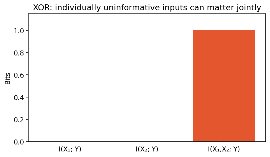
The word synergy is useful informally for this joint-only information, but a general quantitative redundancy–synergy decomposition requires an additional definition. The three mutual-information values alone do not define a universal decomposition for arbitrary variables.
This matters for multimodal learning. A modality that seems weak by itself may be useful in context. Conversely, two strong marginal features may carry largely overlapping information. Analyze the actual joint law and receiver task rather than equating marginal relevance with unique contribution.
Computing a function is another distributed problem
Suppose separate encoders observe independent fair blocks and , and the decoder needs only their coordinatewise exclusive-or. The output has one bit of entropy per pair. It is tempting to conclude that one total bit per pair must suffice.
That conclusion ignores who sees the inputs. Give the decoder the second raw block as extra information. If it can recover the exclusive-or from the two transmitted indices, it can then recover the first block. The second encoder’s index supplies no additional first-block information because the inputs are independent.
Consequently the first encoder must convey approximately one bit per coordinate for vanishing error in this example. By symmetry, so must the second. The distributed sum requirement can therefore be two bits even though the desired function has entropy one.
If one central encoder observed both inputs, it could instead transmit the exclusive-or itself at one bit per pair. The target is unchanged, but the observation pattern differs. This is a concrete reason to keep the network diagram beside a task-oriented rate claim.
The example also separates two meanings of “joint information.” The receiver may need a joint computation, while the senders lack joint observation. A learned system cannot assume a centrally available feature merely because that feature would be sufficient after it had been computed.
Real applications can have correlated inputs, interaction, common randomness or additional side information, each changing the problem. Do not transfer the independent noninteractive example’s rate conclusion to those settings without deriving the corresponding constraints.
Stronger inequalities extend the toolkit
Information inequalities often compare what remains after merging outcomes, changing a distribution, or adding independent noise. Their units and assumptions decide what they imply.
For nonnegative numbers and positive , the log-sum inequality states
Here indexes entries, are their sums, and zero terms use the standard continuous convention. The all-zero case has both sides zero. This inequality underlies divergence convexity and aggregation forms of data processing [1].
Applying it inside each cell of a partition shows that merging outcomes cannot increase relative entropy. Fine measurements can distinguish distributions in ways a coarse summary no longer reveals.
For finite probability vectors , Pinsker’s inequality gives
Here total variation bounds differences in event probabilities, and divergence uses natural logarithms. If divergence is reported in bits, multiply it by inside the square root. A small divergence therefore controls event-probability differences, while large divergence can make the bound uninformative.
Discrete entropy is also submodular:
Here are sets of variable indices, is the corresponding collection, and the empty collection has entropy zero. The difference is a conditional mutual information between the nonoverlapping parts given the intersection, so it is nonnegative.
This is a relation among entropies of subsets, not a statement that every task-relevance function is submodular. The XOR target is a useful reminder that feature information can increase when another feature is supplied.
Entropy power and added Gaussian noise
Differential entropy can be converted into a variance-like quantity. Adding independent continuous signals cannot make their combined entropy power smaller than the sum.
For a -dimensional vector with finite natural-unit differential entropy, define entropy power
Here is dimension and uses natural logarithms. A scalar Gaussian has entropy power equal to its variance; an isotropic Gaussian vector has the common coordinate variance.
The entropy-power inequality for independent vectors of the same dimension states
Here must satisfy the relevant density and finiteness assumptions. Equality holds for independent Gaussian vectors with proportional covariance matrices in the standard nondegenerate setting [1].
The de Bruijn identity connects noise smoothing with Fisher information:
Here is an independent standard Gaussian vector, is noise variance per coordinate, and is location Fisher information. Smoothness and integrability conditions are required.
This Fisher information is a density-gradient quantity related to location estimation, not an arbitrary parameter’s Fisher information from the previous chapter. Keeping that definition explicit avoids confusing two similarly named objects.
Adding noise can increase observation entropy while reducing information about the original. There is no contradiction: entropy power concerns output spread; data processing concerns retained relationships. Modern noisy representation models must distinguish those two claims.
Representation information and sample information
A feature can preserve a target while limiting raw input detail. A trained model can also reveal how much it depends on a particular training sample. These are different information questions.
An information-bottleneck objective for is
Here is the observation, the chosen relevance target, a possibly stochastic representation, and balances compression against target information. Goldfeld and Polyanskiy’s published tutorial [2] develops this theory and its learning connections.
The objective selects a task-relative statistical representation. It does not establish that every neural network spontaneously follows the same optimization, nor that one representation preserves every future target.
A bottleneck that removes nuisance without losing the label
A finite example makes the representation objective operational. Let label and nuisance bit be independent fair bits, and let observation contain both. Compare a full representation , a label-only representation , and a constant representation.
| Representation | Objective | ||
|---|---|---|---|
| Both bits | 2 | 1 | |
| Label only | 1 | 1 | |
| Constant | 0 | 0 | 0 |
All information values are bits. The relevance weight is dimensionless. The label-only representation retains everything needed for this label and spends one less bit than the full representation. For , a constant wins; for , retaining the label wins among these choices. At , label-only and constant tie.
This conclusion is not limited to those three examples. The information chain rule gives
Here , is the independent nuisance bit and any representation generated from . The conditional term is nonnegative. For , zero is therefore a global lower bound, attained by a constant. For , using gives lower bound , attained by . The task-preserving optimum follows from the chain rule and an explicit source, rather than an informal claim that compression always improves learning.
Now change the future target to . The old label-only representation has zero information about this new fair target, while the full observation determines it. Irreversible task-specific compression limits future task transfer even when it is optimal for the original relevance criterion.
The notation also separates the two information questions in this section. These values concern one observation and its representation. The learning bound below instead concerns a model and the whole training sample . Reducing nuisance information in does not directly establish a smaller or a numerical generalization guarantee.
For learning, let be an independent training sample and the learned model. Define population and empirical losses
Here is the population law, a fresh is independent of training, and is the chosen loss. Now the relevant information term can be , rather than feature information .
If every fixed model’s loss is -sub-Gaussian under , a standard expectation bound has the form
Here expectation averages the sample and any learner randomness, is the common concentration parameter, and information uses natural logarithms. Bounded loss in permits [3].
This is an expectation bound, not automatically a high-probability certificate for one trained network. A deterministic continuous learner can have infinite sample information, making it vacuous. Conditional-information frameworks and other refinements address different randomization and sampling conventions [3].
Code: an exact finite learning bound
This complete example learns only a constant binary classifier by majority label. Because its output is a deterministic bit, ; all expectations can be summed over binomial counts.
Code · Python · 18 lines
import numpy as np
from scipy.stats import binom

p = 0.65
for n in [5, 20, 100]:
    counts = np.arange(n+1)
    mass = binom.pmf(counts, n, p)
    prediction = counts >= n/2
    training_loss = np.where(prediction, (n-counts)/n, counts/n)
    population_loss = np.where(prediction, 1-p, p)
    gap = mass @ (population_loss-training_loss)
    probability_one = mass[prediction].sum()
    probabilities = np.array([probability_one, 1-probability_one])
    positive = probabilities > 0
    information_nats = -np.sum(probabilities[positive]*np.log(probabilities[positive]))
    bound = np.sqrt(information_nats/(2*n))
    assert abs(gap) <= bound + 1e-12
    print("Length / expected gap / information bound:", n, gap, bound)
The calculation includes the selection dependence between model and sample. Treating the chosen classifier as independent of its training labels would erase the very generalization gap being analyzed.
Capstone: side-information decoding with parity bins
The encoder sends a short parity label for its binary block. The decoder combines that label with a correlated block to select the most likely original.
For binary block and public binary matrix with independent rows, transmit syndrome
Here has shape by , contains parity bits, and multiplication uses binary-field addition and multiplication. Each syndrome identifies a bin of candidate blocks.
The decoder has , with independent flip probability below one half, and chooses a syndrome-compatible candidate minimizing Hamming distance to . For this specified law, that is maximum conditional likelihood.
The encoder never sees . The matrix and block length are shared; the decoder obtains as side information. The payload rate is , excluding any protocol for delivering or reconstructing that side information.
Thus the experiment corresponds to a source-coding corner, rather than compressing both observations for free. If the second block must also be transmitted, its description length belongs in the total rate. Shared side information is an assumption with a source, not an unexplained decoder advantage.
Code: exhaustive finite decoding and full-block error
The complete CPU example uses ten-bit blocks so exhaustive search is practical. It checks matrix rank over the binary field rather than using real-valued numerical rank.
Code · Python · 45 lines
import numpy as np

rng = np.random.default_rng(43)
n, trials, flip = 10, 3000, 0.1
patterns = ((np.arange(2**n)[:, None] >> np.arange(n)) & 1).astype(np.uint8)
source_indices = rng.integers(2**n, size=trials)
source = patterns[source_indices]
side = source ^ rng.binomial(1, flip, size=source.shape).astype(np.uint8)

def binary_rank(matrix):
    work = matrix.copy()
    rank = 0
    for column in range(work.shape[1]):
        pivots = np.flatnonzero(work[rank:, column])
        if len(pivots) == 0:
            continue
        pivot = rank + pivots[0]
        work[[rank, pivot]] = work[[pivot, rank]]
        for row in range(work.shape[0]):
            if row != rank and work[row, column]:
                work[row] ^= work[rank]
        rank += 1
        if rank == work.shape[0]:
            break
    return rank

for parity_bits in [4, 6, 8]:
    while True:
        H = rng.integers(2, size=(parity_bits, n), dtype=np.uint8)
        if binary_rank(H) == parity_bits:
            break
    weights = 2**np.arange(parity_bits)
    syndromes = ((patterns @ H.T) % 2) @ weights
    bins = [np.flatnonzero(syndromes == s) for s in range(2**parity_bits)]
    assert all(len(group) == 2**(n-parity_bits) for group in bins)
    decoded = np.empty(trials, dtype=int)
    for t, (index, observation) in enumerate(zip(source_indices, side)):
        candidates = bins[syndromes[index]]
        distances = np.count_nonzero(patterns[candidates] != observation, axis=1)
        decoded[t] = candidates[np.argmin(distances)]
    block_error = np.mean(decoded != source_indices)
    print("Parity bits / payload rate / full-block error:",
          parity_bits, parity_bits/n, block_error)
conditional_entropy = -flip*np.log2(flip)-(1-flip)*np.log2(1-flip)
print("Asymptotic side-information reference:", conditional_entropy)
This is a finite demonstration, not a capacity-achieving construction. Different random matrices produce different errors; increasing parity count need not improve every unrelated sampled matrix monotonically. The reference entropy is a long-block limit, not an exact ten-bit prediction.
Tie handling is deterministic through candidate order. Noise can move the side block closer to an incorrect syndrome-compatible source. A full round-trip assertion for every noisy trial would therefore be the wrong test: the protocol intentionally reports finite message errors.
For a truly lossless file protocol, provide an escape mechanism or interactive correction with explicit transmitted cost. Here the learning goal is to see how side information narrows bins and how finite ambiguity remains.
Modern view
The published 2025 monograph by Hellström and colleagues [3] maps information-theoretic and PAC-Bayesian generalization through expectation, probability and conditional-information formulations. That taxonomy helps distinguish a bound on average selection dependence from a guarantee for one deployed predictor.
Nguyen and colleagues’ 2025 semantic-communication survey [4] distinguishes receiver-intention modeling, generative decoding and learned joint coding. Its network perspective makes receiver knowledge and task goals central; those must be included in the mathematical information pattern.
El Gamal’s proposed 2026 chapter [5] extends the textbook conversation toward statistical learning. Its draft status remains explicit. Modern inference and generative models can use the same divergence machinery while posing additional computational and evaluation problems.
Open questions include general multiuser regions, short-block distributed codes, realistic dependence and channel shift, task criteria for rare content, and useful information bounds for high-dimensional learned systems. A new model architecture does not solve these questions merely by producing plausible samples.
Our course-level inference is to ask five questions before interpreting an information claim: which random variables are involved; who observes each one; what source and channel laws are assumed; which reconstruction or decision is required; and how rate, error and resource cost are measured.
An information audit can turn those questions into a compact experiment record:
| Choice | What to record |
|---|---|
| Source | Population, grouping and dependence assumptions |
| Observation | Variables available separately at each encoder and receiver |
| Description | Alphabet, actual bitstream, shared parameters and side streams |
| Channel | Conditional law, memory, power and use convention |
| Goal | Exact message, lossy reconstruction or specified task |
| Evaluation | Fixed test set, error definition, rate and runtime |
The record is useful even when no tight theorem is known. It prevents a number from silently changing meaning between training, mathematical analysis and deployment. It also makes negative results informative: a poor rate may come from a probability model, a reconstruction constraint or a finite decoder, rather than from the same underlying limitation.
A reading and project path after the course
Revisit the full book in three passes. First consolidate Chapters 1–5 and 7–10 with the entropy, coding, channel and distortion examples. Then connect Chapters 6 and 11–14 to prediction, evidence, maximum entropy, universal codes and description complexity. Finally study Chapters 15–17 with the network assumptions and inequalities kept beside every theorem.
For a small project, choose one explicit joint law or independently collected dataset and one receiver objective. Implement a baseline encoder–decoder, report actual rate and decision error, then change only one component at a time. A probability model, a quantizer and a channel code answer different experimental questions.
The autoregressive vision chapter connects sequential probability factorization with modern models. The representation chapter develops task features, and the language-model chapter connects conditional prediction with token sequences.
These connections are strongest when the information definitions stay concrete. A tokenization choice changes the alphabet and unit; a learned latent changes the observation; a generated reconstruction changes the distortion question. State those choices before comparing numerical information values.
Key takeaways
- Networks produce compatible rate regions rather than one universal scalar rate.
- Distributed decoding exploits correlation without granting encoders unobserved inputs.
- Multiple-access individual rates remain subject to a shared sum constraint.
- Broadcast and relay formulas depend on their specific information pattern.
- Joint task information can be invisible to individual feature information.
- Advanced inequalities require explicit units, supports and independence assumptions.
- Representation information and sample-dependent generalization are distinct objects.
- Finite decoding, actual rate and honest error reporting complete the theoretical picture.
Exercises
- For fair and with flip probability 0.2, calculate the Slepian–Wolf corner rates and joint entropy. Explain what each encoder observes.
Hint
Use for conditional entropy.
- Compute the two Gaussian multiple-access corner points for the figure parameters. Verify the sum constraint and describe the successive-decoding order.
Hint
One individual rate reaches its maximum and the other fills the sum bound.
- Explain why an arbitrary broadcast channel cannot inherit the physically degraded region. Identify the missing conditional relation.
Hint
Check .
- Verify Pinsker’s bound for probability vectors and , using both natural and base-two divergence consistently.
Hint
Convert bits to nats with .
- Change parity-code block length to 12 and compare at several parity counts. Keep exhaustive-search cost visible and report block errors rather than only bit errors.
Hint
The candidate table has rows.
- For the XOR target, compare keeping only with keeping the pair. Then explain why a deterministic continuous representation’s raw-input information can be infinite while its discrete task information stays bounded.
Hint
Separate target entropy from exact continuous relationships.
References
- T. M. Cover and J. A. Thomas, Elements of Information Theory, 2nd ed., Wiley, 2006, Chapters 15 and 17. Publisher book and contents.
- Z. Goldfeld and Y. Polyanskiy, “The Information Bottleneck Problem and Its Applications in Machine Learning,” IEEE Journal on Selected Areas in Information Theory, 1(1), 2020, DOI: 10.1109/JSAIT.2020.2991561. Institutional final-manuscript record.
- F. Hellström, G. Durisi, B. Guedj and M. Raginsky, “Generalization Bounds: Perspectives from Information Theory and PAC-Bayes,” Foundations and Trends in Machine Learning, 18(1), 1–223, 2025. Publisher metadata, author version.
- L. X. Nguyen, A. D. Raha, P. S. Aung, D. Niyato, Z. Han and C. S. Hong, “A Contemporary Survey on Semantic Communications: Theory of Mind, Generative AI, and Deep Joint Source-Channel Coding,” IEEE Communications Surveys & Tutorials, 2025. Published-paper metadata and author version.
- A. El Gamal, “Information Theory and Statistical Learning,” proposed textbook chapter, arXiv preprint, 2026. Draft and publication status.
Check your understanding
This tutorial has 6 exercises. Can you solve them without opening the hints?
Go to the exercises ↑This is the last tutorial in Information Theory. Back to the learning map →