IT 02 · Typical Sequences, AEP and Entropy Rates
Needs: IT 01 · Entropy, Relative Entropy and Mutual Information
Navigate: this page and this track: Navigate: this page and this track
On this page
- What you’ll learn1 min
- The big picture1 min
- Block probabilities and average surprise1 min
- The typical set separates probability from counting1 min
- The most probable block is not necessarily typical2 min
- Empirical frequencies and combinatorial intuition1 min
- A source-coding argument and its limitation2 min
- Finite-block concentration depends on the source1 min
- Entropy rates account for dependence1 min
- Markov sources provide an explicit calculation2 min
- Hidden states and the choice of observation1 min
- Ergodicity matters for a common typical value1 min
- Joint and conditional typicality1 min
- Modern view1 min
- Key takeaways1 min
- Exercises1 min
- References
Information Theory
Explore this chapter 1 interactive experiment
Compare the probability mass of a typical set with its fraction of all possible binary blocks.
What you’ll learn
- Derive the asymptotic equipartition property for an independent finite source.
- Bound the probability and size of a typical set without confusing the two.
- Explain why the most likely sequence need not be representative.
- Derive an entropy rate for a stationary finite-state Markov source.
- Distinguish stationarity, independence and ergodicity through a concrete counterexample.
- Connect conditional and joint typicality to compression and communication proofs.
The big picture
A single draw is uncertain, yet a long sequence often has stable aggregate behavior. A biased binary source might produce an unpredictable next bit while consistently spending about the same description length per symbol over a large block. Typicality makes that observation precise.
This chapter follows Cover and Thomas’s Chapters 3–4 [1]. Stanford’s primary AEP notes [2] provide a compact independent-source proof. We will derive the result, explain its finite-block limitations, and extend the viewpoint to dependence. Later tutorials turn these existence arguments into actual encoders and decoders.
Typicality describes sequences relative to a specified source distribution. It does not mean visually ordinary, semantically correct or typical of every population. A sample can be probable under a misspecified model and still be unsuitable for the application.
Block probabilities and average surprise
Instead of asking how surprising one symbol is, ask how many bits of surprise the whole block has, then divide by its length. For independent symbols, this becomes an average of individual surprises.
Let be independent and identically distributed according to a mass function on finite alphabet . Define the block :
Here is block length, is a particular sequence, is its position, and is the random average surprise in bits per symbol. The equality uses independence. Its expectation is , the entropy of one source symbol.
The finite-alphabet setting ensures the surprise is integrable on positive-probability outcomes. An alphabet may formally include impossible symbols, but a sampled block does not contain them. The law of large numbers therefore gives
The arrow denotes convergence in probability: for any fixed positive tolerance, the chance that differs from entropy by more than that tolerance goes to zero. This is the asymptotic equipartition property, or AEP [1,2].
“Equipartition” is approximate and asymptotic. It does not say that every block has the same probability, nor that all symbols become equally frequent. It says most probability mass concentrates on blocks with approximately the same exponential probability scale.
For a Bernoulli source with probability of symbol one, a block containing ones has
Here is the observed count and its empirical fraction. When that fraction approaches , average surprise approaches binary entropy . The number of ones is not generally close to half the block length.
The typical set separates probability from counting
Most likely observations fit into a catalog of plausible blocks. Each block in that catalog may be individually unlikely, but together they carry almost all source probability.
For tolerance , define
Here is the weakly typical set, inside the braces denotes absolute value, and is a tolerance in bits per symbol. Its elements satisfy
These are bounds on the probability of one typical block. The AEP separately states that approaches one.
For sufficiently large , suppose that typical-set probability is at least , where is a chosen probability tolerance. Then
Here denotes the number of typical sequences, not their probability. The upper bound follows because each typical block has probability at least and the total probability cannot exceed one. The lower bound follows because the set carries probability at least while each of its blocks has probability at most .
Separating and makes the roles clear: one controls description-length tolerance, the other controls excluded probability mass. A textbook may use the same small parameter for both after choosing a sufficiently large block. That shorthand should not hide the distinction in finite calculations.
There are possible sequences. If , the typical catalog has an exponentially smaller scale. This is the counting fact behind compression: not every conceivable block needs a short description if a small error probability is allowed.
The most probable block is not necessarily typical
A single very likely-looking string can be unrepresentative. Many slightly less likely strings can collectively dominate the probability.
For an independent binary source with , the all-zero block is the most likely individual block. Its average surprise is
Here is the zero probability. This value differs from . For a narrow tolerance, the all-zero string remains outside the typical set even though no individual string is more probable.
Its total probability tends to zero. Meanwhile there are many blocks with approximately one fifth ones; their collective probability approaches one. Probability mass and individual ranking are different objects.
The same distinction appears in generative modeling. A maximum-probability sequence need not resemble a representative sample from the model. Typicality provides a mathematical example of the difference, not a guarantee that a particular sampling algorithm produces useful language or images.
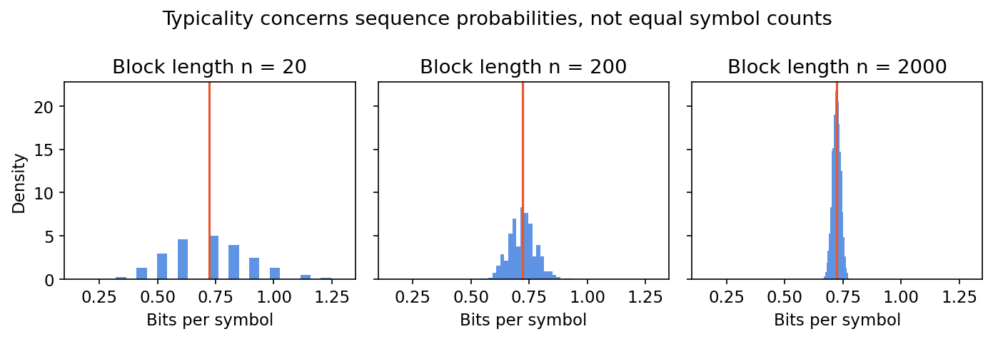
Code: exact typical probability and finite counts
The first complete example uses a binomial count distribution to sum typical-set probability exactly up to floating-point arithmetic. A separate small enumeration checks the cardinality bound.
Code · Python · 25 lines
import itertools
import numpy as np
from scipy.stats import binom

p, epsilon = 0.2, 0.1
entropy = -p * np.log2(p) - (1 - p) * np.log2(1 - p)
for n in [20, 200, 2000]:
    k = np.arange(n + 1)
    per_symbol = -(k / n) * np.log2(p) - (1 - k / n) * np.log2(1 - p)
    typical = np.abs(per_symbol - entropy) <= epsilon
    probability = binom.pmf(k, n, p)[typical].sum()
    print("Length:", n, "typical probability:", probability)

n, epsilon = 10, 0.15
count, mass = 0, 0.0
for block in itertools.product([0, 1], repeat=n):
    k = sum(block)
    probability = p**k * (1 - p)**(n - k)
    surprise = -np.log2(probability) / n
    if abs(surprise - entropy) <= epsilon:
        count += 1
        mass += probability
assert count <= 2**(n * (entropy + epsilon))
assert count >= mass * 2**(n * (entropy - epsilon))
print("Small-block typical count / mass:", count, mass)
Small-block typical mass need not be close to one. “Asymptotic” is a statement about growing block length with a fixed tolerance, not permission to apply the large-block conclusion at any length.
Worked example: count strings, then add their probabilities
Use the small enumeration above: , and . A block with ones has average surprise bits per symbol, while source entropy is 0.721928. Only satisfies the tolerance. This determines membership before we count anything.
There are such strings. Each has probability , so the typical set has probability . In contrast, the single all-zero string has probability . It outranks each typical string individually, but carries less probability than the 45 strings together.
These calculations answer three separate questions: membership is decided by surprise tolerance, cardinality counts accepted strings, and mass sums their probabilities. A catalog of 45 strings needs six fixed-length index bits because five bits identify only 32 alternatives. Yet that catalog covers only about 30.2% of this short-block source. The length-10 catalog alone is therefore a poor almost-lossless code, despite its rate of six tenths of a bit per symbol.
The entropy bound does not fail. Its high-probability conclusion requires longer blocks at this fixed tolerance. Cardinality rounding and excluded probability are finite-block costs that the limiting argument does not erase from a short experiment.
For comparison, scoring the same blocks with a fair-bit model would give exactly one bit per symbol to every block. That model cannot distinguish the all-zero string from a two-one string by surprise. The underlying source has not changed; the scoring model has. A typical-set computation must always specify which of those distributions supplies the probabilities.
Empirical frequencies and combinatorial intuition
A block’s symbol frequencies define a group of many strings with the same source probability. Counting that group explains how individually unlikely strings can dominate collectively.
For a binary block with exactly ones, the number of arrangements and the total probability of that count are
Here counts strings, is the random number of ones, is the binomial coefficient, and is the source probability of one. Every arrangement with that count has the same probability, but the number of arrangements varies dramatically.
At the extremes, there is just one all-zero string and one all-one string. Near the center, there are many arrangements. For a biased source, the probability assigned to each arrangement and the number of arrangements pull in different directions; their product peaks near the source’s expected count.
This viewpoint also clarifies why empirical-frequency typicality and surprise typicality are different. Under a fair binary source, every length- string has probability and average surprise exactly one bit. Therefore every possible string is weakly typical for any positive tolerance, including all zeros.
The probability of observing an all-zero string still tends to zero. A frequency-based typical set can exclude it by requiring the fraction of ones to stay near one half. Its probability also tends to one, but it has a stricter membership rule.
Neither definition is “wrong.” Each is useful for a different proof. A probability-scale statement may need only weak typicality; a construction that matches empirical conditional distributions may require stronger frequency control. Always check the definition actually used, especially when a proof moves from marginal source coding to joint input-output relationships.
A source-coding argument and its limitation
Number the typical blocks and send their catalog index. With enough symbols in each block, this uses close to entropy bits per symbol while failing only on a small excluded set.
Since the typical set has at most members, an index takes at most approximately bits, plus rounding and framing. A decoder uses the same catalog to reconstruct the selected block.
This is an almost-lossless fixed-length construction. It does not encode every possible block correctly. It can reserve one extra symbol for failure, but that flag does not reconstruct an atypical block. To make a truly lossless scheme, provide an escape representation with enough information to recover it.
A simple converse explains why rates well below entropy cannot cover most probability mass. Suppose a code can correctly represent at most blocks. Intersect those blocks with the typical set. Each typical block has probability at most , so their accepted mass is at most
Here is the fixed code rate in bits per source symbol. If , this typical accepted mass approaches zero. The omitted atypical mass also approaches zero, so the code cannot reconstruct the source with high probability.
This argument assumes the encoder-decoder pair has a limited number of distinct messages. It is a counting proof, not an efficient implementation. Enumerating a huge catalog is generally impractical. The next chapter studies prefix coding, probability coding and adaptive models that turn theoretical rates into computable procedures.
Add an escape branch to make the catalog lossless
A catalog that sometimes fails can be turned into a code that reconstructs every allowed finite block. Send a one-bit branch flag. If the block is typical, send its fixed-length catalog index. Otherwise, send an uncompressed representation of the block using a fixed number of bits per symbol.
Let and for a nonempty typical set. The expected length satisfies
Here is total block length in bits, is the fixed raw symbol width, the typical index width, the typical probability, and retain their earlier meanings. The equality counts the flag and the two branches; the inequality uses typical-set cardinality and upward integer rounding.
The decoder reads the flag first, so it knows which fixed branch length to read. The typical branch returns a shared catalog entry; the escape branch reconstructs the raw symbols. No block is silently dropped. If a small finite block has an empty typical set, use only the raw branch until a usable catalog exists.
For fixed , AEP gives , making the escape contribution vanish per symbol. The flag and rounding costs also vanish as grows. Then the expected rate approaches no more than . Choosing smaller tolerance after establishing sufficiently long blocks brings the rate arbitrarily close to entropy.
The construction reveals the difference between fixed-rate almost-lossless and variable-length fully lossless coding. The escape branch can be long on rare blocks, so the latter conclusion concerns expected length, not a short bound for every block. It also assumes encoder and decoder share the catalog and source model. This is a proof of attainable rates; explicit enumeration is generally too expensive to be a practical compression algorithm.
Finite-block concentration depends on the source
Long blocks are useful, but how long is enough depends on the source and the tolerance. Rare symbols can produce large surprise fluctuations.
For independent symbols with finite surprise variance,
Here is the source surprise variance and denotes variance. This follows from adding independent variances and dividing by . A general variance bound gives
Here is the same surprise tolerance as before. The bound can be loose, but it makes the dependence explicit. Very small probabilities can increase surprise variance, and demanding a narrow tolerance increases the required block length.
An empirical standard deviation across blocks is useful, but it is not a universal finite-block coding guarantee. Dependence changes the variance calculation; rare events may be missed by a small simulation; model mismatch changes the center of concentration.
If a source is scored by model , independent block average surprise converges to under integrability conditions, not to . The difference is relative entropy. Typical under the model and typical under the actual source are separate questions.
Entropy rates account for dependence
Neighboring symbols often help predict one another. The information required per symbol over a long sequence can therefore be smaller than the entropy of a single marginal symbol.
For a stochastic process , define its entropy rate when the limit exists:
Here is the average new uncertainty per symbol and is block length. This definition concerns block entropy, not a fitted model’s loss on one realized sequence.
The chain rule gives
Here is the preceding history, with empty history at . Dependence makes these conditional terms different from marginal entropy.
A process is stationary when shifting all time indices leaves every finite joint distribution unchanged. This is stronger than a constant mean or covariance. Under finite-alphabet stationarity, the conditional entropy given a longer past is nonincreasing and bounded below by zero, so its limit exists. The block-average entropy has the same limit.
The equality of these limits comes from averaging a convergent conditional-entropy sequence. Stationarity permits moving a fixed-length history to a common time index, where adding more past information reduces conditional entropy.
Independent identically distributed sources are a special case: each conditional entropy equals . A dependent stationary source may have the same marginal distribution at every time while requiring much less new information per step.
Markov sources provide an explicit calculation
A first-order Markov model needs only the current state to predict the next. Its long-run uncertainty averages the uncertainty in each transition row.
Let a finite Markov source have transition matrix :
Here and index source states, is time, is a transition probability, and is a stationary state distribution. Each row of sums to one; is nonnegative and sums to one.
If the process starts in , stationarity and the Markov property give
The inner sum is the entropy of transition row ; the outer sum weights rows by stationary occupancy. The finite block entropy is
Here is the entropy of the initial state. The chain rule contributes one initial term and identical transition terms.
For a symmetric binary source that flips with probability , the stationary distribution is uniform. Its marginal entropy is one bit, while its entropy rate is . With , most next symbols repeat the current symbol, reducing fresh uncertainty.
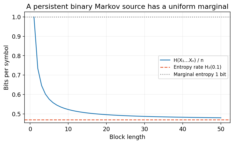
Code: predictability without changing the marginal
This standalone experiment generates stationary binary Markov blocks using independent flip events. It compares observed average surprise with the exact block-entropy formula.
Code · Python · 18 lines
import numpy as np

rng = np.random.default_rng(32)
a = 0.1
rate = -a * np.log2(a) - (1 - a) * np.log2(1 - a)
for n in [64, 256, 1024]:
    initial = rng.integers(2, size=1000)
    flips = rng.binomial(1, a, size=(1000, n - 1))
    states = np.column_stack([
        initial, initial[:, None] ^ np.bitwise_xor.accumulate(flips, axis=1)])
    surprise = 1 + (-flips * np.log2(a) - (1 - flips) * np.log2(1 - a)).sum(axis=1)
    expectation = (1 + (n - 1) * rate) / n
    print("Length:", n, "one-frequency:", states.mean(),
          "mean surprise rate:", surprise.mean() / n,
          "exact entropy per symbol:", expectation)
    assert abs(states.mean() - 0.5) < 0.08
    assert abs(surprise.mean() / n - expectation) < 0.02
print("Entropy rate:", rate, "marginal entropy:", 1.0)
The initial state is sampled uniformly, which makes this source stationary. Starting every block at zero changes finite-block distributions; the asymptotic rate can still agree under suitable transition assumptions, but the exact initial-entropy term changes.
Why a fair marginal can still be cheap to predict
For the symmetric Markov example with flip probability , the first bit costs one bit of uncertainty. Each later bit contributes bits. At length ten, the block entropy is bits, or 0.522096 bits per symbol. Ten independent fair bits would instead have ten bits of block entropy.
A useful representation is the initial bit followed by nine flip indicators. This mapping is invertible: starting from the first bit, exclusive-or each flip indicator to recover the next state. It makes the dependence visible without throwing away any source information. The indicators are biased independent bits under this particular model, so their distribution is easier to code than ten marginal fair states.
The long-run rate approaches 0.468996 because the one-bit initialization cost is divided by an increasing block length. Predictability comes from the transition relationship, even though every time position is marginally fair. An image histogram similarly cannot reveal all gains available from predicting pixels using their neighbors.
Hidden states and the choice of observation
A transition model may describe an internal state while the receiver sees only a noisy measurement. The observed sequence then has its own prediction problem.
Suppose is a finite hidden Markov state and an emitted observation. A model may factor a block as
Here is a state sequence, an observation sequence, and the factors describe transitions and emissions. Summing over hidden sequences gives the observed likelihood .
The entropy rate of is generally not just the stationary average of emission-row entropies. Past observations help infer the hidden state, and residual state uncertainty affects prediction. The relevant terms are , not only .
This is a useful warning for vision: a model of object dynamics and a model of camera measurements refer to different random processes. More sensor noise may increase observation entropy while decreasing useful information about the scene. Rate calculations must state which process is being described.
Ergodicity matters for a common typical value
Stationarity says distributions do not drift with time. It does not guarantee that one long realization explores all parts of a mixed population.
Under appropriate stationary ergodic finite-source assumptions, the long-block normalized surprise converges to a single entropy-rate value. Ergodicity rules out a persistent hidden choice that divides the process into separately behaving stationary components.
Consider choosing a component once: with probability one half, produce zeros forever; with probability one half, produce independent fair bits. Each component is stationary, and the mixture is stationary.
Conditional block entropy is . The identity
uses component label , block and mutual information . Since , the block-average entropy tends to one half bit.
Nevertheless, a realized sequence from the deterministic component has normalized surprise approaching zero; one from the fair component usually has normalized surprise approaching one. There is no single common value near one half for most realizations. An entropy-rate limit alone does not justify an ergodic AEP conclusion.
Code: a stationary nonergodic counterexample
This complete example computes the mixture block probability analytically from the number of ones. It avoids exponentiating a very small fair-block probability before taking its logarithm.
Code · Python · 14 lines
import numpy as np

rng = np.random.default_rng(33)
for n in [128, 1024]:
    component = rng.integers(2, size=2000)
    counts = rng.binomial(n, 0.5, size=2000) * component
    # A nonzero sequence can only come from the fair component:
    # its probability is 0.5 * 2**(-n), so surprise is n + 1.
    all_zero_surprise = -np.log2(0.5 + 0.5 * np.exp2(-float(n)))
    per_symbol = np.where(counts == 0, all_zero_surprise, n + 1) / n
    print("Length:", n, "deterministic mean:", per_symbol[component == 0].mean(),
          "fair mean:", per_symbol[component == 1].mean(),
          "fraction within 0.1 of 0.5:", np.mean(abs(per_symbol - 0.5) <= 0.1))
    assert np.mean(abs(per_symbol - 0.5) <= 0.1) == 0
This example is a model of persistent heterogeneity, not time drift. A dataset containing different source types can require conditional models or explicit mixtures rather than assuming one long recording represents the whole population.
Joint and conditional typicality
Two individually ordinary sequences can form an extraordinary pair. Communication proofs need the relationship between input and output, not only separate histograms.
For independent draws of pairs from joint mass function , consider the joint and conditional average surprises:
Here arrows mean convergence in probability under the specified independent-pair model. and are paired blocks; dependence within each pair is allowed.
A jointly typical pair is checked against the joint source relationship. Marginal typicality alone does not ensure this. If is a noisy copy of , two unrelated fair-bit sequences can each have typical marginal counts but the wrong mismatch frequency.
The per-block information density is
Here measures evidence for the joint pair relative to an independent pair model. Under independent paired sampling, its normalized average approaches when integrable.
This connects to channel decoding: a receiver looks for codewords whose relationship to the received block is consistent with the channel. It also connects to matching and representation learning, where positive pairs must be defined carefully. A negative pair drawn from the wrong population changes the reference distribution.
Strong typicality for finite alphabets additionally constrains empirical frequencies of each symbol or pair, respecting impossible events. Weak typicality constrains average log-probability. Neither notion should be silently substituted for the other in a proof whose assumptions use one specific definition.
Modern view
The distinction between average surprise and meaningful output is particularly relevant to modern probability models. Long contexts and learned predictors can model dependence beyond a fixed Markov order, but their loss is still scored under a particular observation and tokenization model.
El Gamal’s 2026 proposed learning chapter [3] gives a current divergence-based bridge to predictive and generative models. It is a draft supplement, not a published third edition. Our inference from the source-coding viewpoint is that sequence likelihood should always be reported with its prediction target, units and conditioning context.
Huang and Wu’s 2024 review [4] surveys learned image compression through the distinction between coding for human reconstruction and coding for machine analysis. Its taxonomy highlights that a useful compressed representation depends on the consumer. Entropy rate supplies a source-description limit, but it does not alone specify a task’s acceptable distortion.
Three practical questions remain open in many applications: how quickly asymptotic behavior becomes useful at actual block lengths; whether a fitted source model remains valid across populations; and how dependencies created by sampling, tokenization and preprocessing affect estimated rates.
Finite evaluation should compare independent blocks or acquisition groups and retain atypical cases. Reporting only average surprise can hide a rare source component with a much higher rate. Measuring likelihood under one model cannot establish that all source components share the same typical set.
The next chapter makes the bridge concrete: a coder must define its probability model, update rules, termination convention and treatment of unexpected symbols. A rate theorem guides those choices; a round-trip test checks whether the actual implementation reconstructs the intended data.
Key takeaways
- AEP concentrates normalized block surprise under stated source assumptions.
- Typical-set probability and cardinality are different quantities with different bounds.
- Most-probable individual blocks need not carry most collective probability mass.
- Typical catalogs explain almost-lossless coding limits, not efficient implementations.
- Entropy rate measures new uncertainty after dependence is exploited.
- Stationarity does not guarantee ergodicity or a common realized surprise rate.
- Joint typicality checks relationships that marginal typicality can miss.
- Finite-block behavior, source mismatch and heterogeneity must accompany asymptotic claims.
Exercises
- For a Bernoulli source with , calculate the all-zero block surprise rate and source entropy. Choose a tolerance that excludes all-zero blocks for every length.
Hint
Compare with .
- Repeat exact typical-mass computation at tolerances , and . Explain why smaller tolerance can require much longer blocks.
Hint
The average-surprise window narrows.
- Derive the typical-set lower and upper cardinality bounds using separate and . Identify which individual-probability bound is used in each step.
Hint
Bound a sum by count times the largest or smallest allowed block probability.
- A binary Markov chain has transition matrix . Find its stationary distribution, marginal entropy and entropy rate.
Hint
Solve and weight transition-row entropies.
- In the nonergodic mixture example, change the component probabilities to one quarter deterministic and three quarters fair. Find the block entropy-rate limit and realized surprise-rate limits.
Hint
The persistent component still prevents one common realized value.
- Construct two marginally typical fair-bit sequences that are not jointly typical under a 10% flip channel. Explain why separate symbol counts fail to detect the mismatch.
Hint
Use a pair with too many or too few disagreements.
References
- T. M. Cover and J. A. Thomas, Elements of Information Theory, 2nd ed., Wiley, 2006, Chapters 3–4. Publisher book and contents.
- T. Weissman, “Asymptotic Equipartition Property,” Stanford EE276 Lecture 3 notes, 2024. Primary lecture notes.
- A. El Gamal, “Information Theory and Statistical Learning,” proposed textbook chapter, arXiv preprint, 2026. Draft and publication status.
- C.-H. Huang and J.-L. Wu, “Unveiling the Future of Human and Machine Coding: A Survey of End-to-End Learned Image Compression,” Entropy, 26(5), 357, 2024. Published review.
Check your understanding
This tutorial has 6 exercises. Can you solve them without opening the hints?
Go to the exercises ↑Next IT 03 · Lossless Coding and Universal Compression · 18 min