IT 04 · Channel Capacity and Reliable Communication
Needs: IT 03 · Lossless Coding and Universal Compression
Navigate: this page and this track: Navigate: this page and this track
On this page
- What you’ll learn1 min
- The big picture1 min
- Define the channel before its capacity1 min
- Rate and reliability are operational quantities1 min
- A binary symmetric channel1 min
- A binary erasure channel1 min
- Asymmetric channels need asymmetric signaling1 min
- Why rates below capacity are achievable1 min
- Fano’s inequality limits what a receiver can infer2 min
- Computing capacity with Blahut–Arimoto2 min
- A repetition experiment shows the finite-block tradeoff1 min
- Resource constraints and different channel assumptions1 min
- Estimating a channel is a separate experiment1 min
- How source information meets channel information1 min
- Modern view1 min
- Key takeaways1 min
- Exercises1 min
- References
Information Theory
Explore this chapter 1 interactive experiment
Separate source uncertainty, transmitted information and channel capacity.
What you’ll learn
- Define a discrete memoryless channel and distinguish messages from channel symbols.
- Derive capacities of binary symmetric and binary erasure channels.
- Explain random-code achievability through joint typicality and packing.
- Use Fano’s inequality to derive a converse bound on reliable rate.
- Compute capacity and a diagnostic optimality gap with Blahut–Arimoto.
- Separate asymptotic limits from finite-block reliability and task-based communication.
The big picture
A noisy channel does not have to reproduce every transmitted symbol correctly for a receiver to recover the message. A code represents each message by a longer structured sequence. The receiver compares the noisy observation with the possible sequences and decides which message was sent.
Source coding removes predictable redundancy; channel coding adds useful redundancy. These are different objectives. Repeating a bit is an elementary channel code, but not necessarily a good use of the channel. The central question is how many distinct messages can be communicated per channel use while their reconstruction error tends to zero.
The main reading is Cover and Thomas’s Chapter 7; the book’s computational discussion connects capacity optimization with the Blahut–Arimoto method [1]. Stanford’s communication and converse notes [2,3] give primary derivations. We develop the theorem’s assumptions and a numerical experiment, then explain why practical short messages need additional evaluation.
Define the channel before its capacity
A channel specifies how an input symbol is randomly transformed into an output symbol. The source distribution and the channel transformation are separate objects.
For finite input alphabet and output alphabet , a discrete memoryless channel is a row-stochastic matrix
Here index symbols, and each row sums to one. The blocks have length , and indexes a use. The factorization defines memorylessness and a time-invariant transition law.
Memorylessness concerns outputs conditioned on the entire input block. A code’s input symbols may be dependent, because all are determined by one message. Their unconditional outputs can consequently be dependent too. Assuming independent inputs when proving a converse would restrict the permitted codes unnecessarily.
The sender chooses an input distribution for a single-letter calculation. It induces output probability
Here is the output marginal. The channel stays fixed as changes. Altering the propagation law, receiver observations, resource constraints or available feedback defines a different communication problem.
Rows that are identical cannot distinguish their corresponding inputs. Distinct rows may be easier or harder to distinguish depending on overlap. Output alphabet size gives a crude upper bound on information, but the transition probabilities determine the actual usable distinction.
Rate and reliability are operational quantities
A communication rate counts message information divided by channel uses. Reliability refers to recovering the whole message, not simply making most channel symbols correct.
Let a message be uniform over alternatives. A length- code maps it to and estimates from received . Define
Here is codebook size, is bits per channel use, and is average message-error probability under the specified uniform message and channel. These are different from symbol-error rate.
A rate is achievable if there is a sequence of codes with asymptotic rates at least and message error tending to zero. Capacity is the supremum of achievable rates:
Here ranges over all input probability distributions on the finite alphabet and is mutual information under . The second equality is the channel-coding theorem for the stated finite memoryless channel [1,2].
The theorem describes rates strictly below capacity in its standard achievability statement. It does not promise zero error at finite length or provide a fast decoder. Capacity also differs from zero-error capacity, which demands that allowed output sets never confuse messages. A channel can have positive ordinary capacity while every finite block still has a nonzero confusion probability.
The average-error formulation has a uniform message assumption. Maximum error across messages is another operational criterion; standard finite memoryless results connect the capacity formulations by expurgating poor codewords with negligible asymptotic rate loss. At finite length their reliability statistics can differ.
A binary symmetric channel
Each bit is independently flipped with the same probability. A fair input makes full use of the two output alternatives.
For crossover probability , the binary symmetric channel has
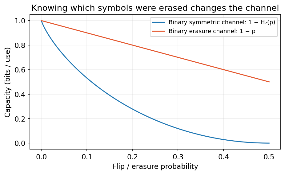
Here is the flip probability, is binary entropy, and capacity is bits per use. Conditional output entropy is for either input. Since , mutual information is at most ; a fair input attains the bound.
At , one use conveys one bit without noise. At , output is independent of input and capacity is zero. At , every bit flips deterministically, so the receiver can invert it and capacity is again one. Noise severity is therefore not simply the raw flip fraction across the entire interval.
The figure restricts crossover probability to zero through one half, where the ordinary interpretation of increasing uncertainty is natural. The complementary branch follows by relabeling outputs.
A binary erasure channel
The receiver either sees the correct bit or a visible “missing” marker. Knowing which observations are missing is useful information.
A binary erasure channel with erasure probability has outputs zero, one and an erasure symbol:
Here rows correspond to input zero and one, while columns correspond to the two correct symbols and the erasure. The erasure event is independent of the input.
Conditioned on a nonerased output, the input is known. Conditioned on erasure, its uncertainty remains . Therefore and a fair input attains bits per use.
The same numerical event probability produces different capacities for flips and visible erasures. An erasure tells the receiver where information is missing; an unmarked flip can actively suggest the wrong alternative. The distinction follows from their different output laws, not a universal ranking for every physical communication system.
Asymmetric channels need asymmetric signaling
When one input is more reliable than another, a uniform input distribution need not be best. Capacity optimizes how often inputs are used.
Consider a Z channel where zero arrives correctly and one becomes zero with probability :
Here is the one-to-zero transition probability, and is the scalar input parameter. Output one has probability ; conditional output entropy is .
The first term rewards varied outputs, while the second accounts for noise paid when using input one. Their tradeoff can place the maximum away from . Transmitting only the reliable zero is not useful either: a constant input conveys no message information.
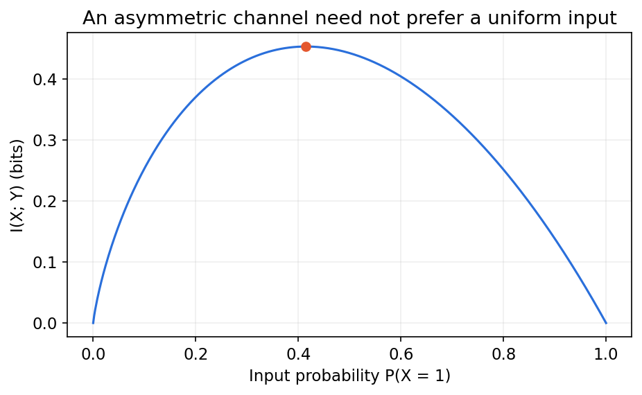
Mutual information is concave as a function of the input distribution because output entropy is concave and conditional output entropy is linear. Concavity makes numerical optimization tractable. Flat maxima can still exist when different inputs are redundant, so an optimal input distribution need not be unique.
Why rates below capacity are achievable
Choose many long codewords that look like valid source blocks. A received block usually matches its true codeword’s channel relationship, while it rarely matches an unrelated codeword.
Fix an input distribution and generate approximately codewords independently from . A jointly typical decoder looks for one codeword consistent with the received output under the joint law [1].
There are two main errors: the true input-output pair fails its typicality test, or another codeword passes. The first probability vanishes by the joint AEP. An independent competing codeword has a joint-typicality probability at an exponential scale near .
A union bound over the competing codewords gives the schematic scale
Here is the probability of a competing typical codeword, absorbs the typicality tolerances, and suppresses finite prefactors and detailed bounds. This is proof intuition, not an exact finite-length performance formula.
When , the competing-error bound vanishes. Choosing a maximizing input and sufficiently small tolerance gives rates below capacity. A small average error over random codebooks implies at least one deterministic codebook has small error.
The argument does not require transmitting the random seed for each message. The codebook is fixed and known to both endpoints before communication. If a practical system chooses or sends new codebooks, that setup protocol must be counted separately.
Random coding proves existence. Searching every codeword in an exponentially large codebook is generally infeasible, and typicality is not a direct recipe for a deployed decoder. A capacity theorem identifies a target; practical structured codes solve the additional complexity problem.
Fano’s inequality limits what a receiver can infer
If the receiver frequently guesses wrong, uncertainty remains about the message. Conversely, a small error probability means little conditional message uncertainty remains.
With possible messages and any estimate based on ,
Here is the true message, the received block, , and binary entropy. This is Fano’s inequality [1,3].
To see the logic, introduce an error indicator. Describing whether an error happened costs at most its binary entropy. If no error happened, the estimate identifies the message. If an error happened, at most alternatives remain. Averaging yields the first bound.
For a uniform message, . Data processing and channel memorylessness bound
Here is the transmitted codeword. The middle inequality allows dependent code symbols: output entropy is at most the sum of marginal output entropies, while conditional output entropy separates under the memoryless channel.
Combining the two bounds gives
Here and the lower bound is meaningful only when its right-hand side is positive. A fixed rate strictly above capacity cannot have vanishing error.
This elementary converse establishes a positive error floor above capacity, not by itself convergence of error to one. Strong-converse statements require an additional theorem and assumptions. It is good practice to state exactly what the displayed inequality proves.
Worked rate, error and source-budget calculations
For crossover probability , the BSC capacity is bits per use. The BEC at the same erasure probability has capacity 0.9. This is a difference between observation models: the BEC reveals which symbols were lost.
A length-100 code at rate 0.8 contains possible messages. Substitute the BSC capacity into the elementary converse:
Here is average whole-message error, 100 is the number of channel uses and 0.8 the message bits per use. The rounded capacity in the substitution retains more digits than the reported answer. This code cannot achieve a 1% message-error target under the stated channel, whatever its decoder. The bound does not determine the exact error of any specific code.
At rate 0.5 the same displayed lower bound is negative, so it provides only the trivial bound zero. That is consistent with asymptotic achievability below capacity, but it does not demonstrate that length 100 already provides the desired reliability. The two questions are answered by different evidence: a theorem for growing block length and a finite-code calculation or experiment.
Now take an independent binary source with probability 0.2 of one. Its entropy is 0.721928 bits per source symbol. Transporting it almost losslessly over this BSC requires more than channel uses per source symbol in the asymptotic separation setting. One use is insufficient; two uses leave a rate margin. A raw-source representation would require one bit per source symbol before channel coding, illustrating why exploiting source bias and protecting against noise are separate design steps.
The bandwidth ratio need not be an integer. Over a long block, a rational or approximate ratio is implemented by allocating the corresponding total number of channel uses. Latency and finite-block overhead remain additional constraints.
Computing capacity with Blahut–Arimoto
Start with an input mixture, examine how distinguishable each channel row is from its output mixture, then move probability toward informative rows. Repeat until an upper and lower bound nearly meet.
For current positive input probabilities and induced , define row divergences in natural units:
Here is the divergence between channel row and the current output distribution, is the natural logarithm, and indexes inputs. The denominator uses the same current distribution; the update does not replace it with a uniform prior. Values in nats convert to bits by division by .
For the current distribution, the lower and upper bounds are
Here is current mutual information and is a dual-style bound obtained by using the current output mixture as a candidate reference distribution. The gap gives a useful numerical stopping criterion.
This unconstrained algorithm applies to a fixed finite channel. An input-cost constraint requires a modified optimization; one cannot compute unconstrained capacity and claim compliance with a power or symbol-use budget afterward.
Why the numerical upper bound is valid
A stopping gap is useful only if its endpoints actually bracket the optimum. Fix the current output mixture , then consider any candidate input distribution , whose output mixture is . Expanding the logarithmic ratios gives
Here is channel row , its candidate usage probability, the fixed reference output distribution, the candidate output marginal and mutual information under . All quantities in this identity use natural logarithms.
The final divergence is nonnegative, so the candidate information is no larger than the weighted sum on the left. That sum is no larger than its largest row divergence. Because this holds for every candidate , the current maximum row divergence upper-bounds capacity. The current input’s own information is achievable in the single-letter optimization and supplies the lower bound.
At an optimum, inputs assigned positive probability have equal informative row divergences, while unused inputs cannot offer a larger marginal gain. The updates redistribute probability toward rows with greater current divergence until these conditions nearly balance. The gap therefore measures how much improvement could remain for this matrix, rather than merely how small the latest parameter update was.
Code: validate analytic capacities and optimize the Z channel
The complete implementation removes output columns that are impossible for all inputs, masks zero row entries and uses a stable logarithmic normalization. It returns the current input distribution associated with its lower-bound rate.
Code · Python · 43 lines
import numpy as np
from scipy.special import logsumexp
from scipy.optimize import minimize_scalar

def binary_entropy(p):
    if p == 0 or p == 1:
        return 0.0
    return -p * np.log2(p) - (1 - p) * np.log2(1 - p)

def capacity(W, tolerance=1e-10, maximum=20000):
    W = np.asarray(W, dtype=float)
    assert W.ndim == 2 and np.all(W >= 0)
    assert np.allclose(W.sum(axis=1), 1)
    W = W[:, W.sum(axis=0) > 0]
    q = np.full(W.shape[0], 1 / W.shape[0])
    positive = W > 0
    for iteration in range(maximum):
        r = q @ W
        ratio = np.zeros_like(W)
        np.log(np.divide(W, r, out=np.ones_like(W), where=positive),
               out=ratio, where=positive)
        d = (W * ratio).sum(axis=1)
        lower, upper = q @ d / np.log(2), d.max() / np.log(2)
        if upper - lower < tolerance:
            return lower, q, upper - lower, iteration + 1
        log_q = np.log(q) + d
        q = np.exp(log_q - logsumexp(log_q))
    raise RuntimeError("Capacity iteration did not meet the requested gap")

e = 0.1
bsc = np.array([[1-e, e], [e, 1-e]])
bec = np.array([[1-e, 0, e], [0, 1-e, e]])
for W, analytic in [(bsc, 1-binary_entropy(e)), (bec, 1-e)]:
    value, q, gap, steps = capacity(W)
    print("Capacity / analytic / input / gap:", value, analytic, q, gap)
    assert abs(value - analytic) < 1e-8
a = 0.35
z = np.array([[1, 0], [a, 1-a]])
value, q, gap, steps = capacity(z)
objective = lambda p: binary_entropy(p*(1-a)) - p*binary_entropy(a)
reference = minimize_scalar(lambda p: -objective(p), bounds=(0, 1), method="bounded")
assert abs(value + reference.fun) < 1e-8
print("Z capacity / P(input one) / gap / iterations:", value, q[1], gap, steps)
Agreement with analytic binary cases checks units and orientation. Agreement with independent scalar optimization checks the asymmetric case. These are meaningful tests because they would catch using column-stochastic probabilities, omitting the current factor or mixing natural and base-two logarithms.
Nearly redundant inputs and extreme probabilities can converge slowly or cause floating-point underflow. A small reported gap is a numerical certificate for this finite matrix within computational precision, not evidence that the matrix accurately describes a real channel.
A repetition experiment shows the finite-block tradeoff
Repeating one bit helps majority decoding, but consumes more uses per message bit. Higher reliability does not automatically mean a capacity-efficient code.
Repeating a bit times through an independent BSC and majority decoding, with odd , gives
Here is the number of flipped copies, the crossover probability, the one-bit message error, and the code rate. This is an exact finite-code calculation, not a capacity formula.
Code · Python · 12 lines
import numpy as np
from scipy.stats import binom

rng = np.random.default_rng(35)
e = 0.1
for copies in [1, 3, 5, 9]:
    noise = rng.binomial(1, e, size=(50000, copies))
    observed_error = np.mean(noise.sum(axis=1) > copies // 2)
    exact_error = binom.sf(copies // 2, copies, e)
    print("Copies / rate / simulated error / exact error:",
          copies, 1 / copies, observed_error, exact_error)
    assert abs(observed_error - exact_error) < 0.005
We may assume a zero message bit when simulating this symmetric code, because either transmitted bit has the same error probability. More copies reduce error for this one-bit problem while driving rate toward zero. Capacity instead permits codebooks carrying a growing number of bits at a positive asymptotic rate.
A finite evaluation should specify block length, rate, message-error criterion, channel parameters and decoding rule. Reporting only a capacity number does not characterize a short code’s latency, complexity or reliability.
Resource constraints and different channel assumptions
A capacity calculation answers one precisely specified question. Changing a transmitter’s budget, adding memory or providing a different observation changes that question.
If input has nonnegative cost and the average budget per use is , the constrained single-letter problem is
Here is the input-use cost, the allowed mean, and a probability distribution satisfying it. The channel remains the same finite memoryless matrix. This formula concerns an average cost convention; a strict peak constraint on each symbol defines a different feasible set.
For an asymmetric binary channel, a constraint on the frequency of input one can exclude the unconstrained maximizing distribution. The result should be a capacity–cost function rather than one unconstrained number with a power label attached.
Likewise, throughput in bits per second requires a specified number of channel uses per second. Bits per use are not automatically bits per sample, pixel or token. When comparing modulation or representation choices, state how each choice changes the use count and available resources.
Feedback lets an encoder observe earlier channel outputs before choosing the next input. For the ordinary memoryless point-to-point model, noiseless causal feedback does not increase the asymptotic capacity [1,3]. It can still change finite-code design, stopping rules and achievable error behavior. This result should not be transferred without checking to channels with memory or multiple users.
A channel with a persistent hidden noise state may produce bursts rather than independent flips. A single transition matrix estimated by pooling all uses hides that dependence. The capacity proof above uses the conditional product law and cannot simply treat those bursts as independent draws with an average flip probability.
These distinctions also arise when a receiver supplies side information. If the side information reveals an erasure position, a noise state or part of the original message, it changes the receiver’s observation. Compare the entire observation model, rather than crediting a decoder for information that a baseline was denied.
Estimating a channel is a separate experiment
Numerical optimization can be exact for a wrong matrix. Before trusting the rate, determine whether the transition probabilities describe the operating conditions.
With labeled input–output observations, a simple row estimate is
Here counts observed input paired with output , ranges over outputs, and is an empirical channel matrix. Every input row needs observations. A zero empirical count does not prove an event impossible.
Finite samples create uncertainty in both the estimated capacity and the maximizing distribution. Repeating experiments across independent acquisitions can expose variability; conditioning on known operating regimes can reveal different channel laws. The optimizer’s gap measures computational convergence for one matrix, while experimental uncertainty concerns which matrix should be optimized.
Training and evaluation should also use separate observations when a decoder or input strategy is fitted from data. Selecting a favorable input distribution on the same tiny sample used to estimate its performance can produce an optimistic rate estimate.
A useful report therefore gives the sampling protocol, counts per input, operating conditions, empirical row probabilities, and held-out reconstruction results. Rare output events deserve explicit treatment because assigning them zero probability can distort both a decoder and an information estimate.
How source information meets channel information
A source coder packs useful uncertainty into bits; a channel coder carries those bits reliably. Their rates must be compared using the same source-to-channel use budget.
If a finite memoryless source has entropy bits per source symbol and channel uses are available per source symbol, the familiar asymptotic separation condition is
Here is a source symbol, is the use ratio and the point-to-point capacity. Under the standard long-block assumptions, source and channel coding can separately approach their limits with a margin [1].
The inequality does not specify a practical block size or require independent design to be optimal at finite latency. It also does not assert general source–channel separation for every network. Keeping its assumptions visible prevents the attractive formula from being applied to unrelated constraints.
For lossy reconstruction, the needed source rate becomes a rate–distortion function rather than full entropy. For continuous amplitudes, physical constraints determine channel capacity. These two extensions motivate the next chapters.
Modern view
Nguyen and colleagues’ 2025 published survey [4] organizes semantic communication into receiver-intention modeling, generative models, and deep joint source–channel coding. Its taxonomy distinguishes systems by what they aim to preserve and how transmitter and receiver coordinate, rather than treating every learned system as the same codec.
Those objectives can change the required reconstruction. A task receiver might need a class label rather than every original pixel. That can reduce required source information, but it does not increase the Shannon capacity of an unchanged channel under unchanged constraints.
Generative reconstruction similarly needs an explicit criterion. A plausible output can have a different relationship to the original than an exact decoded message. Evaluating task accuracy or perceptual distortion is legitimate when stated, but those quantities cannot replace message-error probability in a bit-reliability claim.
Our inference from the classical model is to keep three layers separate: what the source receiver needs, what the channel physically conveys, and how the code uses finite resources. Joint optimization can improve their practical match without invalidating any of the corresponding limits.
Open questions include robust performance when the channel law shifts, reliable operation at short block lengths, shared-model synchronization, and evaluation across different tasks and receiver knowledge. Survey results for one task or channel do not establish a universal semantic rate.
The next chapter changes alphabets from finite symbols to continuous amplitudes. It introduces differential entropy and power constraints before deriving Gaussian capacity; substituting a continuous density into a discrete entropy formula would miss essential unit dependence.
Key takeaways
- A memoryless channel factors outputs given inputs; code symbols need not be independent.
- Capacity is a reliable-message rate, equal to optimized mutual information under stated assumptions.
- Flips and marked erasures have different channel capacities.
- Asymmetric channels may favor nonuniform input probabilities.
- Random coding establishes existence through typicality and packing.
- Fano and data processing bound rates with vanishing message error.
- Blahut–Arimoto optimizes a finite channel and supplies a numerical gap.
- Finite reliability and semantic objectives require their own explicit evaluation.
Exercises
- Explain why a BSC with crossover probability 0.9 has the same capacity as one with probability 0.1. Describe the receiver’s output relabeling.
Hint
Invert every output.
- Derive the BEC mutual information for an arbitrary binary input probability rather than assuming a fair input.
Hint
Erasures leave the original input entropy.
- Change the Z-channel parameter to 0.1 and 0.7. Compare optimized input probabilities with one half and explain the competing entropy terms.
Hint
Optimize output entropy minus weighted row entropy.
- For a length-100 code of rate 0.8 through a BSC with crossover probability 0.1, calculate the elementary Fano lower bound on message error. State what it does and does not prove.
Hint
Use and keep a zero lower bound if negative.
- Duplicate a row in a channel matrix and rerun the capacity routine. Explain why the value is unchanged while an optimal input mixture may cease to be unique.
Hint
Identical rows produce identical conditional outputs.
- Compare repetition lengths 3 and 9 at equal total channel-use budgets. Explain why the smaller one-bit error cannot alone decide which system carries more reliably decoded information.
Hint
Count message bits as well as their errors.
References
- T. M. Cover and J. A. Thomas, Elements of Information Theory, 2nd ed., Wiley, 2006, Chapter 7 and the computational capacity/rate–distortion discussion. Publisher book and contents.
- T. Weissman, “Communication and Channel Capacity,” Stanford EE276 Lecture 7 notes, 2024. Primary lecture notes.
- T. Weissman, “Channel Coding Theorem: Converse Part,” Stanford EE276 Lecture 10 notes, 2024. Primary lecture notes.
- L. X. Nguyen, A. D. Raha, P. S. Aung, D. Niyato, Z. Han and C. S. Hong, “A Contemporary Survey on Semantic Communications: Theory of Mind, Generative AI, and Deep Joint Source-Channel Coding,” IEEE Communications Surveys & Tutorials, 2025, DOI: 10.1109/COMST.2025.3616973. Published-paper metadata and author version.
Check your understanding
This tutorial has 6 exercises. Can you solve them without opening the hints?
Go to the exercises ↑Next IT 05 · Differential Entropy and Gaussian Channels · 18 min