DL 01 · Deep Learning for Image Processing and Computer Vision

What you’ll learn

• How the classical three levels of image work (image processing, image analysis, computer vision) map onto the two families that deep learning actually uses: low-level and high-level vision tasks.
• Why the textbook pattern-recognition pipeline (sensor → features → classifier → evaluation) was replaced by end-to-end learning, and how it quietly came back as “pretrained backbone + light head”.
• How a convolutional layer is a bank of learned spatial filters, and how kernel size, stride, padding and pooling set the receptive field and the feature hierarchy.
• The design reasons behind the landmark CNNs (LeNet-5, AlexNet, VGG, GoogLeNet, ResNet) and the encoder–decoder (FCN, U-Net) used for dense prediction.
• How the Vision Transformer works, why it needs large-scale pretraining, and how Swin, ConvNeXt and self-supervised backbones (DINO, MAE, DINOv2/v3) answered it.
• A map of today’s tasks and representative models: classification, detection, segmentation (the SAM family), restoration and enhancement, generation (diffusion, latent diffusion, DiT) and vision–language models (CLIP, LLaVA).

The big picture

This tutorial is the entry point of the deep-learning track. It does not go deep into any one task. Instead it gives you the map: what kinds of image problems exist, which network designs solve them, and why those designs look the way they do. The later tutorials then zoom in on image classification, object detection, image restoration, low-light enhancement and object tracking.

Why it matters: almost every modern camera pipeline, medical-imaging product, driver-assistance system and photo app is built from the pieces in this tutorial. Knowing the map lets you pick a sensible starting point for a new problem, read papers critically, and understand which classical ideas from the Digital Image Processing series survive inside the networks (many do).

Three levels of image tasks

Plain version. “Image processing” in the broad sense covers three kinds of work. Some operations turn an image into a better image. Some pull out a particular part or property of the image. Some try to understand the image the way a person would.

Precise version. Following Gonzalez and Woods [2], we can sort image work into three levels by what goes in and what comes out.

Level	Input → output	Typical operations	Classical examples
Image processing (narrow sense; low level)	image → image	primitive, pixel- or neighborhood-wise steps	histogram equalization, filtering, Fourier transform (DIP 03, DIP 04)
Image analysis (mid level)	image → attributes or highlighted regions	segmentation, feature extraction, description, using prior knowledge	skin-color regions in a face image, vessel regions in an X-ray (DIP 10, DIP 12)
Computer vision (high level; understanding)	image → meaning	recognition, interpretation, decision	classification, “is there a pedestrian?” (DIP 13)

The boundaries are soft. Real systems mix all three. A vessel-segmentation tool, for instance, first denoises (low level), then extracts a vessel map (mid level), and may then flag a stenosis (high level). The levels describe kinds of computation, not separate departments.

How deep learning redraws the map

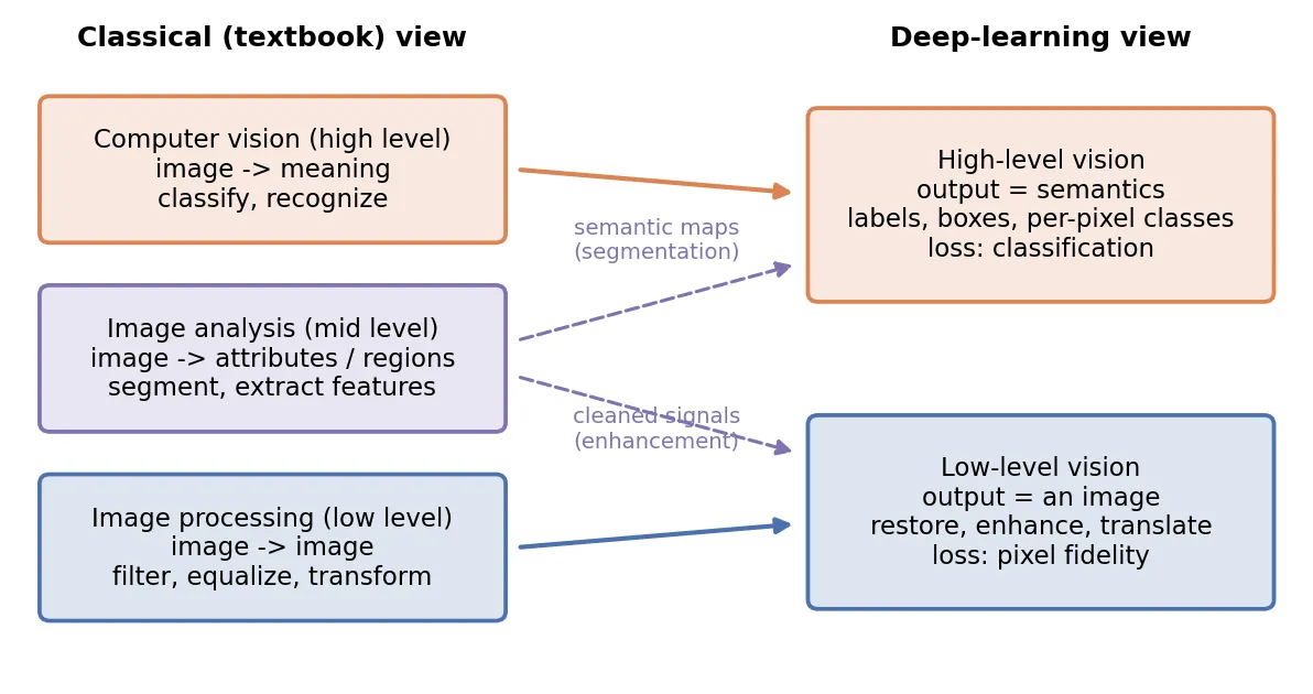
In deep-learning papers you will almost never see the word “mid-level”. The field splits tasks into just two families, according to the shape of the output [1]:

• Low-level vision: the output is an image of (roughly) the same size as the input, and the target is a pixel-accurate signal. Denoising, deblurring, super-resolution, dehazing, low-light enhancement, image-to-image translation.
• High-level vision: the output is a semantic description. A label, boxes with labels, or a label per pixel.

The old “image analysis” level is absorbed into one of the two. Segmentation produces a per-pixel map, so it looks like an image-to-image task. But its values are class labels that require recognition, so it is grouped with high-level vision. Edge or vessel enhancement that outputs a cleaner intensity image is grouped with low-level vision.

The reason for the split is practical. The two families differ in the loss (pixel regression versus classification), the architecture (full-resolution encoder–decoders versus downsampling backbones), the training data (pairs of degraded and clean images versus human labels) and the metrics (fidelity versus accuracy). Figure 1 shows the reorganization.

From the pattern-recognition pipeline to end-to-end learning

Plain version. Before deep learning, a recognition system was built like an assembly line: a camera, then a hand-designed step that measures useful properties, then a classifier that decides. Deep learning fuses the middle steps into one network that learns its own measurements.

Precise version. The classical pipeline [3] has four stages:

1. Sensor. Capture the pattern (camera, scanner, microscope).
2. Feature generation and selection. Compute a vector $\mathbf{x} = \phi(I) \in \mathbb{R}^d$ from image $I$, using a hand-designed map $\phi$ (moments, texture statistics, edge histograms, keypoint descriptors), then keep the most informative entries.
3. Classifier design. Learn a decision rule $\hat y = g(\mathbf{x}; \theta)$ with parameters $\theta$, for example a Bayes classifier, a nearest-neighbor rule or a support-vector machine.
4. System evaluation. Measure the error rate on held-out data and go back to step 2 or 3 if it is too high.

Only $\theta$ is learned. The feature map $\phi$ is fixed by an engineer, so the whole system is only as good as $\phi$. The chapter on feature extraction (DIP 12) shows how much ingenuity went into those maps.

End-to-end learning makes the feature map learnable too. A deep network computes

$$\hat y = g\big(\phi(I; \mathbf{w}); \theta\big),$$

where $\phi(\cdot\,; \mathbf{w})$ is a stack of layers with weights $\mathbf{w}$, $g(\cdot\,; \theta)$ is a small head, and both $\mathbf{w}$ and $\theta$ are fitted jointly by minimizing a loss $\mathcal{L}(\hat y, y)$ over labeled pairs $(I, y)$ with gradient descent and backpropagation. The input is raw pixels; nothing is hand-designed except the architecture and the loss.

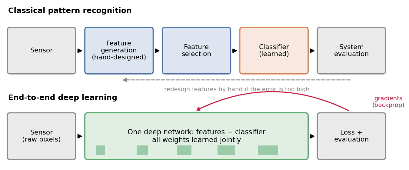
The functional split still exists inside a network: early layers behave like feature extractors and the last layers like a classifier. But in practice you usually cannot point at a layer and say “here the features end” [1]. Two consequences follow.

• Data replaces design. End-to-end systems need many labeled examples; the hand-designed $\phi$ encoded prior knowledge that the network must now learn from data.
• The split came back at a larger scale. Since about 2021 the standard recipe is a pretrained backbone (trained once, often without labels, on a huge dataset) plus a light task head trained on your small dataset. That is “feature extractor + classifier” again, except the feature extractor is learned rather than designed. We return to this in the section on self-supervised backbones.

Convolutional neural networks

Plain version. A convolutional layer slides a small window over the image and computes a weighted sum at every position, exactly like the spatial filters of DIP 03. The difference is that a CNN learns the weights of its filters, uses many filters at once, and stacks dozens of such layers with nonlinearities in between.

A convolutional layer is a bank of learned filters

Precise version. Let the input feature map be $X \in \mathbb{R}^{C_{\text{in}} \times H \times W}$ (channels, height, width). A convolutional layer with $C_{\text{out}}$ filters of size $k \times k$ computes

$$Y_{o}(x, y) = b_o + \sum_{c=1}^{C_{\text{in}}} \sum_{i=-r}^{r} \sum_{j=-r}^{r} W_{o,c}(i, j)\, X_c(x + i,\, y + j), \qquad o = 1, \dots, C_{\text{out}},$$

where $r = (k-1)/2$ for odd $k$, $W_{o,c}(i,j)$ is the weight of filter $o$ on input channel $c$ at offset $(i, j)$, and $b_o$ is a bias. Strictly this is a correlation (no kernel flip), as explained in the convolution tutorial; since the weights are learned, the flip makes no difference. An elementwise nonlinearity such as $\mathrm{ReLU}(z) = \max(0, z)$ follows. Without it, a stack of convolutions would collapse into one big linear filter [1].

Two properties make this layer the right tool for images:

• Local connectivity. Each output depends only on a $k \times k$ neighborhood, because nearby pixels are strongly related and distant ones much less so.
• Weight sharing. The same filter is used at every position. This makes the layer translation-equivariant (shift the input, and the output shifts the same way) and slashes the number of parameters.

The saving is huge. A fully connected layer from a $224 \times 224 \times 3$ image to 64 units needs $224 \cdot 224 \cdot 3 \cdot 64 + 64 \approx 9.6$ million parameters. A $3 \times 3$ convolution from 3 to 64 channels needs $3 \cdot 3 \cdot 3 \cdot 64 + 64 = 1{,}792$, and it produces 64 full-resolution feature maps instead of 64 numbers.

The code below sets the two filters of a PyTorch convolution by hand to Sobel kernels, which turns the layer into an edge detector. Training would instead set these numbers by gradient descent.

import torch, torch.nn as nn, torch.nn.functional as F
from skimage import data, img_as_float

x = torch.tensor(img_as_float(data.camera()), dtype=torch.float32)[None, None]  # (1, 1, 512, 512)
conv = nn.Conv2d(1, 2, kernel_size=3, padding=1, bias=False)
sobel_x = torch.tensor([[-1., 0., 1.], [-2., 0., 2.], [-1., 0., 1.]])
with torch.no_grad():
    conv.weight[0, 0] = sobel_x        # channel 0: responds to vertical edges
    conv.weight[1, 0] = sobel_x.T      # channel 1: responds to horizontal edges
    y = F.relu(conv(x))                # (1, 2, 512, 512): two feature maps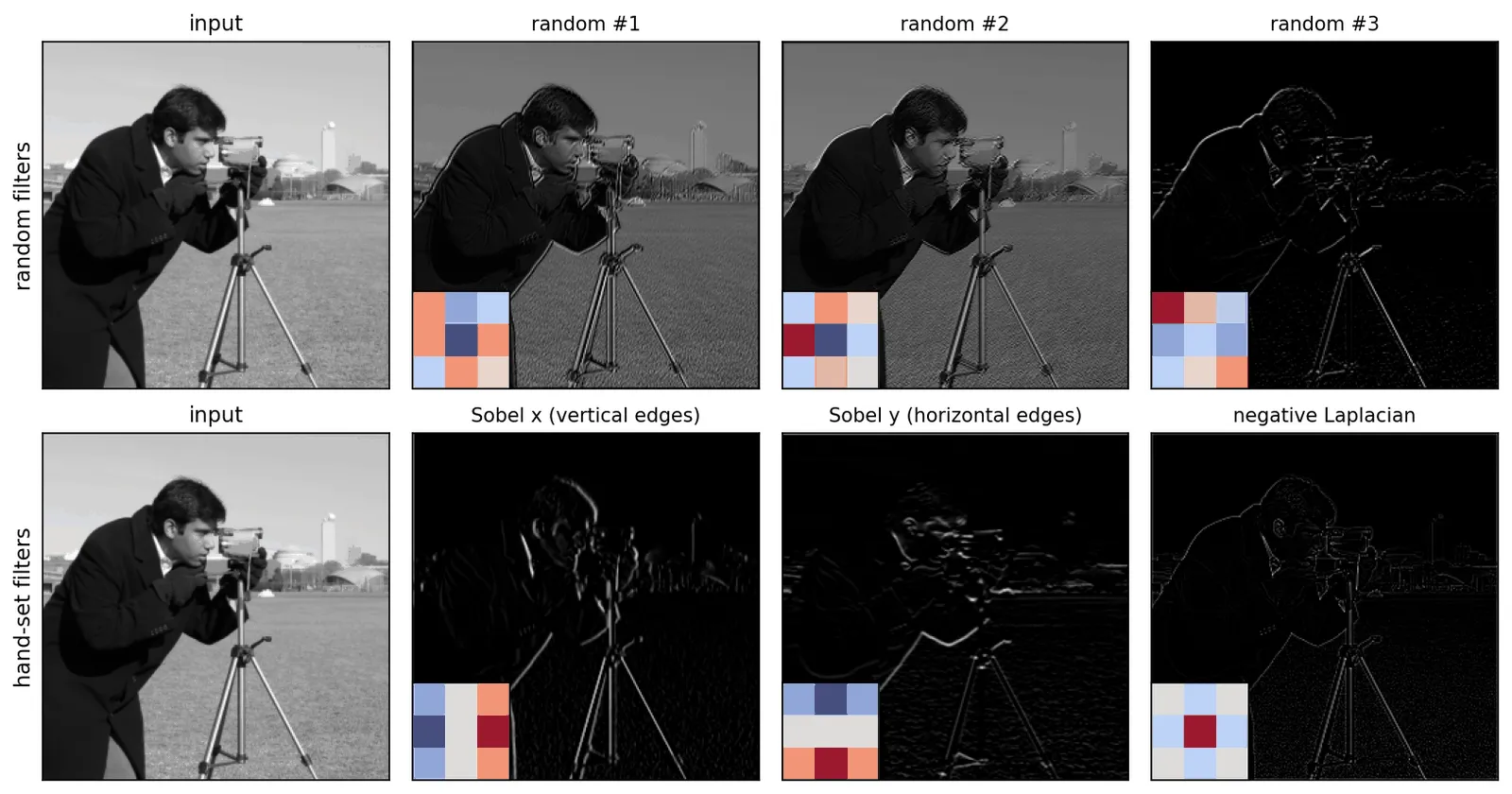

What do trained first-layer filters look like? We can train a tiny CNN on the 8×8 handwritten digits that ship with scikit-learn [36] in a few seconds on a CPU.

import torch, torch.nn as nn
from sklearn.datasets import load_digits
from sklearn.model_selection import train_test_split

torch.manual_seed(0)
X, y = load_digits(return_X_y=True)                    # 1,797 images of 8x8 pixels
X = torch.tensor(X / 16.0, dtype=torch.float32).reshape(-1, 1, 8, 8)
Xtr, Xte, ytr, yte = train_test_split(X, torch.tensor(y), test_size=0.25, random_state=0)

net = nn.Sequential(
    nn.Conv2d(1, 8, 3, padding=1), nn.ReLU(), nn.MaxPool2d(2),     # 8x8 -> 4x4
    nn.Conv2d(8, 16, 3, padding=1), nn.ReLU(), nn.MaxPool2d(2),    # 4x4 -> 2x2
    nn.Flatten(), nn.Linear(16 * 2 * 2, 10),
)
opt = torch.optim.Adam(net.parameters(), lr=1e-2)
for epoch in range(30):
    for i in range(0, len(Xtr), 64):
        loss = nn.functional.cross_entropy(net(Xtr[i:i + 64]), ytr[i:i + 64])
        opt.zero_grad(); loss.backward(); opt.step()
print((net(Xte).argmax(1) == yte).float().mean())       # about 0.97
filters = net[0].weight.detach()[:, 0]                   # (8, 3, 3) learned kernels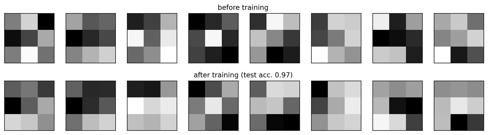

Stride, padding and output size

Plain version. Padding adds a border so the window can sit on edge pixels. Stride makes the window jump more than one pixel at a time, which shrinks the output.

Precise version. For an input of width $W$, kernel size $k$, padding $p$ (pixels added on each side) and stride $s$, the output width is

$$W_{\text{out}} = \left\lfloor \frac{W + 2p - k}{s} \right\rfloor + 1 .$$

With $k = 3$, $p = 1$, $s = 1$ the size is preserved (“same” padding); with $s = 2$ it is halved. Zero padding is the default; reflect or replicate padding, the same boundary choices discussed in DIP 03, are preferred in low-level networks because zero borders create dark artifacts at image edges.

Pooling

Pooling summarizes each small window by one number, usually the maximum (max pooling) or the mean (average pooling), typically with a $2 \times 2$ window and stride 2. It halves resolution, makes the representation tolerant to small shifts, and cheaply enlarges the receptive field. Many modern networks replace it with strided convolutions, which learn how to downsample. At the very end of a classification network, global average pooling turns a $C \times H \times W$ map into a $C$-vector for the classifier head.

Receptive field

Plain version. The receptive field of a neuron is the patch of the input image that can influence it. One $3 \times 3$ layer sees $3 \times 3$ pixels. Stack two, and each output sees $5 \times 5$. Downsampling makes it grow much faster.

Precise version. Number the layers $\ell = 1, \dots, L$ with kernel size $k_\ell$ and stride $s_\ell$. Let $j_\ell$ be the jump, the distance in input pixels between two neighboring units of layer $\ell$, and $r_\ell$ the receptive-field size, with $r_0 = 1$, $j_0 = 1$ for the input. Then

$$r_\ell = r_{\ell-1} + (k_\ell - 1)\, j_{\ell-1}, \qquad j_\ell = j_{\ell-1}\, s_\ell .$$

Each layer adds $k_\ell - 1$ units of its input, and each input unit is worth $j_{\ell-1}$ pixels. With stride 1 everywhere, $L$ layers of $3 \times 3$ give $r_L = 2L + 1$: linear growth. Every stride-2 step doubles the jump, so later layers grow the field twice as fast, giving roughly exponential growth in depth.

def receptive_field(layers):
    r, j = 1, 1                       # receptive field and jump, measured in input pixels
    for k, s in layers:               # (kernel size, stride) of each layer
        r, j = r + (k - 1) * j, j * s
    return r

print(receptive_field([(3, 1)] * 3))                                             # 7
print(receptive_field([(3, 1), (3, 1), (2, 2), (3, 1), (3, 1), (2, 2), (3, 1)])) # 24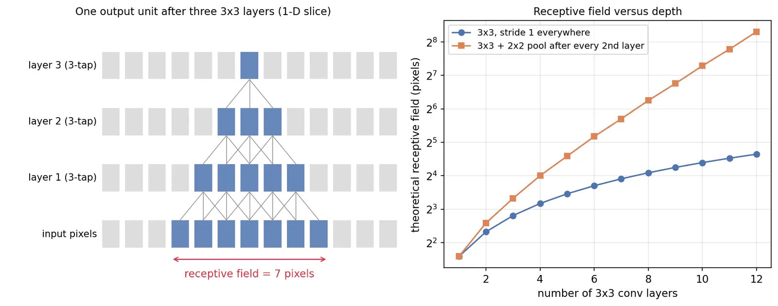

Two refinements matter in practice. First, the formula gives the theoretical receptive field. Luo et al. [12] showed that the effective receptive field, measured by how much each input pixel actually affects the output gradient, is roughly Gaussian and occupies only a fraction of the theoretical one. Pixels near the center dominate. Second, the receptive field decides what a network can use: a denoiser whose receptive field is smaller than the noise correlation length cannot remove that noise, and a classifier whose last layer sees only part of an object cannot recognize it from context.

Feature hierarchies

Because the receptive field grows with depth while resolution shrinks, a CNN builds a feature hierarchy: early layers respond to edges and color blobs (Figure 4), middle layers to textures and parts, late layers to object-level patterns over large regions. A typical backbone is organized in stages, each ending with a 2× downsampling and doubling the channel count, so features go from “high-resolution, few channels, local” to “low-resolution, many channels, semantic”. High-level tasks read the late stages. Dense prediction and low-level tasks need the early, high-resolution stages too, which is why encoder–decoders exist (below).

Landmark CNN architectures

Plain version. Between 2012 and 2016 a series of networks, each deeper than the last, won the ImageNet Large Scale Visual Recognition Challenge (ILSVRC) [6]. Each one introduced a design idea that is still in use.

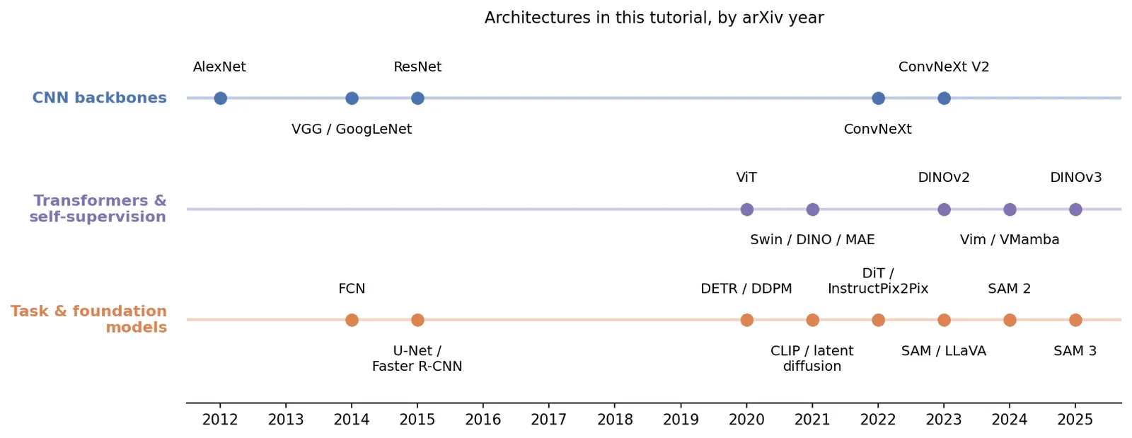
LeNet-5 and where CNNs really began

The post’s original heading said “CNN (1998~)”. That year is when LeCun, Bottou, Bengio and Haffner published LeNet-5 [5], not when CNNs started: convolutional networks trained by backpropagation were already reading handwritten ZIP-code digits in 1989 [4].

LeNet-5 is a textbook pattern-recognition system in network form [1]. Layers C1 to C5 are the feature extractor: convolutions (C1, C3, C5) alternating with subsampling layers (S2, S4) that turn a 32×32 digit image into a 120-dimensional feature vector. F6 and the output layer are the classifier. Everything, features included, is trained by gradient descent on the classification loss. This was the end-to-end idea, already in place, but it needed 15 more years of data and compute to dominate.

AlexNet (2012)

AlexNet [7] has five convolutional layers and three fully connected layers (eight learned layers, about 60 million parameters). Its ingredients were not individually new, but the combination was: ReLU activations, which train much faster than saturating sigmoids; an efficient GPU implementation; heavy data augmentation; and dropout in the fully connected layers. It won ILSVRC 2012 by a wide margin, which is why 2012 is usually given as the start of the deep-learning era in vision.

VGG (2014)

Simonyan and Zisserman [8] asked a single question: what happens if you use only $3 \times 3$ convolutions and make the network deeper? Their best configurations had 16 and 19 weight layers. The reason $3 \times 3$ is enough is the receptive-field formula above: two stacked $3 \times 3$ layers see $5 \times 5$, three see $7 \times 7$. For $C$ channels in and out, three $3 \times 3$ layers cost $3 \cdot 9 C^2 = 27C^2$ weights versus $49C^2$ for one $7 \times 7$ layer, and they insert two extra nonlinearities. VGG’s uniform design made it the default pretrained feature extractor for years.

GoogLeNet / Inception (2014)

GoogLeNet [9], 22 layers deep, won ILSVRC 2014. Its Inception module runs $1 \times 1$, $3 \times 3$ and $5 \times 5$ convolutions and a pooling branch in parallel and concatenates their outputs, so each block sees several scales at once. To keep this affordable, cheap $1 \times 1$ convolutions first reduce the number of channels. A $1 \times 1$ convolution mixes channels at each pixel without looking at neighbors; it is a per-pixel fully connected layer, and it remains a basic building block everywhere.

ResNet (2015) and why residual connections work

Deeper should be better, but in practice it was not: He et al. [10] observed that a plain 56-layer network had higher training error than a 20-layer one. That is not overfitting. It is an optimization failure: the deeper net could in principle copy the shallow one and set the extra layers to the identity, but gradient descent does not find that solution.

The fix is the residual block (Figure 7). Instead of asking a stack of layers to learn a mapping $H(\mathbf{x})$ directly, let it learn the residual $F(\mathbf{x}) = H(\mathbf{x}) - \mathbf{x}$ and add the input back:

$$\mathbf{y} = \sigma\big(\mathbf{x} + F(\mathbf{x}; W)\big),$$

where $\mathbf{x}$ is the block input, $F$ is typically conv–BN–ReLU–conv–BN with weights $W$ (BN is batch normalization), and $\sigma$ is ReLU. When channel counts or resolution change, the shortcut uses a $1 \times 1$ convolution instead of the identity.

Why it works:

• Identity is easy. If extra depth is not useful, the block only has to drive $F$ toward zero, which is far easier than making a stack of nonlinear layers imitate the identity. Initializing the last BN scale of $F$ at zero makes each block start as the identity.
• Gradients have a highway. Ignoring the final nonlinearity, $\partial \mathbf{y}/\partial \mathbf{x} = I + \partial F/\partial \mathbf{x}$. The identity term carries the gradient from the loss to early layers without passing through every weight matrix, so it does not vanish with depth.
• An ensemble view. Unrolling $L$ blocks gives a sum over many paths of different lengths, so a deep ResNet behaves partly like a collection of shallower networks.

class ResidualBlock(nn.Module):
    """Basic block: y = ReLU(x + F(x)), with F = conv-BN-ReLU-conv-BN."""
    def __init__(self, c):
        super().__init__()
        self.f = nn.Sequential(
            nn.Conv2d(c, c, 3, padding=1, bias=False), nn.BatchNorm2d(c), nn.ReLU(),
            nn.Conv2d(c, c, 3, padding=1, bias=False), nn.BatchNorm2d(c),
        )
    def forward(self, x):
        return torch.relu(x + self.f(x))

blk = ResidualBlock(16)
nn.init.zeros_(blk.f[4].weight)                  # zero the last BN scale, so F(x) = 0
x = torch.randn(2, 16, 32, 32)
print(torch.allclose(blk(x), torch.relu(x)))     # True: the block starts as the identity (then ReLU)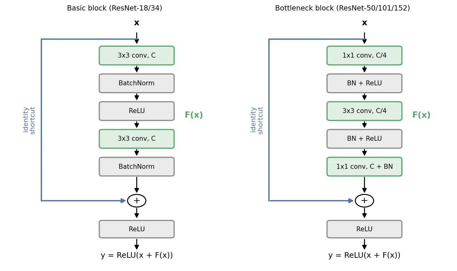

On ImageNet the paper trained ResNets with 18, 34, 50, 101 and 152 layers; the deeper three use the bottleneck block. The famous 1202-layer network appears only in the paper’s CIFAR-10 experiments [10], [11] (32×32 images), where it trained fine but overfit and tested worse than the 110-layer version. The ResNet family won ILSVRC 2015, and the residual connection is now in almost every deep network, Transformers included.

Encoder–decoders for dense prediction

Plain version. A classification backbone throws away resolution to gain meaning. For segmentation or restoration we need an answer at every pixel, so we add a second half that brings the resolution back.

Precise version. Long et al.’s fully convolutional network (FCN) [13] replaced the fully connected layers of a classifier with convolutions, so the network outputs a coarse class-score map for an input of any size, then upsampled it with learned transposed convolutions and fused it with scores from earlier, finer layers. U-Net [14] made this symmetric: a contracting encoder (conv blocks and downsampling) and an expanding decoder (upsampling and conv blocks), with skip connections that concatenate each encoder stage’s feature map to the decoder stage of the same resolution. The encoder supplies what; the skips supply where. U-Net was designed for biomedical images with few labels and strong augmentation, and the same shape now underlies medical segmentation, almost every restoration network covered in DL 04, and the denoiser inside many diffusion models.

The Vision Transformer

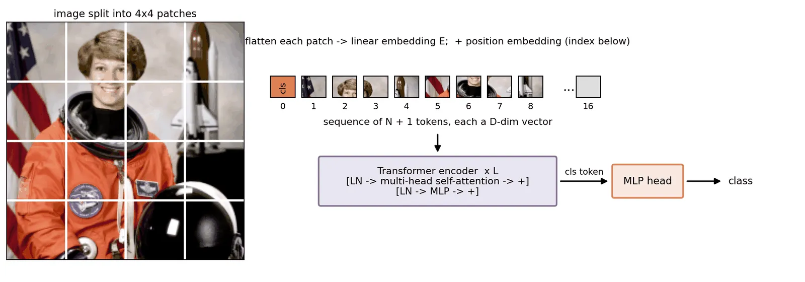
Plain version. The Transformer [15] was built for sentences: it treats the input as a sequence of tokens and lets every token look at every other token. The Vision Transformer (ViT) [16] cuts an image into small square patches, treats each patch as a “word”, and feeds the sequence to an unmodified Transformer encoder.

Patchify, embed, attend

Precise version. For an image $I \in \mathbb{R}^{C \times H \times W}$ and patch size $P$:

1. Patchify. Split $I$ into $N = HW/P^2$ non-overlapping patches and flatten each into a vector $\mathbf{p}_i \in \mathbb{R}^{CP^2}$. For a $224 \times 224$ RGB image and $P = 16$, $N = 196$ and each vector has $768$ entries.
2. Embed. Map each patch linearly to a $D$-dimensional token, $\mathbf{z}_i = E\,\mathbf{p}_i$ with $E \in \mathbb{R}^{D \times CP^2}$. Prepend a learnable class token $\mathbf{z}_{\text{cls}}$ and add learnable position embeddings $\mathbf{e}_i$, because attention by itself has no notion of where a token came from: $Z^{(0)} = [\mathbf{z}_{\text{cls}}; \mathbf{z}_1; \dots; \mathbf{z}_N] + [\mathbf{e}_0; \dots; \mathbf{e}_N]$.
3. Encode. Apply $L$ Transformer encoder blocks, each a multi-head self-attention (MSA) sublayer and an MLP sublayer, both with layer normalization (LN) and residual connections:

$$\begin{aligned} Z' &= Z^{(\ell-1)} + \mathrm{MSA}\big(\mathrm{LN}(Z^{(\ell-1)})\big),\\ Z^{(\ell)} &= Z' + \mathrm{MLP}\big(\mathrm{LN}(Z')\big). \end{aligned}$$

4. Head. Feed the final class token (or the average of all tokens) to an MLP head, which plays the role of the pattern-recognition classifier [1].

A single attention head computes, for token matrix $Z \in \mathbb{R}^{(N+1) \times D}$,

$$\mathrm{Attn}(Z) = \mathrm{softmax}\!\left(\frac{QK^\top}{\sqrt{d}}\right) V, \qquad Q = ZW_Q,\; K = ZW_K,\; V = ZW_V,$$

where $W_Q, W_K, W_V \in \mathbb{R}^{D \times d}$ are learned projections and $d$ is the head dimension. Row $i$ of the softmax matrix says how much token $i$ draws from every other token. Compared with a convolution, the “filter” is computed from the content and covers the whole image from the first layer on. The cost is quadratic in the number of tokens, $O(N^2 d)$, which is why patches rather than pixels are used.

img = torch.randn(1, 3, 224, 224)
P, D = 16, 768
patches = img.unfold(2, P, P).unfold(3, P, P)                    # (1, 3, 14, 14, 16, 16)
patches = patches.permute(0, 2, 3, 1, 4, 5).reshape(1, -1, 3 * P * P)
print(patches.shape)                                              # (1, 196, 768)
embed = nn.Conv2d(3, D, kernel_size=P, stride=P)                  # patchify + linear embed in one op
tokens = embed(img).flatten(2).transpose(1, 2)                    # (1, 196, 768)

The last two lines show a useful identity: patch embedding is a convolution with kernel size and stride both equal to $P$.

Inductive bias and the need for scale

The original post said that ViT is “harder to converge”. The more precise statement [1], [16] is about inductive bias, the assumptions built into an architecture before it sees data. A CNN assumes locality and weight sharing, so it already “knows” that nearby pixels matter together and that a pattern means the same thing anywhere in the image. ViT assumes almost nothing: apart from the patch split, all spatial structure, even the 2-D layout of the position embeddings, must be learned.

That is a trade-off, not a defect. With little data, the CNN’s assumptions are a valuable head start, and ViT trained from scratch on ImageNet-1k alone underperforms comparable ResNets. With enough data, the assumptions become a limitation, and ViT pretrained on very large datasets matched or beat the best CNNs when fine-tuned [16]. The practical lesson is that ViTs are used pretrained, either on huge labeled sets or, increasingly, with self-supervision.

Backbones after ViT

Plain version. After ViT, research went three ways: make Transformers more image-friendly (Swin), show that CNNs can catch up when modernized (ConvNeXt), and pretrain without labels so that one backbone serves every task (DINO, MAE, DINOv2/v3).

Swin Transformer: locality returns

Swin [17] computes attention only inside non-overlapping local windows (for example $7 \times 7$ tokens), which makes the cost linear in image size. In alternate blocks the window grid is shifted by half a window, so information crosses window borders. Between stages, neighboring tokens are merged to halve resolution. The result is a hierarchical, multi-scale feature pyramid shaped like a CNN backbone, which is exactly what detection and segmentation heads expect. Swin put locality and hierarchy, the CNN’s inductive biases, back into a Transformer.

ConvNeXt: the CNN counterpoint

Liu et al. [18] started from a ResNet-50 and modernized it one step at a time, using the training recipe and design choices of Transformers: a “patchify” stem (a $4 \times 4$ convolution with stride 4), large $7 \times 7$ depthwise convolutions, an inverted-bottleneck MLP, fewer activation and normalization layers, and layer normalization. The resulting pure CNN, ConvNeXt, matched Swin in accuracy and scaling on classification, detection and segmentation. The lesson: much of ViT’s advantage came from training recipes and macro design, not from attention itself. ConvNeXt V2 [18] then added masked-autoencoder pretraining adapted to convolutions (the fully convolutional masked autoencoder, FCMAE) and a global response normalization layer. Today large foundation models mostly use ViT backbones, but convolutions remain common in low-level vision and on edge devices [1].

Self-supervised pretraining: DINO versus MAE

Self-supervised learning creates a training signal from the images themselves, so no labels are needed. Two recipes dominate, and they are often confused.

DINO: self-distillation [19]. A student network $g_s$ and a teacher $g_t$ with the same architecture each output a probability vector over $K$ prototype dimensions. Several random crops of an image are made: two large “global” views and several small “local” views. The teacher sees only global views, the student sees all of them, and the student is trained to match the teacher’s output:

$$\min_{\theta_s} \sum_{x \in \{x^g_1, x^g_2\}} \;\sum_{\substack{x' \in V \\ x' \neq x}} H\big(P_t(x),\, P_s(x')\big), \qquad H(a, b) = -a^\top \log b,$$

where $V$ is the set of all views, $P_t$ and $P_s$ are the softmax outputs of teacher and student, and $\theta_s$ are the student’s weights. The teacher is not trained by gradients. Its weights are an exponential moving average of the student’s, $\theta_t \leftarrow \lambda \theta_t + (1 - \lambda)\theta_s$ with $\lambda$ close to 1, and its outputs are centered and sharpened so that training does not collapse to a constant output. Matching “small crop” to “whole image” forces the network to recognize objects from parts. A remarkable emergent property is that the attention maps of a DINO ViT segment the main objects without ever seeing a mask.

MAE: masked prediction [20]. The masked autoencoder hides a large random subset of patches (75 % works best), encodes only the visible ones with a ViT, and asks a light decoder to reconstruct the missing pixels:

$$\mathcal{L}_{\text{MAE}} = \frac{1}{|\mathcal{M}|} \sum_{i \in \mathcal{M}} \big\lVert \hat{\mathbf{p}}_i - \mathbf{p}_i \big\rVert_2^2,$$

where $\mathcal{M}$ is the set of masked patch indices, $\mathbf{p}_i$ the (normalized) pixels of patch $i$ and $\hat{\mathbf{p}}_i$ the reconstruction. This “hide and predict” game is the image analogue of masked-word prediction in language models; DINO, by contrast, is a teacher–student distillation method [1]. MAE is cheap because the encoder processes only a quarter of the tokens, and it fine-tunes very well. DINO-style features are better frozen, used as-is with a linear head.

DINOv2 and DINOv3: frozen general-purpose features

DINOv2 [21] scaled DINO-style self-distillation to a 1-billion-parameter ViT trained on a large, automatically curated image collection, then distilled it into smaller models. Its frozen features work well for both image-level tasks (classification, retrieval) and pixel-level tasks (segmentation, depth estimation) with only a light head. DINOv3 [21] scaled data and model size further and introduced Gram anchoring, a regularizer that keeps dense patch features from degrading during very long training, so the same frozen backbone gives high-quality dense features.

This closes the loop with the pattern-recognition pipeline. “Feature extractor + classifier” has returned as pretrained frozen backbone + light head. The feature extractor is now learned once, at very large scale, without labels.

State-space backbones

Vision Mamba (Vim) and VMamba [22] replace attention with selective state-space models, which scan the token sequence with cost linear in its length. Images are not sequences, so these models scan the patch grid along more than one path (Vim is bidirectional; VMamba’s 2-D selective scan traverses several routes). They are attractive for high-resolution inputs but are still mostly a research direction rather than a default backbone.

High-level vision tasks

Plain version. High-level tasks differ in how where the answer must be: one label for the whole image, a box per object, or a label for every pixel.

Task	Output	Typical loss	Typical metric	Representative models
Classification	one label (or a probability vector)	cross-entropy	top-1 / top-5 accuracy	ResNet, ViT, ConvNeXt [10], [16], [18]
Object detection	a set of (box, class, score)	classification + box regression, or set matching	average precision (AP) over IoU thresholds	Faster R-CNN, DETR [23]
Semantic segmentation	a class per pixel	per-pixel cross-entropy, Dice (an overlap loss, below)	mean IoU	FCN, U-Net [13], [14]
Instance segmentation	a mask and class per object	detection + mask losses	mask AP	promptable: SAM family [24]

Classification

Assign one label to the whole image. The network is a backbone plus global pooling plus a linear layer, trained with cross-entropy $\mathcal{L} = -\log \hat p_{y}$, where $\hat p_y$ is the predicted probability of the true class $y$. Classification is also the pretraining task that produced most backbones before self-supervision. DL 02 covers it in depth.

Object detection

Find every object, its class and its location as an axis-aligned box (a region of interest, ROI, given by its corner coordinates or center, width and height) [1]. Two design lineages illustrate the field [23]. Faster R-CNN is two-stage: a region proposal network suggests candidate boxes from shared CNN features, and a second head classifies and refines each one; duplicates are removed by non-maximum suppression. DETR treats detection as set prediction: a Transformer decoder emits a fixed set of predictions, and a bipartite matching between predictions and ground-truth objects defines the loss, which removes hand-designed anchors and non-maximum suppression. Box quality is measured by intersection over union,

$$\mathrm{IoU}(A, B) = \frac{|A \cap B|}{|A \cup B|},$$

where $A$ and $B$ are the predicted and true regions. The closely related Dice coefficient $2|A \cap B| / (|A| + |B|)$ is used, in a differentiable soft form, as a segmentation loss. Average precision summarizes the precision–recall curve at one or more IoU thresholds. Details are in DL 03.

Semantic and instance segmentation

Here the region of interest is the object’s exact set of pixels, not a box [1].

• Semantic segmentation labels each pixel with a class. Two overlapping people become one “person” region.
• Instance segmentation also separates objects of the same class. The two people become “person 1” and “person 2”.

Semantic segmentation is the natural job of the encoder–decoders above [13], [14]. Instance segmentation adds a detection-like component that proposes one mask per object.

Promptable segmentation: SAM, SAM 2, SAM 3

Segmentation now has promptable foundation models [24]. SAM (Segment Anything) takes an image and a prompt (points, a box, or a rough mask) and returns a mask for the indicated object. A heavy ViT image encoder runs once per image, and a light prompt encoder and mask decoder run per prompt, so interaction is fast. It was trained on SA-1B, a dataset of more than 1 billion masks on 11 million images, built with a model-in-the-loop “data engine”. SAM 2 extends this to video with a streaming memory that carries the object from frame to frame, trained on a new video dataset (SA-V). SAM 3 adds promptable concept segmentation: given a short noun phrase such as “yellow school bus”, image exemplars, or both, it finds, segments and (in video) tracks all matching instances, rather than the one object a click points at. With SAM 3 the line between detection, instance segmentation and tracking becomes thin; tracking is covered in DL 06.

Low-level vision tasks

Plain version. Low-level tasks take an image and return an improved or transformed image of the same scene. The output is judged pixel by pixel, or by how natural it looks.

The general formulation is an inverse problem. A degraded observation $\mathbf{y}$ is modeled as

$$\mathbf{y} = \mathcal{D}(\mathbf{x}) + \mathbf{n},$$

where $\mathbf{x}$ is the clean image, $\mathcal{D}$ a degradation operator (blur, downsampling, haze, low exposure) and $\mathbf{n}$ noise, the same model as in DIP 05. A network $f_\theta$ is trained on pairs to minimize, for example, $\lVert f_\theta(\mathbf{y}) - \mathbf{x} \rVert_1$. Because real paired data is scarce, pairs are usually synthesized by applying a modeled degradation to clean images, and the gap between synthetic and real degradations is the field’s central difficulty.

• Image restoration recovers the clean image: denoising, deblurring, super-resolution (small to large), dehazing (hazy to clear), deraining. Architectures are full-resolution encoder–decoders (U-Net-like) or residual networks without downsampling, now often with window attention. See DL 04.
• Image enhancement makes content easier to see without a single “true” target: low-light enhancement (bringing out detail in dark images, roughly a smart brightening; turning night into day would be translation instead) and underwater enhancement. See DL 05.
• Image alignment (registration) estimates the geometric transform or dense flow that maps one image onto another, a prerequisite for burst fusion, HDR and medical image comparison.
• Image-to-image translation maps an image from one domain or style to another: day to night, summer to winter, sketch to photo. Face-swapping “deepfakes” are a (misused) application of the same idea. Since diffusion models, translation and editing are often done by a generative model conditioned on the input image, as discussed next.

Generation and vision–language models

Plain version. Two newer families do not fit the old map well: models that create images from text, and models that talk about images. Both rely on large-scale pretraining and on connecting images with language.

Diffusion models: from noise to image

A denoising diffusion probabilistic model (DDPM) [27] defines a forward process that gradually adds Gaussian noise to an image $\mathbf{x}_0$ over $T$ steps. In closed form,

$$\mathbf{x}_t = \sqrt{\bar\alpha_t}\, \mathbf{x}_0 + \sqrt{1 - \bar\alpha_t}\, \boldsymbol{\epsilon}, \qquad \boldsymbol{\epsilon} \sim \mathcal{N}(\mathbf{0}, I),$$

where $t \in \{1, \dots, T\}$ is the step and $\bar\alpha_t \in (0, 1)$ is a fixed schedule that decreases from nearly 1 to nearly 0. A network $\boldsymbol{\epsilon}_\theta$ is trained to predict the noise that was added,

$$\mathcal{L} = \mathbb{E}_{\mathbf{x}_0, t, \boldsymbol{\epsilon}} \big\lVert \boldsymbol{\epsilon} - \boldsymbol{\epsilon}_\theta(\mathbf{x}_t, t) \big\rVert_2^2,$$

and generation runs the process backwards, starting from pure noise and denoising step by step. In other words, a generator is a learned denoiser applied many times, which ties generation directly to the restoration problems above.

• Latent diffusion [28] runs the diffusion in the compressed latent space of a pretrained autoencoder rather than on pixels, which cuts the cost enough for high-resolution text-to-image synthesis; text conditioning enters through cross-attention. It is the basis of Stable Diffusion.
• DiT (Diffusion Transformer) [28] replaces the U-Net denoiser with a Transformer on latent patches and shows that quality improves steadily as the model’s compute grows.
• InstructPix2Pix [29] edits a given image according to a written instruction (“make it winter”), so classic image-to-image translation becomes a special case of conditional generation.

Vision–language models

Visual question answering (VQA), answering a free-form question about an image, once required a pipeline of image features, captioning and text question answering [1]. Two steps made it a single model.

CLIP [25] trains an image encoder $f$ and a text encoder $g$ on 400 million image–text pairs with a contrastive objective. In a batch of $B$ pairs, with normalized embeddings $\mathbf{u}_i = f(I_i)$ and $\mathbf{v}_j = g(T_j)$ and temperature $\tau$, the image-to-text loss is

$$\mathcal{L}_{I \to T} = -\frac{1}{B} \sum_{i=1}^{B} \log \frac{\exp(\mathbf{u}_i^\top \mathbf{v}_i / \tau)}{\sum_{j=1}^{B} \exp(\mathbf{u}_i^\top \mathbf{v}_j / \tau)},$$

and the total loss averages it with the symmetric text-to-image term. Matching pairs are pulled together and all other pairs in the batch pushed apart. Because the label space is now “any sentence”, CLIP can classify zero-shot: embed the prompts “a photo of a cat”, “a photo of a dog”, … and pick the one closest to the image.

LLaVA [26] connects a CLIP vision encoder to a large language model (LLM) through a projection layer that maps visual tokens into the LLM’s word-embedding space, then fine-tunes on instruction-following conversations about images. Most current multimodal LLMs keep this vision encoder + projector + LLM pattern, so VQA, captioning and many recognition tasks are now handled by prompting one model.

Modern view

The trend across this tutorial is a move from “one task, one model” to “one foundation model + prompt or light head”. The surveys below are a good map of how the field got there.

CNN architectures. Li et al. [30] review CNNs from their history through the convolution operation itself, classic and advanced architectures (the LeNet–ResNet line, lightweight and attention-augmented networks), 1-D, 2-D and multi-dimensional convolutions, and applications. They also cover the improvements made to each component (layer design, activation and loss functions, regularization, optimization, fast computation), run experiments to derive rules of thumb for choosing functions and hyperparameters, and close with open issues and promising directions. It is the best single place to see the CNN design space laid out component by component.

Vision Transformers. Khan et al. [31] (ACM Computing Surveys) organize Transformer work by task: the foundations (self-attention, large-scale pretraining, bidirectional encoding), then recognition (classification, detection, segmentation, action recognition), generative modeling, multimodal tasks (VQA, visual reasoning, grounding), video, low-level vision (super-resolution, enhancement, colorization) and 3-D point clouds. Their central contrast matches this tutorial’s: Transformers model long-range dependencies with minimal inductive bias, so they need large-scale pretraining or architectural priors (windows, hierarchies) to be data-efficient.

Self-supervised visual learning. Jing and Tian [32] (TPAMI) survey the pre-2020 generation of self-supervised methods, organized by pretext task (generation-based, context-based, free-semantic-label-based and cross-modal), along with the standard protocol of evaluating features by transfer to downstream tasks. Balestriero et al. [33] cover the modern generation in a practical “cookbook” and group methods into four families: deep metric learning (contrastive), self-distillation (the DINO family), canonical-correlation-style methods, and masked image modeling (MAE). Their emphasis on the many hidden “knobs” (augmentations, projector heads, collapse prevention) explains why reproducing self-supervised results is hard.

Foundation models for vision. Awais et al. [34] (TPAMI) categorize vision foundation models by modality pairing (vision with text, audio, depth), training objective (contrastive versus generative) and prompt type: textual, visual (points, boxes, masks, as in SAM) and heterogeneous. Their open challenges are evaluation and benchmarking, real-world understanding and contextual reasoning, bias, adversarial robustness and interpretability. Zhang et al. [35] (TPAMI) focus on vision–language models for visual recognition: architectures and pretraining objectives, transfer methods (prompt tuning, adapters) and knowledge distillation into detectors and segmenters. They argue that web-scale image–text data reduces the dependence on crowd-sourced labels and lets one model serve many tasks.

State of the art, 2024–2026. Without quoting benchmark numbers, the landscape looks like this:

• Backbones. Large ViTs pretrained with self-supervision or image–text data are the default for high-level tasks, with frozen DINOv2/DINOv3 features [21] a strong baseline for dense tasks. Modern CNNs (ConvNeXt V2 [18]) remain competitive and are preferred where latency, memory or high resolution dominate. State-space backbones [22] are an active alternative.
• Segmentation and tracking have converged on promptable models: SAM 2 for video objects and SAM 3 for open-vocabulary concepts [24].
• Generation has moved to latent diffusion with Transformer denoisers [28], and editing to instruction-conditioned diffusion [29].
• Understanding is increasingly done by multimodal LLMs in the LLaVA pattern [26].
• Low-level vision still relies heavily on task-specific encoder–decoders trained on synthetic degradations, now increasingly with generative (diffusion) priors; see DL 04 and DL 05.

Open problems. (1) Data and evaluation: benchmarks saturate and may overlap with web-scale pretraining data, so it is hard to tell generalization from memorization [34]. (2) Real-world degradations: models trained on synthetic noise or blur still fail on real camera pipelines. (3) Fidelity versus hallucination: generative priors produce sharp but sometimes invented detail, which is unacceptable in medical or forensic use. (4) Efficiency: attention is quadratic in tokens, and foundation models are hard to run on devices. (5) Dense features at scale: DINOv3’s Gram anchoring [21] exists because dense feature quality can degrade as training scales. (6) Bias, robustness and interpretability of models trained on uncurated web data [34].

Key takeaways

• Deep learning reduces the three classical levels to two: low-level (image → image, judged by fidelity) and high-level (image → semantics, judged by accuracy). Mid-level analysis goes to whichever its output resembles.
• End-to-end learning replaced hand-designed features with learned ones. The split returned at scale as pretrained backbone + light head.
• A convolutional layer is a bank of learned spatial filters with local connectivity and weight sharing. Stride, padding and pooling set the output size; the receptive field grows as $r_\ell = r_{\ell-1} + (k_\ell - 1) j_{\ell-1}$, and the effective field is smaller than the theoretical one.
• LeNet-5 (1998) was not the first CNN; backprop-trained convolutional networks date to 1989. ResNet was trained at 18/34/50/101/152 layers on ImageNet; 1202 layers appears only on CIFAR-10. Residual connections make the identity easy and give gradients a direct path.
• Encoder–decoders with skip connections (FCN, U-Net) are the standard shape for dense prediction and restoration.
• ViT has little inductive bias, so it needs large-scale pretraining. Swin added locality back; ConvNeXt showed a modernized CNN matches it.
• DINO is teacher–student self-distillation; MAE is masked prediction. DINOv2/v3 provide frozen, general-purpose features.
• Tasks increasingly converge on promptable or language-connected foundation models: SAM 1/2/3 for segmentation, latent diffusion and DiT for generation, CLIP and LLaVA for vision–language.

Exercises

1. Receptive field by hand. A network has, in order: conv $7 \times 7$ stride 2; max-pool $3 \times 3$ stride 2; then four conv $3 \times 3$ stride 1. Compute the theoretical receptive field and the jump after each layer, and check your answer with the receptive_field function.

Hint

Start with $r = 1$, $j = 1$. After the first conv: $r = 7$, $j = 2$. After pooling: $r = 7 + 2 \cdot 2 = 11$, $j = 4$. Each following $3 \times 3$ layer adds $2 \cdot 4 = 8$, so $r = 19, 27, 35, 43$ with $j = 4$.

2. Parameter budget. For $C = 256$ input and output channels, compare the weights (ignore biases) of one $5 \times 5$ convolution, two stacked $3 \times 3$ convolutions, and a bottleneck ($1 \times 1$ to 64 channels, $3 \times 3$ at 64, $1 \times 1$ back to 256). Which have the same receptive field?

Hint

$25C^2 \approx 1.64$M; $2 \cdot 9C^2 \approx 1.18$M; bottleneck $256 \cdot 64 + 9 \cdot 64^2 + 64 \cdot 256 \approx 0.07$M. The first two both see $5 \times 5$; the bottleneck sees $3 \times 3$ but is far cheaper, which is why ResNet-50 and deeper use it.

3. Why the identity is hard without a shortcut. Inside a network, a block’s input usually comes from a previous ReLU, so it is non-negative. Show that for such inputs a residual block with $F \equiv 0$ outputs exactly $\mathbf{y} = \mathbf{x}$. Then explain what a plain block (conv–BN–ReLU–conv–BN–ReLU) would have to learn to output $\mathbf{y} = \mathbf{x}$. What does this imply for very deep plain networks?

Hint

For $\mathbf{x} \ge 0$, $\mathrm{ReLU}(\mathbf{x} + 0) = \mathbf{x}$. A plain block must instead learn weights that exactly undo two convolutions and two normalizations, a precise and fragile solution that gradient descent rarely finds. The residual block only needs $F = 0$, which weight decay and zero-initialization already push it toward. Deep plain networks therefore struggle to “do nothing” in extra layers, which matches the degradation the ResNet authors observed.

4. ViT token count and cost. For a $512 \times 512$ input, compute the number of tokens for patch sizes 32, 16 and 8, and the relative cost of one global attention layer ($\propto N^2$). How does Swin’s windowed attention with $7 \times 7$ windows change the scaling?

Hint

$N = (512/P)^2$: 256, 1024, 4096 tokens; costs scale 1 : 16 : 256. Windowed attention costs $N \cdot 49$ per layer (each token attends to 49 others), so it grows linearly with $N$.

5. Learned versus hand-set filters. Modify the digit CNN so that its first layer is frozen to four hand-set kernels (two Sobels, a Laplacian and a box blur) plus four random kernels. Train only the rest. Compare test accuracy with the fully learned network and inspect what happens to the random kernels if you unfreeze them.

Hint

Set conv.weight.requires_grad_(False) after assigning the weights, and pass only the remaining parameters to the optimizer. On this easy dataset both versions reach similar accuracy; the point is that hand-set derivative filters are a reasonable first layer, and that unfrozen random kernels tend to drift toward oriented, derivative-like patterns (compare Figure 4).

6. Choose a recipe. You have 2,000 labeled microscopy images and need (a) a per-image quality label, (b) per-pixel cell masks, (c) denoised images. For each, propose a backbone, a head and a training strategy using this tutorial’s map, and say which would benefit most from a frozen self-supervised backbone.

Hint

(a) Frozen DINOv2/v3 or fine-tuned ConvNeXt + linear head. (b) U-Net, possibly with a pretrained encoder, or SAM prompted by points and then fine-tuned. (c) A full-resolution restoration network trained on synthetic noisy/clean pairs that match the microscope’s noise. Frozen semantic features help (a) and (b) most; (c) depends on pixel-accurate statistics more than on semantics.

References

1. Shyandram, “深度學習的數位影像處理介紹 (An introduction to digital image processing with deep learning),” blog post, 2024; updated 2026. link
2. R. C. Gonzalez and R. E. Woods, Digital Image Processing, 4th ed., Pearson, 2018. publisher page
3. S. Theodoridis and K. Koutroumbas, Pattern Recognition, 4th ed., Academic Press, 2008. publisher page
4. Y. LeCun, B. Boser, J. S. Denker, D. Henderson, R. E. Howard, W. Hubbard, and L. D. Jackel, “Backpropagation applied to handwritten zip code recognition,” Neural Computation, vol. 1, no. 4, pp. 541–551, 1989. doi:10.1162/neco.1989.1.4.541
5. Y. LeCun, L. Bottou, Y. Bengio, and P. Haffner, “Gradient-based learning applied to document recognition,” Proceedings of the IEEE, vol. 86, no. 11, pp. 2278–2324, 1998. doi:10.1109/5.726791
6. O. Russakovsky, J. Deng, H. Su, et al., “ImageNet large scale visual recognition challenge,” International Journal of Computer Vision, vol. 115, no. 3, pp. 211–252, 2015. doi:10.1007/s11263-015-0816-y · arXiv:1409.0575
7. A. Krizhevsky, I. Sutskever, and G. E. Hinton, “ImageNet classification with deep convolutional neural networks,” NeurIPS, 2012. proceedings
8. K. Simonyan and A. Zisserman, “Very deep convolutional networks for large-scale image recognition,” ICLR, 2015. arXiv:1409.1556
9. C. Szegedy, W. Liu, Y. Jia, P. Sermanet, S. Reed, D. Anguelov, D. Erhan, V. Vanhoucke, and A. Rabinovich, “Going deeper with convolutions,” CVPR, 2015. doi:10.1109/CVPR.2015.7298594 · arXiv:1409.4842
10. K. He, X. Zhang, S. Ren, and J. Sun, “Deep residual learning for image recognition,” CVPR, 2016. doi:10.1109/CVPR.2016.90 · arXiv:1512.03385
11. A. Krizhevsky, “Learning multiple layers of features from tiny images,” technical report, University of Toronto, 2009 (the CIFAR-10/100 datasets). dataset page
12. W. Luo, Y. Li, R. Urtasun, and R. Zemel, “Understanding the effective receptive field in deep convolutional neural networks,” NeurIPS, 2016. arXiv:1701.04128
13. J. Long, E. Shelhamer, and T. Darrell, “Fully convolutional networks for semantic segmentation,” CVPR, 2015. arXiv:1411.4038
14. O. Ronneberger, P. Fischer, and T. Brox, “U-Net: Convolutional networks for biomedical image segmentation,” MICCAI, 2015. arXiv:1505.04597
15. A. Vaswani, N. Shazeer, N. Parmar, J. Uszkoreit, L. Jones, A. N. Gomez, Ł. Kaiser, and I. Polosukhin, “Attention is all you need,” NeurIPS, 2017. ML anthology
16. A. Dosovitskiy, L. Beyer, A. Kolesnikov, D. Weissenborn, X. Zhai, T. Unterthiner, M. Dehghani, M. Minderer, G. Heigold, S. Gelly, J. Uszkoreit, and N. Houlsby, “An image is worth 16x16 words: Transformers for image recognition at scale,” ICLR, 2021. arXiv:2010.11929
17. Z. Liu, Y. Lin, Y. Cao, H. Hu, Y. Wei, Z. Zhang, S. Lin, and B. Guo, “Swin Transformer: Hierarchical vision Transformer using shifted windows,” ICCV, 2021. doi:10.1109/ICCV48922.2021.00986 · arXiv:2103.14030
18. Z. Liu, H. Mao, C.-Y. Wu, C. Feichtenhofer, T. Darrell, and S. Xie, “A ConvNet for the 2020s,” CVPR, 2022, arXiv:2201.03545; and S. Woo, S. Debnath, R. Hu, X. Chen, Z. Liu, I. S. Kweon, and S. Xie, “ConvNeXt V2: Co-designing and scaling ConvNets with masked autoencoders,” CVPR, 2023, arXiv:2301.00808.
19. M. Caron, H. Touvron, I. Misra, H. Jégou, J. Mairal, P. Bojanowski, and A. Joulin, “Emerging properties in self-supervised vision Transformers,” ICCV, 2021. doi:10.1109/ICCV48922.2021.00951 · arXiv:2104.14294
20. K. He, X. Chen, S. Xie, Y. Li, P. Dollár, and R. Girshick, “Masked autoencoders are scalable vision learners,” CVPR, 2022. doi:10.1109/CVPR52688.2022.01553 · arXiv:2111.06377
21. M. Oquab, T. Darcet, T. Moutakanni, et al., “DINOv2: Learning robust visual features without supervision,” Transactions on Machine Learning Research, 2024, arXiv:2304.07193; and O. Siméoni, H. V. Vo, M. Seitzer, F. Baldassarre, M. Oquab, et al., “DINOv3,” arXiv preprint, 2025, arXiv:2508.10104.
22. L. Zhu, B. Liao, Q. Zhang, X. Wang, W. Liu, and X. Wang, “Vision Mamba: Efficient visual representation learning with bidirectional state space model,” ICML, 2024, arXiv:2401.09417; and Y. Liu, Y. Tian, Y. Zhao, H. Yu, L. Xie, Y. Wang, Q. Ye, J. Jiao, and Y. Liu, “VMamba: Visual state space model,” NeurIPS, 2024, arXiv:2401.10166.
23. S. Ren, K. He, R. Girshick, and J. Sun, “Faster R-CNN: Towards real-time object detection with region proposal networks,” NeurIPS, 2015, arXiv:1506.01497; and N. Carion, F. Massa, G. Synnaeve, N. Usunier, A. Kirillov, and S. Zagoruyko, “End-to-end object detection with Transformers,” ECCV, 2020, arXiv:2005.12872.
24. A. Kirillov, E. Mintun, N. Ravi, et al., “Segment anything,” ICCV, 2023, arXiv:2304.02643; N. Ravi, V. Gabeur, Y.-T. Hu, R. Hu, et al., “SAM 2: Segment anything in images and videos,” ICLR, 2025, arXiv:2408.00714; and N. Carion, L. Gustafson, Y.-T. Hu, S. Debnath, et al., “SAM 3: Segment anything with concepts,” ICLR, 2026, arXiv:2511.16719.
25. A. Radford, J. W. Kim, C. Hallacy, A. Ramesh, G. Goh, et al., “Learning transferable visual models from natural language supervision,” ICML, 2021. arXiv:2103.00020
26. H. Liu, C. Li, Q. Wu, and Y. J. Lee, “Visual instruction tuning,” NeurIPS, 2023. arXiv:2304.08485
27. J. Ho, A. Jain, and P. Abbeel, “Denoising diffusion probabilistic models,” NeurIPS, 2020. arXiv:2006.11239
28. R. Rombach, A. Blattmann, D. Lorenz, P. Esser, and B. Ommer, “High-resolution image synthesis with latent diffusion models,” CVPR, 2022, arXiv:2112.10752; and W. Peebles and S. Xie, “Scalable diffusion models with Transformers,” ICCV, 2023, arXiv:2212.09748.
29. T. Brooks, A. Holynski, and A. A. Efros, “InstructPix2Pix: Learning to follow image editing instructions,” CVPR, 2023. arXiv:2211.09800
30. Z. Li, F. Liu, W. Yang, S. Peng, and J. Zhou, “A survey of convolutional neural networks: Analysis, applications, and prospects,” IEEE Transactions on Neural Networks and Learning Systems, vol. 33, 2022. doi:10.1109/TNNLS.2021.3084827 · arXiv:2004.02806
31. S. Khan, M. Naseer, M. Hayat, S. W. Zamir, F. S. Khan, and M. Shah, “Transformers in vision: A survey,” ACM Computing Surveys, vol. 54, no. 10s, 2022. doi:10.1145/3505244 · arXiv:2101.01169
32. L. Jing and Y. Tian, “Self-supervised visual feature learning with deep neural networks: A survey,” IEEE Transactions on Pattern Analysis and Machine Intelligence, vol. 43, 2021. doi:10.1109/TPAMI.2020.2992393 · arXiv:1902.06162
33. R. Balestriero, M. Ibrahim, V. Sobal, et al., “A cookbook of self-supervised learning,” arXiv preprint, 2023. arXiv:2304.12210
34. M. Awais, M. Naseer, S. Khan, R. M. Anwer, H. Cholakkal, M. Shah, M.-H. Yang, and F. S. Khan, “Foundation models defining a new era in vision: A survey and outlook,” IEEE Transactions on Pattern Analysis and Machine Intelligence, vol. 47, 2025. doi:10.1109/TPAMI.2024.3506283 · arXiv:2307.13721
35. J. Zhang, J. Huang, S. Jin, and S. Lu, “Vision-language models for vision tasks: A survey,” IEEE Transactions on Pattern Analysis and Machine Intelligence, vol. 46, 2024. doi:10.1109/TPAMI.2024.3369699 · arXiv:2304.00685
36. scikit-learn developers, “sklearn.datasets.load_digits” (a copy of the test set of the UCI optical recognition of handwritten digits dataset). docs