Chapter 4 · Filtering in the Frequency Domain

What you’ll learn

• What the Fourier transform says about a signal, and why “frequency” is a useful way to describe an image
• How sampling works, what the Nyquist rate is, and why too few samples cause aliasing and moiré
• The discrete Fourier transform (DFT) in one and two dimensions, and the properties you use every day: centering, symmetry, spectrum and phase, and the convolution theorem
• The step-by-step recipe for filtering in the frequency domain, including the padding that prevents wraparound error
• Lowpass, highpass, homomorphic, bandreject and notch filters, and why the “ideal” filter rings
• How the fast Fourier transform (FFT) makes all of this cheap, and where Fourier ideas show up in modern deep learning

The big picture

In Chapter 3 we filtered images by sliding a small kernel over the pixels. This chapter looks at the same image from a completely different angle. Instead of asking “what is the brightness at this pixel?”, we ask “how much of each kind of wave does this image contain?” That second description is called the image’s spectrum, and the tool that produces it is the Fourier transform.

Why bother? Three reasons. First, some operations are much easier to describe as “keep these frequencies, remove those” than as a kernel. Second, by the convolution theorem, a large convolution becomes a simple multiplication, which the FFT makes fast. Third, the frequency view explains things that are mysterious in the pixel view: why shrinking an image creates strange patterns, why a sharp cutoff filter produces ripples, and why a repeating stripe of noise can be removed almost perfectly. The chapter follows the arrangement of Gonzalez and Woods [1].

Background

Plain version. Any reasonable signal can be built by adding up sine and cosine waves of different frequencies, each with its own strength and starting point. The Fourier transform finds those strengths and starting points.

In the early 1800s Joseph Fourier claimed that a periodic function can be written as a weighted sum of sines and cosines, and that even non-periodic functions with finite area under the curve can be written as an integral of sines and cosines. The striking part is that nothing is lost: you can go forward to the frequency description and back again exactly.

For images this matters in two ways. A low frequency is a wave that changes slowly across the image: it carries overall brightness and large smooth regions. A high frequency changes quickly: it carries edges, fine texture and noise. Smoothing an image means weakening the high frequencies. Sharpening means strengthening them. This chapter makes that statement precise.

Fourier analysis only became a practical image-processing tool after the fast Fourier transform appeared in 1965 [4]. Before that, computing a transform of an image was far too slow. Heideman, Johnson and Burrus later showed that Gauss had used the same idea around 1805, long before computers [5].

Preliminary concepts

Plain version. Before we can transform images, we need five tools: complex numbers (to store a wave’s strength and starting point together), Fourier series (sums of waves), impulses (perfect “spikes”), the Fourier transform itself, and convolution.

Complex numbers

A complex number is $C = R + jI$, where $R$ is the real part, $I$ is the imaginary part, and $j = \sqrt{-1}$. It can also be written in polar form

$$C = |C|\, e^{j\theta}, \qquad |C| = \sqrt{R^2 + I^2}, \qquad \theta = \arctan(I / R)$$

where $|C|$ is the magnitude (length) and $\theta$ is the angle. Euler’s formula $e^{j\theta} = \cos\theta + j\sin\theta$ links the two forms. This is why the Fourier transform uses complex exponentials: one complex number holds both the amplitude of a wave and its phase (where it starts). The complex conjugate is $C^* = R - jI$.

Fourier series

A function $f(t)$ that repeats with period $T$ can be written as

$$f(t) = \sum_{n=-\infty}^{\infty} c_n\, e^{j \frac{2\pi n}{T} t}, \qquad c_n = \frac{1}{T} \int_{-T/2}^{T/2} f(t)\, e^{-j \frac{2\pi n}{T} t}\, dt$$

where $n$ is an integer, $c_n$ is the (complex) coefficient of the wave that completes $n$ cycles per period, and $t$ is the continuous variable (time or position).

Impulses and the sifting property

A continuous unit impulse $\delta(t)$ is an idealized spike: zero everywhere except at $t = 0$, with total area 1, so $\int_{-\infty}^{\infty} \delta(t)\, dt = 1$. Its most useful property is sifting:

$$\int_{-\infty}^{\infty} f(t)\, \delta(t - t_0)\, dt = f(t_0)$$

where $t_0$ is any location. Multiplying by a shifted impulse and integrating “picks out” the value of $f$ at $t_0$. The discrete impulse $\delta(x)$ is 1 at $x = 0$ and 0 elsewhere, and sifting becomes $\sum_x f(x)\,\delta(x - x_0) = f(x_0)$.

An impulse train $s_{\Delta T}(t) = \sum_{n=-\infty}^{\infty} \delta(t - n\Delta T)$ is a row of impulses spaced $\Delta T$ apart. It is the mathematical model of sampling.

The Fourier transform of a continuous function

The Fourier transform of $f(t)$ and its inverse are

$$F(\mu) = \int_{-\infty}^{\infty} f(t)\, e^{-j 2\pi \mu t}\, dt, \qquad f(t) = \int_{-\infty}^{\infty} F(\mu)\, e^{j 2\pi \mu t}\, d\mu$$

where $\mu$ is the continuous frequency (cycles per unit of $t$) and $F(\mu)$ is complex in general. Together the two equations are called a Fourier transform pair, written $f(t) \Leftrightarrow F(\mu)$.

A worked example builds intuition. Take a box of height $A$ that is nonzero for $|t| \le W/2$. Its transform is

$$F(\mu) = A W\, \frac{\sin(\pi \mu W)}{\pi \mu W} = A W\, \operatorname{sinc}(\mu W)$$

where $\operatorname{sinc}(m) = \sin(\pi m)/(\pi m)$. Two lessons follow. A function with sharp edges has a transform that spreads out with slowly decaying ripples. And there is an inverse relationship: a wider box gives a narrower sinc. Narrow in one domain means wide in the other. We will meet both lessons again when the “ideal” filter rings.

Two more pairs are worth memorizing. The transform of an impulse is a constant: $\delta(t) \Leftrightarrow 1$. And the transform of an impulse train with spacing $\Delta T$ is another impulse train with spacing $1/\Delta T$:

$$s_{\Delta T}(t) \Leftrightarrow S(\mu) = \frac{1}{\Delta T} \sum_{n=-\infty}^{\infty} \delta\!\left(\mu - \frac{n}{\Delta T}\right)$$

Convolution

The convolution of two continuous functions is

$$(f \star h)(t) = \int_{-\infty}^{\infty} f(\tau)\, h(t - \tau)\, d\tau$$

where $\tau$ is a dummy integration variable. The convolution theorem says

$$(f \star h)(t) \Leftrightarrow H(\mu) F(\mu), \qquad f(t)\, h(t) \Leftrightarrow (H \star F)(\mu)$$

Convolution in one domain is multiplication in the other. This single fact is the reason frequency-domain filtering exists.

Sampling and the Fourier transform of sampled functions

Plain version. A camera does not record a continuous scene; it measures it at a grid of points. If the points are too far apart, fast details get confused with slow ones and you see patterns that are not really there. Sample at more than twice the fastest frequency and you can, in principle, rebuild the original exactly.

Sampling as multiplication

Model sampling as multiplying $f(t)$ by an impulse train:

$$\tilde f(t) = f(t)\, s_{\Delta T}(t) = \sum_{n=-\infty}^{\infty} f(n\Delta T)\, \delta(t - n\Delta T)$$

where $\Delta T$ is the sampling interval and $f(n\Delta T)$ are the samples. By the convolution theorem, multiplication becomes convolution with $S(\mu)$, and convolving with a train of impulses just copies the spectrum:

$$\tilde F(\mu) = \frac{1}{\Delta T} \sum_{n=-\infty}^{\infty} F\!\left(\mu - \frac{n}{\Delta T}\right)$$

So the spectrum of a sampled function is an infinite, periodic sequence of copies of the original spectrum, spaced $1/\Delta T$ apart.

The sampling theorem and the Nyquist rate

Suppose $f$ is band-limited: $F(\mu) = 0$ for $|\mu| > \mu_{\max}$. The copies do not overlap as long as their spacing exceeds the width of one copy:

$$\frac{1}{\Delta T} > 2\mu_{\max}$$

This is the sampling theorem, made famous in engineering by Shannon [2]. The quantity $2\mu_{\max}$ is the Nyquist rate. Sampling faster than it means the samples contain all the information in $f$.

Reconstruction

If the copies do not overlap, multiplying $\tilde F(\mu)$ by a box $H(\mu)$ of height $\Delta T$ that covers $[-\mu_{\max}, \mu_{\max}]$ isolates the original spectrum. In the time domain this is convolution with a sinc, giving the interpolation formula

$$f(t) = \sum_{n=-\infty}^{\infty} f(n\Delta T)\, \operatorname{sinc}\!\left[\frac{t - n\Delta T}{\Delta T}\right]$$

Every sample contributes a sinc centered on itself, and the sum passes through all samples exactly. Unser’s review [3] explains how modern practice replaces the impractical infinite sinc with splines and other compact kernels that approximate it well.

Aliasing

If $1/\Delta T \le 2\mu_{\max}$, neighboring copies overlap and their tails add together. No filter can separate them afterwards: high frequencies now masquerade as low ones. This is aliasing. The only cure is prevention: remove the high frequencies with a lowpass (anti-aliasing) filter before sampling.

A one-line experiment shows the disguise. Sample a 9 Hz cosine at 10 samples per second, where the Nyquist limit is 5 Hz:

import numpy as np

fs = 10.0                      # samples per second
t = np.arange(0, 2, 1 / fs)    # 2 seconds of samples
x = np.cos(2 * np.pi * 9 * t)  # a 9 Hz tone: above fs/2 = 5 Hz
X = np.abs(np.fft.rfft(x))
freqs = np.fft.rfftfreq(len(x), d=1 / fs)
print("peak at", freqs[X.argmax()], "Hz")   # -> 1.0 Hz, not 9 Hz

The 9 Hz tone is indistinguishable from a 1 Hz tone at these sample times. This is the same effect that makes wagon wheels appear to spin backwards in films.

The discrete Fourier transform of one variable

Plain version. A computer only has a finite list of samples, so it uses a finite version of the Fourier transform. The DFT takes $M$ numbers and returns $M$ numbers, each saying how much of one particular wave is present.

Definition

For samples $f(0), f(1), \dots, f(M-1)$:

$$F(u) = \sum_{x=0}^{M-1} f(x)\, e^{-j 2\pi u x / M}, \qquad f(x) = \frac{1}{M} \sum_{u=0}^{M-1} F(u)\, e^{j 2\pi u x / M}$$

where $x = 0, \dots, M-1$ indexes samples, $u = 0, \dots, M-1$ indexes discrete frequencies (frequency $u$ completes $u$ cycles over the $M$ samples), and the factor $1/M$ sits on the inverse (other conventions split it as $1/\sqrt{M}$ on each side).

Relation to sampling

Where does this come from? Take the transform of the sampled function $\tilde F(\mu)$, which is continuous and periodic with period $1/\Delta T$. Sample one period of it at $M$ equally spaced points, $\mu = m / (M\Delta T)$ for $m = 0, \dots, M-1$. The result is exactly the DFT above. So the DFT is samples of one period of the transform of the sampled data. The spacing between DFT frequencies is

$$\Delta u = \frac{1}{M \Delta T}$$

where $M\Delta T$ is the total duration covered by the samples. Longer recordings give finer frequency resolution.

Two consequences matter in practice. Because we sampled in frequency as well, the DFT treats the data as if it repeats with period $M$. And both $F(u)$ and $f(x)$ are periodic: $F(u) = F(u + M)$ and $f(x) = f(x + M)$.

The definition is just a matrix-vector product, which is easy to check:

import numpy as np

def dft(f):
    M = len(f)
    x = np.arange(M)
    u = x.reshape(-1, 1)
    W = np.exp(-2j * np.pi * u * x / M)   # M x M matrix of complex exponentials
    return W @ f

f = np.random.default_rng(0).standard_normal(64)
print(np.allclose(dft(f), np.fft.fft(f)))  # True

Extension to functions of two variables

Plain version. Images have two directions, so the waves have two frequencies: one across and one down. A 2-D wave looks like a set of parallel stripes; its two frequencies set how close the stripes are and which way they point.

The 2-D impulse and continuous transform

The 2-D impulse $\delta(t, z)$ has unit volume and sifts like its 1-D cousin: $\iint f(t, z)\, \delta(t - t_0, z - z_0)\, dt\, dz = f(t_0, z_0)$. The 2-D continuous transform is

$$F(\mu, \nu) = \int_{-\infty}^{\infty}\!\int_{-\infty}^{\infty} f(t, z)\, e^{-j 2\pi(\mu t + \nu z)}\, dt\, dz$$

where $t, z$ are the spatial coordinates and $\mu, \nu$ are the corresponding frequencies.

2-D sampling and aliasing

Sampling on a grid with spacings $\Delta T$ and $\Delta Z$ replicates the spectrum on a 2-D lattice. A band-limited image (zero outside $|\mu| \le \mu_{\max}$, $|\nu| \le \nu_{\max}$) is recoverable when

$$\frac{1}{\Delta T} > 2\mu_{\max}, \qquad \frac{1}{\Delta Z} > 2\nu_{\max}$$

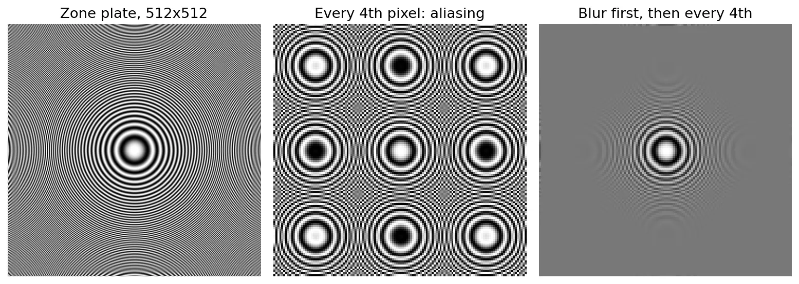
Images break this rule constantly. Real scenes contain sharp edges, which are not band-limited at all, so every digital image has some aliasing. It becomes visible when you downsample (shrink) an image by dropping pixels. Figure 4.1 uses a zone plate, a pattern whose frequency increases with distance from the center. Keeping every 4th pixel turns the fine outer rings into false circles that were never in the original. Blurring first removes the frequencies that cannot survive, and the false rings disappear.

Moiré patterns

A moiré pattern is aliasing you can see in everyday life: when a fine periodic texture (a shirt’s weave, a screen door, the halftone dots of a printed photo) is sampled by a sensor grid of similar spacing, the two periodicities beat against each other and produce large, slow, wavy bands. The middle panel of Figure 4.1 is a moiré pattern of exactly this kind. Cameras reduce it with an optical anti-aliasing filter in front of the sensor; software reduces it by blurring before resizing.

The 2-D DFT

For an $M \times N$ image $f(x, y)$:

$$F(u, v) = \sum_{x=0}^{M-1}\sum_{y=0}^{N-1} f(x, y)\, e^{-j 2\pi\left(\frac{ux}{M} + \frac{vy}{N}\right)}, \qquad f(x, y) = \frac{1}{MN} \sum_{u=0}^{M-1}\sum_{v=0}^{N-1} F(u, v)\, e^{j 2\pi\left(\frac{ux}{M} + \frac{vy}{N}\right)}$$

where $x, y$ are pixel coordinates (rows, columns), $u, v$ are discrete frequency indices, and $F(u, v)$ is an $M \times N$ array of complex numbers. Every pixel of $F$ describes one 2-D wave covering the whole image.

Properties of the 2-D DFT

Plain version. The spectrum behaves in predictable ways. Moving an object does not change the spectrum’s magnitude. Rotating the object rotates the spectrum. The center of the (shifted) spectrum holds the average brightness. And the most surprising fact: most of what we recognize in a picture is stored in the phase, not the magnitude.

Spatial and frequency intervals

If the image was sampled with spacings $\Delta T$ and $\Delta Z$, the frequency spacings of the DFT are

$$\Delta u = \frac{1}{M \Delta T}, \qquad \Delta v = \frac{1}{N \Delta Z}$$

A larger field of view gives finer frequency resolution; finer pixels extend the highest frequency the DFT can represent.

Translation and rotation

Shifting the image multiplies the transform by a linear phase, and vice versa:

$$f(x - x_0, y - y_0) \Leftrightarrow F(u, v)\, e^{-j 2\pi\left(\frac{u x_0}{M} + \frac{v y_0}{N}\right)}$$

where $(x_0, y_0)$ is the shift. Because $|e^{-j\cdot}| = 1$, the magnitude $|F|$ is unchanged by translation; only the phase changes. With polar coordinates $x = r\cos\theta$, $y = r\sin\theta$ and $u = \omega\cos\varphi$, $v = \omega\sin\varphi$, rotating $f$ by $\theta_0$ rotates $F$ by the same angle: $f(r, \theta + \theta_0) \Leftrightarrow F(\omega, \varphi + \theta_0)$.

Periodicity and centering

The DFT and its inverse are periodic in both directions: $F(u, v) = F(u + k_1 M, v + k_2 N)$ for any integers $k_1, k_2$. A raw DFT array therefore has its zero frequency in the top-left corner, with four quarter-periods meeting at the center. For viewing and for designing filters it is much easier to move zero frequency to the center. Using the translation property with $x_0 = M/2$, $y_0 = N/2$:

$$f(x, y)\,(-1)^{x + y} \Leftrightarrow F(u - M/2,\; v - N/2)$$

which holds for even $M$ and $N$. In NumPy, np.fft.fftshift does the same reordering after the transform.

Symmetry

For a real image, the transform is conjugate symmetric: $F(-u, -v) = F^*(u, v)$. Its magnitude is therefore even, $|F(-u, -v)| = |F(u, v)|$, and its phase is odd. Every spike in a spectrum comes with a mirror twin through the center. You will use this when designing notch filters.

Fourier spectrum and phase angle

Write $F(u, v) = R(u, v) + jI(u, v)$. Then

$$|F(u, v)| = \sqrt{R^2 + I^2}, \qquad \phi(u, v) = \arctan\!\left[\frac{I(u, v)}{R(u, v)}\right], \qquad P(u, v) = |F(u, v)|^2$$

are the Fourier spectrum (magnitude), the phase angle and the power spectrum. The zero-frequency term is the DC component, $F(0, 0) = MN\, \bar f$, where $\bar f$ is the mean intensity. Because $F(0,0)$ is usually thousands of times larger than everything else, spectra are displayed as $\log(1 + |F|)$.

import numpy as np
from skimage import data, img_as_float

f = img_as_float(data.camera())
F = np.fft.fft2(f)
Fc = np.fft.fftshift(F)                       # move (0,0) to the centre
spectrum = np.log1p(np.abs(Fc))               # log(1+|F|) for display
phase = np.angle(Fc)

M, N = f.shape
y, x = np.mgrid[0:M, 0:N]
print(np.allclose(np.fft.fft2(f * (-1.0) ** (x + y)), Fc))  # True for even M, N
print(np.isclose(F[0, 0].real, f.sum()))                    # DC term = sum of pixels

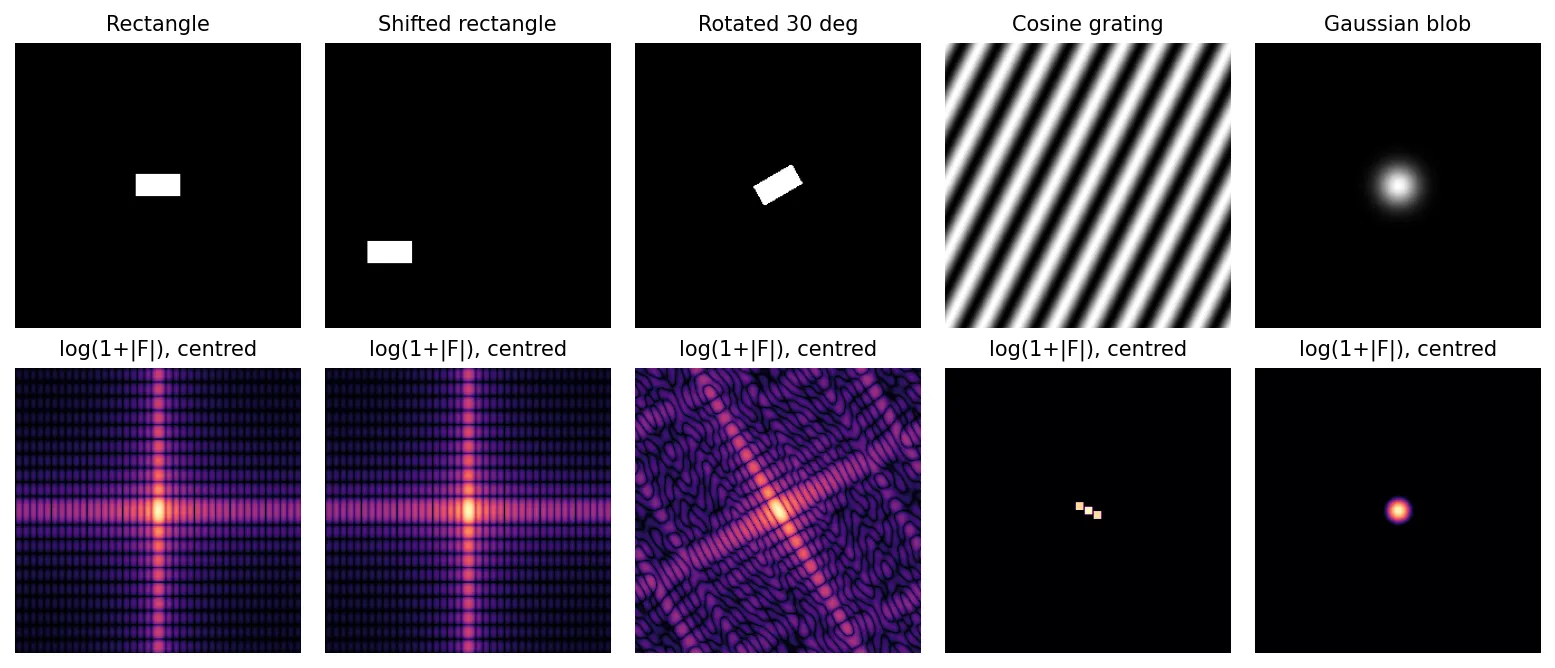
Figure 4.2 shows how simple patterns map to spectra. A rectangle gives a 2-D sinc: a bright cross whose arms are longer along the rectangle’s short side (narrow in space, wide in frequency). Shifting the rectangle leaves the spectrum identical. Rotating it rotates the spectrum. A cosine grating is a single 2-D frequency, so its spectrum is just three dots: the DC term and a symmetric pair. A Gaussian transforms into another Gaussian.

The phase-versus-magnitude experiment

Which part of the transform carries the content we recognize? Take two images, keep the magnitude of one and the phase of the other, and invert. Oppenheim and Lim made this experiment famous [7].

import numpy as np
from skimage import color, data, img_as_float

a = img_as_float(data.camera())
b = img_as_float(color.rgb2gray(data.astronaut()))
A, B = np.fft.fft2(a), np.fft.fft2(b)
mixed = np.real(np.fft.ifft2(np.abs(A) * np.exp(1j * np.angle(B))))
# 'mixed' looks like the astronaut, not the cameraman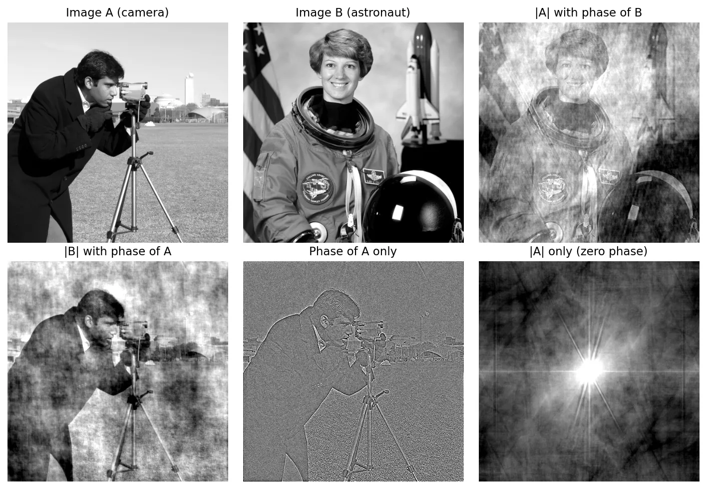

The result is unambiguous: phase carries the structure. The magnitude tells you how much energy sits at each frequency, which is roughly similar for most natural photos. The phase tells you where the waves line up, and edges are exactly the places where many waves line up. This is why the filters below are designed to leave phase untouched.

The 2-D convolution theorem

The discrete version of the convolution theorem is

$$(f \star h)(x, y) \Leftrightarrow F(u, v)\, H(u, v), \qquad (f \star h)(x, y) = \sum_{m=0}^{M-1}\sum_{n=0}^{N-1} f(m, n)\, h(x - m,\; y - n)$$

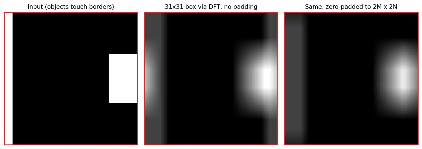
where the indices $x - m$ and $y - n$ are taken modulo $M$ and $N$. This is circular convolution: the DFT assumes the image repeats forever, so whatever is pushed off the right edge reappears on the left.

Wraparound error and padding

Circular convolution is not what we want; it mixes the left and right borders of the image. This is wraparound error. The fix is to pad both arrays with zeros so the periods are far enough apart that the copies never touch. If $f$ is $A \times B$ and $h$ is $C \times D$, choose a padded size $P \times Q$ with

$$P \ge A + C - 1, \qquad Q \ge B + D - 1$$

When the filter is specified in the frequency domain and is the same size as the image, the usual choice is simply $P = 2M$, $Q = 2N$.

Basics of filtering in the frequency domain

Plain version. Transform the image, multiply each frequency by a number that says “keep” or “remove”, and transform back. The list of numbers is the filter.

The filtering procedure

Given an $M \times N$ image $f(x, y)$ and a filter transfer function $H(u, v)$:

1. Choose padding sizes $P = 2M$ and $Q = 2N$.
2. Form the padded image $f_p(x, y)$ of size $P \times Q$ by appending zeros (or mirrored pixels).
3. Multiply $f_p$ by $(-1)^{x+y}$ to center its transform.
4. Compute the DFT, $F(u, v)$.
5. Build a real, symmetric filter $H(u, v)$ of size $P \times Q$ with its center at $(P/2, Q/2)$, and form $G(u, v) = H(u, v)\, F(u, v)$.
6. Compute $g_p(x, y) = \operatorname{Re}\{\mathcal{F}^{-1}[G(u, v)]\}\,(-1)^{x+y}$.
7. Crop the top-left $M \times N$ region to get $g(x, y)$.

Taking the real part in step 6 only discards tiny imaginary values caused by floating-point rounding; with a real image and a symmetric real filter the exact result is real.

import numpy as np

def filter_freq(f, H_of_D):
    """Filter image f with a radially symmetric, zero-phase transfer function.
    H_of_D maps a distance array D (from the centre of the P x Q grid) to H."""
    M, N = f.shape
    P, Q = 2 * M, 2 * N                                  # 1. padding size
    fp = np.zeros((P, Q)); fp[:M, :N] = f                # 2. zero-pad
    y, x = np.mgrid[0:P, 0:Q]
    fp = fp * (-1.0) ** (x + y)                          # 3. centre the transform
    F = np.fft.fft2(fp)                                  # 4. DFT
    D = np.hypot(y - P / 2, x - Q / 2)
    G = H_of_D(D) * F                                    # 5. multiply
    gp = np.real(np.fft.ifft2(G)) * (-1.0) ** (x + y)    # 6. inverse, undo centring
    return gp[:M, :N]                                    # 7. crop

Zero padding darkens a thin band along the right and bottom borders after blurring, because the filter averages in black pixels. Padding by mirroring the image (np.pad(f, ..., mode="reflect")) avoids this, which is what the figure script for this chapter does.

Zero-phase filters

Every filter in this chapter is real and symmetric about the center. Multiplying a complex number by a real number scales its magnitude and leaves its angle alone (up to a sign), so these filters change how much of each frequency remains but never where the waves line up. Such filters are called zero-phase-shift filters. After Figure 4.3 you can see why this is a requirement: changing the phase would move edges around.

Correspondence between spatial and frequency filters

By the convolution theorem, every frequency filter $H(u, v)$ has a spatial kernel $h(x, y) = \mathcal{F}^{-1}\{H(u, v)\}$, and every spatial kernel has a transfer function. The Gaussian pair is the cleanest example. In one dimension,

$$H(u) = A\, e^{-u^2 / 2\sigma^2} \;\Leftrightarrow\; h(x) = \sqrt{2\pi}\,\sigma A\, e^{-2\pi^2 \sigma^2 x^2}$$

where $\sigma$ is the width of the Gaussian in frequency. A wide frequency Gaussian corresponds to a narrow spatial kernel and vice versa. A common practical strategy is therefore to design in the frequency domain, where “pass below 40 cycles” is easy to state, and then implement a small spatial kernel that approximates $h$.

When is the frequency route faster? Spatial convolution with a $k \times k$ kernel costs about $k^2$ multiplications per pixel. The FFT route costs a fixed amount per pixel that grows only with $\log(MN)$. For small kernels (3×3, 5×5) the spatial route wins; for kernels tens of pixels wide, the FFT route wins.

Image smoothing using lowpass frequency-domain filters

Plain version. A lowpass filter keeps the slow waves and removes the fast ones, so the image gets blurrier. The way the filter drops from “keep” to “remove” matters a lot: a sudden drop creates ripples.

Let $D(u, v)$ be the distance from the center of the $P \times Q$ frequency rectangle,

$$D(u, v) = \sqrt{(u - P/2)^2 + (v - Q/2)^2}$$

and let $D_0 > 0$ be the cutoff frequency.

Ideal lowpass filter (ILPF)

$$H(u, v) = \begin{cases} 1 & D(u, v) \le D_0 \\ 0 & D(u, v) > D_0 \end{cases}$$

It passes everything inside a circle of radius $D_0$ and nothing outside. A useful way to choose $D_0$ is by the fraction of total power it keeps: the percentage $\alpha = 100 \sum_{D \le D_0} P(u, v) / \sum_{u, v} P(u, v)$.

Butterworth lowpass filter (BLPF)

$$H(u, v) = \frac{1}{1 + [D(u, v) / D_0]^{2n}}$$

where $n$ is the order. At $D = D_0$ the filter is exactly $0.5$. Small $n$ gives a gentle roll-off; as $n \to \infty$ the BLPF approaches the ideal filter.

Gaussian lowpass filter (GLPF)

$$H(u, v) = e^{-D^2(u, v) / 2D_0^2}$$

where $D_0$ plays the role of $\sigma$. At $D = D_0$ the filter is $e^{-1/2} \approx 0.607$.

Ringing

Figure 4.5 compares the three with the same cutoff. The ideal filter produces visible ringing: ghostly copies of edges repeated outward, like ripples around a stone thrown in a pond. The reason is the box-sinc pair from earlier. A sharp cutoff in frequency corresponds to a spatial kernel with a central lobe surrounded by rings of alternating sign. Convolving an edge with that kernel draws a series of faint bright and dark echoes beside it.

The Gaussian is the opposite extreme: its spatial kernel is also Gaussian, always positive, so it can never ring. The Butterworth is in between: order 1 has no ringing, order 2 has a barely visible negative lobe, and higher orders ring more and more. Order 2 is a popular compromise between a sharp cutoff and clean results.

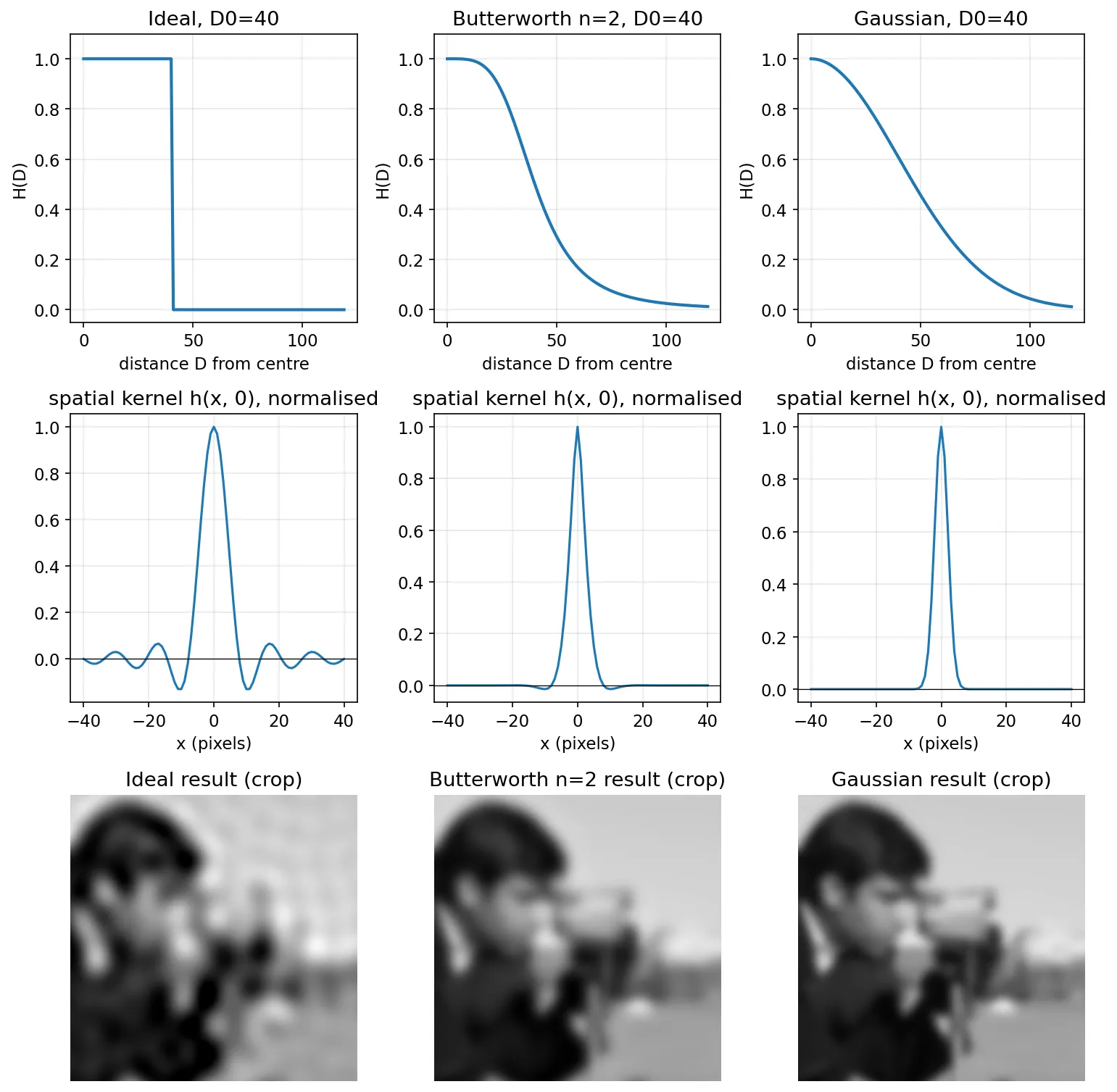
D0 = 40
ideal  = lambda D: (D <= D0).astype(float)
butter = lambda D, n=2: 1 / (1 + (D / D0) ** (2 * n))
gauss  = lambda D: np.exp(-D**2 / (2 * D0**2))
smooth = filter_freq(f, gauss)

Lowpass filtering has many quiet uses: joining broken character strokes in a low-resolution scan, softening skin texture in portraits, and suppressing scan-line patterns in remote-sensing images.

Image sharpening using highpass filters

Plain version. A highpass filter is the opposite: it throws away the slow waves and keeps the fast ones, so only edges and texture remain. Add some of that back to the original and the image looks sharper.

Ideal, Butterworth and Gaussian highpass filters

Every highpass filter can be made from a lowpass one:

$$H_{\mathrm{HP}}(u, v) = 1 - H_{\mathrm{LP}}(u, v)$$

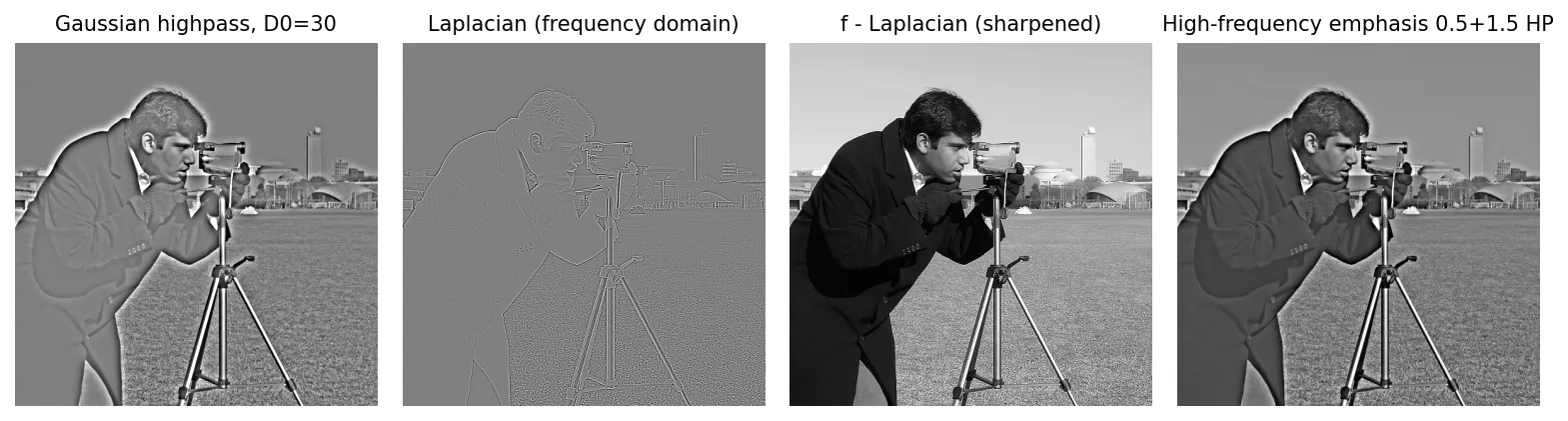
So the Gaussian highpass is $1 - e^{-D^2/2D_0^2}$, the Butterworth highpass is $1 / (1 + [D_0 / D]^{2n})$, and the ideal highpass is 0 inside the circle and 1 outside. The same ringing story applies: ideal rings, Gaussian does not. Because the highpass sets $H(0,0) = 0$, the output has zero mean, so flat regions become gray (zero) after display scaling.

The Laplacian in the frequency domain

The Laplacian $\nabla^2 f = \partial^2 f / \partial x^2 + \partial^2 f / \partial y^2$ from Chapter 3 has a transfer function. Differentiation multiplies the transform by $j 2\pi u$, so differentiating twice in each direction gives

$$H(u, v) = -4\pi^2 \left[(u - P/2)^2 + (v - Q/2)^2\right] = -4\pi^2 D^2(u, v)$$

with frequencies measured in cycles per image. The sharpened image is $g(x, y) = f(x, y) - \nabla^2 f(x, y)$, with the minus sign because the center of $H$ is negative. In practice the Laplacian output is far larger than $f$, so both must be scaled to comparable ranges (for example, $f$ in $[0, 1]$ and $\nabla^2 f$ divided by its maximum absolute value) before subtracting.

Unsharp masking, high-boost and high-frequency emphasis

Unsharp masking subtracts a blurred version to obtain a “mask” of details and adds it back:

$$g_{\mathrm{mask}}(x, y) = f(x, y) - f_{\mathrm{LP}}(x, y), \qquad g(x, y) = f(x, y) + k\, g_{\mathrm{mask}}(x, y)$$

where $f_{\mathrm{LP}}$ is a lowpass-filtered $f$ and $k \ge 0$ is a weight ($k = 1$: unsharp masking; $k > 1$: high-boost). In the frequency domain the whole operation is one transfer function, $H = 1 + k\, H_{\mathrm{HP}}$. Generalizing gives high-frequency emphasis:

$$H_{\mathrm{HFE}}(u, v) = k_1 + k_2\, H_{\mathrm{HP}}(u, v)$$

where $k_1 \ge 0$ controls how much of the low frequencies (and the DC term) survives and $k_2 \ge 0$ controls how strongly high frequencies are boosted. Choosing $k_1 < 1$ also lowers overall contrast, which is why high-frequency emphasis is often followed by histogram equalization.

Homomorphic filtering

A simple image-formation model says each pixel is the product of illumination $i(x, y)$ (how much light falls on the scene) and reflectance $r(x, y)$ (how much the surface reflects): $f = i \cdot r$. Illumination varies slowly across a scene; reflectance changes abruptly at object boundaries. We would like to squash the illumination and boost the reflectance, but the Fourier transform of a product is not the product of transforms.

The trick, introduced by Oppenheim, Schafer and Stockham [8], is to take the logarithm first, which turns the product into a sum:

$$z(x, y) = \ln f(x, y) = \ln i(x, y) + \ln r(x, y)$$

Now filter $z$ with a transfer function that treats low and high frequencies differently, and exponentiate:

$$s = \mathcal{F}^{-1}\{H\, Z\}, \qquad g(x, y) = e^{s(x, y)}, \qquad H(u, v) = (\gamma_H - \gamma_L)\left[1 - e^{-c\, D^2(u, v) / D_0^2}\right] + \gamma_L$$

where $\gamma_L \lt 1$ attenuates low frequencies (illumination), $\gamma_H > 1$ amplifies high frequencies (reflectance), $c$ controls the steepness of the transition and $D_0$ its location. The result compresses the dynamic range and enhances contrast at the same time.

def homomorphic(f, gL=0.4, gH=1.6, c=1.0, D0=30, eps=1e-3):
    z = np.log(f + eps)                       # eps avoids log(0)
    H = lambda D: (gH - gL) * (1 - np.exp(-c * D**2 / D0**2)) + gL
    return np.exp(filter_freq(z, H)) - eps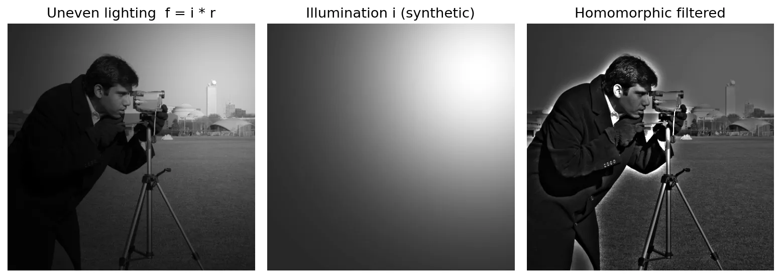

Selective filtering

Plain version. Sometimes the problem is not “too much detail” or “too little” but one specific, repeating pattern, like electrical interference stripes. In the spectrum such a pattern is a few bright dots. A selective filter removes just those dots and nothing else.

Bandreject and bandpass filters

A bandreject filter removes a ring of frequencies centered at radius $C_0$ with width $W$. The Gaussian version is

$$H_{\mathrm{BR}}(u, v) = 1 - \exp\!\left[-\left(\frac{D^2(u, v) - C_0^2}{D(u, v)\, W}\right)^{2}\right]$$

and the Butterworth version of order $n$ is

$$H_{\mathrm{BR}}(u, v) = \frac{1}{1 + \left[\dfrac{D(u, v)\, W}{D^2(u, v) - C_0^2}\right]^{2n}}$$

where $C_0$ is the ring’s center radius and $W$ its width. A bandpass filter keeps only that ring: $H_{\mathrm{BP}} = 1 - H_{\mathrm{BR}}$. Ring-shaped filters suit noise that appears at a fixed distance from the center in all directions, which is uncommon in practice.

Notch filters

A notch filter acts on small neighborhoods around chosen frequencies. Because a real image’s spectrum is conjugate symmetric, every notch must come with its mirror image through the center. A notch-reject filter with $Q$ notch pairs is built as a product of highpass filters whose centers are moved to the spike locations:

$$H_{\mathrm{NR}}(u, v) = \prod_{k=1}^{Q} H_k(u, v)\, H_{-k}(u, v)$$

where $H_k$ is a highpass filter (ideal, Butterworth or Gaussian) centered at $(u_k, v_k)$ and $H_{-k}$ is the same filter centered at $(-u_k, -v_k)$, both measured relative to the center of the frequency rectangle. The distances are

$$D_k(u, v) = \sqrt{(u - P/2 - u_k)^2 + (v - Q/2 - v_k)^2}, \qquad D_{-k}(u, v) = \sqrt{(u - P/2 + u_k)^2 + (v - Q/2 + v_k)^2}$$

A notch-pass filter is $1 - H_{\mathrm{NR}}$. Applying the notch-pass filter and inverting isolates the interference pattern itself, which is a useful check that you removed noise and not image content.

import numpy as np
from skimage import data, img_as_float

f = img_as_float(data.camera())
M, N = f.shape
y, x = np.mgrid[0:M, 0:N]
g = f + 0.2 * np.cos(2 * np.pi * (40 * x / N + 25 * y / M))   # add a ripple

G = np.fft.fftshift(np.fft.fft2(g))
u, v = y - M // 2, x - N // 2               # centred frequency coordinates
H = np.ones((M, N))
for uk, vk in [(25, 40)]:                    # spike location (row, column offset)
    for s in (+1, -1):                       # the conjugate-symmetric partner
        Dk = np.hypot(u - s * uk, v - s * vk)
        H *= 1 - np.exp(-Dk**2 / (2 * 4.0**2))   # Gaussian notch reject
out = np.real(np.fft.ifft2(np.fft.ifftshift(G * H)))

Padding is skipped here on purpose. The interference is periodic over the whole image, and padding would smear its spike across many frequency samples, making the notch less effective.

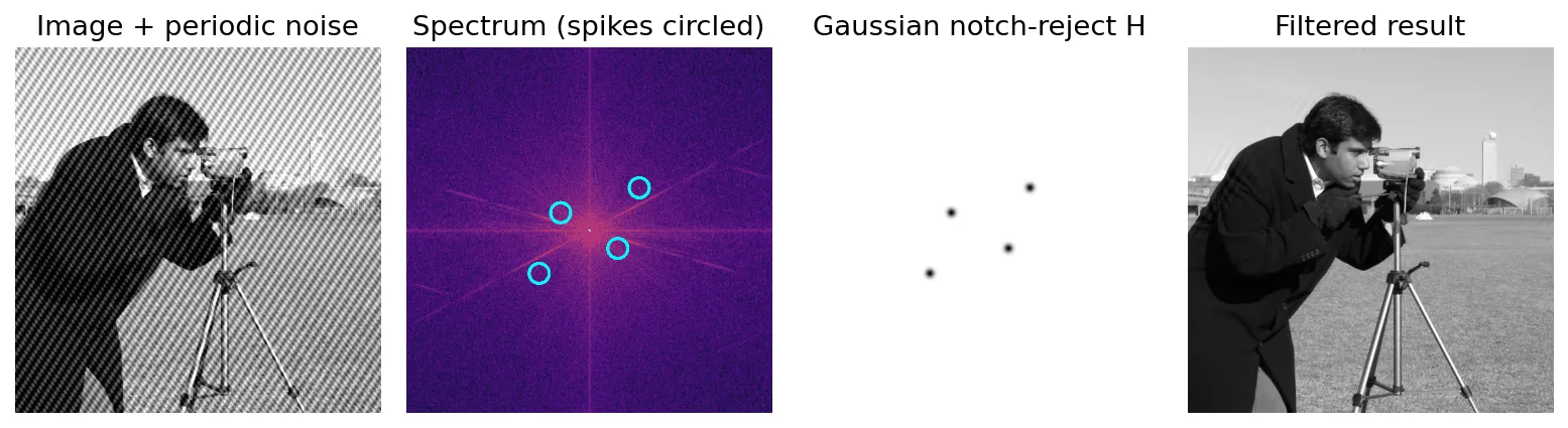
Drag the slider to compare the corrupted and filtered images directly:

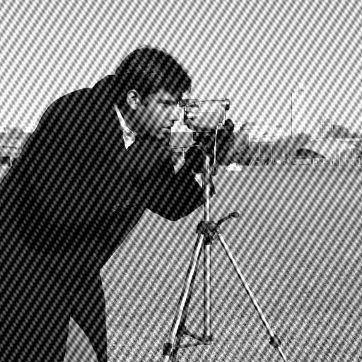
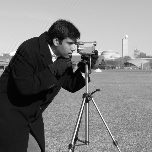With periodic noiseNotch filtered

Implementation

Plain version. A 2-D DFT can be computed as many 1-D DFTs, an inverse DFT can be computed with the forward routine, and the FFT algorithm makes each 1-D transform dramatically faster.

Separability

The 2-D kernel $e^{-j 2\pi(ux/M + vy/N)}$ factors into $e^{-j 2\pi ux/M}\, e^{-j 2\pi vy/N}$. So

$$F(u, v) = \sum_{x=0}^{M-1} e^{-j 2\pi ux/M} \underbrace{\sum_{y=0}^{N-1} f(x, y)\, e^{-j 2\pi vy/N}}_{F(x,\, v)}$$

where $F(x, v)$ is the 1-D DFT of row $x$. Compute a 1-D DFT along every row, then a 1-D DFT along every column of the result. Any 1-D FFT routine is enough to build a 2-D one.

Computing the inverse DFT with a forward transform

Take the complex conjugate of the inverse formula and multiply by $MN$:

$$MN\, f^*(x, y) = \sum_{u=0}^{M-1}\sum_{v=0}^{N-1} F^*(u, v)\, e^{-j 2\pi\left(\frac{ux}{M} + \frac{vy}{N}\right)}$$

The right side is a forward DFT of $F^*$. So: conjugate $F$, apply the forward transform, divide by $MN$ and conjugate again. For real images the final conjugation is unnecessary.

import numpy as np
F = np.fft.fft2(np.random.default_rng(1).random((8, 8)))
f_back = np.conj(np.fft.fft2(np.conj(F))) / F.size
print(np.allclose(f_back, np.fft.ifft2(F)))   # True

The fast Fourier transform

Computing the 1-D DFT from its definition takes about $M^2$ complex multiplications and additions: $M$ outputs, each a sum of $M$ terms. The FFT of Cooley and Tukey [4] reduces this to about $M \log_2 M$ for $M$ a power of 2. The core idea is divide and conquer: split the sum into even- and odd-indexed samples,

$$F(u) = F_{\mathrm{even}}(u) + W_M^{u}\, F_{\mathrm{odd}}(u), \qquad F(u + M/2) = F_{\mathrm{even}}(u) - W_M^{u}\, F_{\mathrm{odd}}(u)$$

where $W_M = e^{-j 2\pi / M}$, and $F_{\mathrm{even}}$, $F_{\mathrm{odd}}$ are DFTs of length $M/2$. Each half-length DFT is split again, until the pieces have length 1. There are $\log_2 M$ levels, each costing on the order of $M$ operations.

The ratio of the two costs, $M^2 / (M \log_2 M) = M / \log_2 M$, grows quickly. For $M = 1024$ it is about 100; for a $1024 \times 1024$ image transformed directly in 2-D (cost $(MN)^2$) versus by FFT (cost $MN \log_2 MN$), the ratio is about 50,000. On a laptop the difference is easy to see:

import time
x = np.random.default_rng(2).standard_normal(4096)
t0 = time.perf_counter(); dft(x); t1 = time.perf_counter(); np.fft.fft(x); t2 = time.perf_counter()
print(f"direct {t1 - t0:.3f}s  fft {t2 - t1:.5f}s")   # e.g. ~0.7 s vs ~0.2 ms

Modern libraries go much further than the textbook radix-2 algorithm. FFTW, described by Frigo and Johnson [6], handles arbitrary sizes, chooses among many algorithms at run time by measuring which is fastest on the actual machine, and generates its small “codelet” kernels automatically. In practice, sizes whose prime factors are small (2, 3, 5, 7) are fast; large primes are slower. scipy.fft.next_fast_len returns a good padded size.

Modern view

The Fourier transform is older than every other tool in this series, and it has aged unusually well. Deep learning did not replace it. Instead, Fourier ideas returned in three roles: a way to compute convolutions, a way to build layers with global reach, and a lens for understanding what networks learn and where they fail.

Surveys and reviews worth reading

• Unser, “Sampling — 50 years after Shannon” [3]. A review of sampling theory from Shannon’s band-limited model to modern spline and shift-invariant-space formulations. Main takeaway: the ideal sinc interpolator is a mathematical idealization; practical systems use compact kernels plus a matching prefilter, and the approximation error can be analyzed precisely in the Fourier domain. It is the best bridge from this chapter’s sampling theorem to real resampling code.
• Heideman, Johnson and Burrus, “Gauss and the history of the fast Fourier transform” [5]. A historical review tracing FFT-style algorithms back to Gauss’s unpublished work around 1805 and through many rediscoveries before 1965. Main takeaway: the algorithmic idea is simple and was found many times; what changed in 1965 was that digital computers made it matter.
• Xu, Zhang and Luo, “Overview frequency principle/spectral bias in deep learning” [13]. A survey of the frequency principle: neural networks trained by gradient descent tend to fit low-frequency components of the target first and high-frequency components later. It collects the theory and experiments behind the phenomenon and its use in algorithm design. Main takeaway: a neural network behaves, during training, a little like a lowpass filter that slowly opens up.
• Kovachki et al., “Neural Operator: Learning Maps Between Function Spaces” [15]. A long, comprehensive treatment of neural operators, which learn mappings between functions rather than between fixed-size arrays. Fourier neural operators are one of its four main parameterizations. Main takeaway: parameterizing a layer by its frequency response makes it largely independent of the grid resolution, a direct descendant of this chapter’s “filter = multiply in frequency” idea.

Fourier transforms as a fast convolution engine

The convolution theorem promises that large convolutions become cheap products. Mathieu, Henaff and LeCun [9] applied this to convolutional networks: they computed convolutions as pointwise products of FFTs on the GPU, reusing each transformed feature map many times, and reported large speedups for training. Today most CNNs use small 3×3 kernels, where direct spatial convolution usually wins, so FFT convolution is mainly used for large kernels. The reasoning in the “Correspondence between spatial and frequency filters” section above applies unchanged.

Fourier layers with a global receptive field

A pointwise product in frequency affects every pixel, so a single Fourier layer has an image-wide receptive field. Several architectures exploit this. Fast Fourier Convolution [10] adds a global branch that operates directly on the image-level spectrum, mixing global context into every layer. Global Filter Networks [11] replace the self-attention of a vision transformer with exactly the procedure from this chapter: a 2-D FFT, an element-wise product with a learned global filter, and an inverse FFT, with log-linear cost in the number of tokens. The Fourier Neural Operator [14] uses learned filters on a truncated set of low frequencies to solve partial differential equations, and because the weights live in frequency space the trained model can be evaluated on finer grids than it was trained on. These are, quite literally, learned frequency-domain filters.

A related line works on transform coefficients directly. Xu et al. [16] feed networks with the block discrete cosine transform (DCT) coefficients that common lossy image codecs already compute, and learn which frequency channels to keep. They found that many high-frequency channels can be dropped with little accuracy loss, which is consistent with the frequency principle.

Spectral bias

Rahaman et al. [12] showed that deep ReLU networks are biased towards learning low-frequency functions: high-frequency components are learned later and are less robust. Together with the overview in [13], this gives a useful mental model. A network is good at the “bass” of a target function and needs more training, data, or special input encodings to get the “cymbals” right. This explains, for example, why coordinate-based networks often struggle to represent fine textures unless their input coordinates are first mapped through sinusoidal Fourier features [20].

Aliasing comes back in deep networks

Strided convolutions and pooling are subsampling, and subsampling without a lowpass prefilter aliases, just as in Figure 4.1. Zhang [17] showed that standard CNNs are surprisingly sensitive to one-pixel shifts for this reason, and that inserting a small blur before each downsampling step (the textbook anti-aliasing filter) improves shift-invariance and, in his experiments, also image-classification accuracy. Karras et al. [18] traced an effect in which fine details of generated images appear glued to pixel coordinates, instead of moving with the depicted surfaces, to aliasing inside the generator. Their alias-free design treats feature maps as sampled continuous signals and applies carefully designed lowpass filters around every nonlinearity and resampling step.

Frequency artifacts as fingerprints

Generators upsample, and upsampling without proper interpolation filters leaves periodic patterns in the spectrum, much like the spikes in Figure 4.8. Frank et al. [19] found that GAN-generated images show strong, consistent artifacts in the frequency domain, traced them to upsampling, and used them to build a simple and accurate detector. The broader lesson is that looking at the spectrum, the oldest diagnostic in this chapter, remains one of the quickest ways to see what a generative model is doing wrong.

What did not change

Deep learning has not replaced classical frequency filtering for well-understood problems. Removing known periodic interference, anti-aliasing before resizing, fast large-kernel blurs, and homomorphic illumination correction are still done with the explicit filters in this chapter, because they are exact, fast, and need no training data. What changed is that these same ideas are now built into network architectures and used to explain their behavior.

Key takeaways

• The Fourier transform rewrites a signal as a sum of waves. Low frequencies carry smooth structure; high frequencies carry edges, texture and noise.
• Sampling copies the spectrum periodically. Sample faster than twice the highest frequency (the Nyquist rate), or blur first, otherwise aliasing and moiré appear and cannot be undone.
• The DFT treats the image as periodic. That gives circular convolution, so pad to at least $A + C - 1$ (typically $2M \times 2N$) to avoid wraparound error.
• Translation changes only the phase; rotation rotates the spectrum; real images have conjugate-symmetric spectra; and the phase carries most of the recognizable structure.
• Filtering is “transform, multiply by a real symmetric $H$, invert, crop”. Sharp cutoffs cause ringing; Gaussian filters do not; Butterworth sits in between.
• Highpass, Laplacian, high-frequency emphasis and homomorphic filters sharpen or rebalance lighting; notch filters remove periodic interference precisely.
• The FFT lowers the cost from $O(M^2)$ to $O(M \log M)$ per 1-D transform, and separability builds 2-D transforms from 1-D ones.
• In deep learning, Fourier ideas power fast convolution, global filter layers and neural operators, and explain spectral bias, aliasing in CNNs and GAN artifacts.

Exercises

1. A 1-D signal contains components at 3, 7 and 12 cycles per meter. You sample it every 0.1 m. Which components survive correctly, and at what frequency does each aliased component appear?

Hint

The sampling rate is 10 samples per meter, so the Nyquist limit is 5 cycles per meter. The 3 cycle component is fine. Fold the others back into $[-5, 5]$ by subtracting multiples of 10: 7 appears as $7 - 10 = -3$, i.e. 3 cycles per meter, and 12 appears as $12 - 10 = 2$ cycles per meter. The 7 cycle component is now indistinguishable from the real 3 cycle one.

2. Show that if $f(x, y)$ is real and symmetric, $f(x, y) = f(-x, -y)$ (indices modulo $M$, $N$), then its DFT is real. Verify numerically with a symmetric array in NumPy.

Hint

Conjugate symmetry gives $F(-u,-v) = F^*(u,v)$ for any real $f$. Symmetry of $f$ gives $F(-u,-v) = F(u,v)$ by substituting $x \to -x$, $y \to -y$ in the definition. Together, $F = F^*$, so $F$ is real. For the check, build g = a + np.roll(a[::-1, ::-1], 1, axis=(0, 1)) for a random a and confirm np.abs(np.fft.fft2(g).imag).max() is near zero.

3. Using the filter_freq function, filter the camera image with a Butterworth lowpass filter of orders 1, 2, 5 and 20 at $D_0 = 30$. At what order does ringing first become clearly visible? Plot the central row of each filter’s spatial kernel and relate it to what you see.

Hint

Obtain the kernel by inverse-transforming the centered filter and shifting it back to the center. Ringing appears when the kernel develops noticeable negative side lobes. Order 1 has none, order 2 has a tiny one, and by order 5 to 20 the lobes approach those of the ideal filter.

4. You filter a 300 × 400 image with a 51 × 51 spatial kernel using FFTs. What is the minimum padded size that avoids wraparound error? Would you choose that size or a slightly larger one, and why?

Hint

The minimum is $(300 + 51 - 1) \times (400 + 51 - 1) = 350 \times 450$. Both are fine, but sizes with only small prime factors are faster for FFT libraries. $350 = 2 \cdot 5^2 \cdot 7$ and $450 = 2 \cdot 3^2 \cdot 5^2$ already are, so they are good choices; scipy.fft.next_fast_len confirms this.

5. Photograph (or synthesize) an image with two different periodic interference patterns. Design a notch-reject filter that removes only one of them, then use the corresponding notch-pass filter to display the pattern you removed. How do you choose the notch radius?

Hint

Locate the spikes in the log spectrum, ignoring the DC peak and the axes. Remember each spike’s mirror twin. A radius just large enough to cover the spike’s spread works best: too small leaves residual stripes, too large removes image content near those frequencies. The notch-pass output should look like clean stripes with no trace of the scene.

6. Explain, using the ideas in this chapter, why inserting a blur before every stride-2 layer can make a CNN’s output more stable when the input image is shifted by one pixel.

Hint

Stride-2 subsampling halves the sampling rate, so frequencies above the new Nyquist limit fold back as aliases. A one-pixel shift changes the phase of those components, and after aliasing that changes the low-frequency output, so the next layers see a different signal. A lowpass filter removes those frequencies first, so a shift changes the output much less. See [17].

References

1. R. C. Gonzalez and R. E. Woods, Digital Image Processing, 4th ed., Pearson, 2018, Ch. 4. publisher page
2. C. E. Shannon, “Communication in the presence of noise,” Proceedings of the IRE, vol. 37, no. 1, pp. 10–21, 1949. doi
3. M. Unser, “Sampling—50 years after Shannon,” Proceedings of the IEEE, vol. 88, no. 4, pp. 569–587, 2000. doi
4. J. W. Cooley and J. W. Tukey, “An algorithm for the machine calculation of complex Fourier series,” Mathematics of Computation, vol. 19, no. 90, 1965. doi
5. M. T. Heideman, D. H. Johnson and C. S. Burrus, “Gauss and the history of the fast Fourier transform,” IEEE ASSP Magazine, vol. 1, no. 4, pp. 14–21, 1984. doi
6. M. Frigo and S. G. Johnson, “The design and implementation of FFTW3,” Proceedings of the IEEE, vol. 93, no. 2, 2005. doi
7. A. V. Oppenheim and J. S. Lim, “The importance of phase in signals,” Proceedings of the IEEE, vol. 69, no. 5, 1981. doi
8. A. V. Oppenheim, R. W. Schafer and T. G. Stockham, “Nonlinear filtering of multiplied and convolved signals,” Proceedings of the IEEE, vol. 56, no. 8, pp. 1264–1291, 1968. doi
9. M. Mathieu, M. Henaff and Y. LeCun, “Fast training of convolutional networks through FFTs,” arXiv:1312.5851, 2013. arXiv
10. L. Chi, B. Jiang and Y. Mu, “Fast Fourier convolution,” Advances in Neural Information Processing Systems (NeurIPS), vol. 33, 2020. proceedings
11. Y. Rao, W. Zhao, Z. Zhu, J. Lu and J. Zhou, “Global filter networks for image classification,” NeurIPS, 2021. arXiv
12. N. Rahaman, A. Baratin, D. Arpit, F. Draxler, M. Lin, F. A. Hamprecht, Y. Bengio and A. Courville, “On the spectral bias of neural networks,” ICML, 2019. arXiv
13. Z.-Q. J. Xu, Y. Zhang and T. Luo, “Overview frequency principle/spectral bias in deep learning,” arXiv:2201.07395, 2022. arXiv
14. Z. Li, N. Kovachki, K. Azizzadenesheli, B. Liu, K. Bhattacharya, A. Stuart and A. Anandkumar, “Fourier neural operator for parametric partial differential equations,” arXiv:2010.08895, 2020. arXiv
15. N. Kovachki, Z. Li, B. Liu, K. Azizzadenesheli, K. Bhattacharya, A. Stuart and A. Anandkumar, “Neural operator: Learning maps between function spaces,” Journal of Machine Learning Research, vol. 24, 2023. arXiv
16. K. Xu, M. Qin, F. Sun, Y. Wang, Y.-K. Chen and F. Ren, “Learning in the frequency domain,” CVPR, 2020. arXiv
17. R. Zhang, “Making convolutional networks shift-invariant again,” ICML, 2019. arXiv
18. T. Karras, M. Aittala, S. Laine, E. Härkönen, J. Hellsten, J. Lehtinen and T. Aila, “Alias-free generative adversarial networks,” arXiv:2106.12423, 2021. arXiv
19. J. Frank, T. Eisenhofer, L. Schönherr, A. Fischer, D. Kolossa and T. Holz, “Leveraging frequency analysis for deep fake image recognition,” ICML, 2020. arXiv
20. M. Tancik, P. P. Srinivasan, B. Mildenhall, S. Fridovich-Keil, N. Raghavan, U. Singhal, R. Ramamoorthi, J. T. Barron and R. Ng, “Fourier features let networks learn high frequency functions in low dimensional domains,” arXiv:2006.10739, 2020. arXiv