Chapter 11 · Image Segmentation II: Active Contours — Snakes and Level Sets

What you’ll learn

• Why segmentation can be posed as moving a curve until an energy stops decreasing, and what that buys over thresholding and edge linking.
• How a snake (an explicit, parametric active contour) is defined by internal and external energies, and how the Euler–Lagrange equation turns that energy into an iterative algorithm.
• How to pick the external force: image gradients, edge maps, gradient vector flow (GVF) and the balloon force, and why each one exists.
• How the level-set method represents a curve implicitly as the zero crossing of a function $\phi$, and how to evolve it with $\phi_t + F\lvert\nabla\phi\rvert = 0$ using upwind finite differences under a CFL limit.
• How the speed function encodes edge-based (geodesic active contours) and region-based (Chan–Vese, from Mumford–Shah) models, plus signed-distance reinitialization, narrow bands and morphological approximations.
• Where active contours live today: inside deep networks as contour-refinement heads and as loss functions.

The big picture

Chapter 10 segmented images with local rules: threshold this pixel, link that edge, grow this region. Those rules know nothing about the shape of what they produce. The result can be a boundary with gaps, a region that leaks through a weak edge, or a speckle of isolated pixels.

Active contours take a different view. We start with a closed curve somewhere near the object and let it move. The curve is pushed by the image (toward edges, or toward a good split into “inside” and “outside”) and held together by its own stiffness (it resists stretching and bending). When the pushes and the stiffness balance, the curve stops, and its final position is the segmentation. The output is always a closed, smooth boundary, never a heap of edge fragments.

Following the textbook [1], this chapter covers the two families in that order. Snakes (Kass, Witkin and Terzopoulos [2]) store the curve as a list of points and move the points directly. Level sets (Osher and Sethian [5]) store the curve implicitly as the zero contour of a surface and move the surface instead, which makes splitting and merging automatic. Both are variational: we write down an energy, then do gradient descent on it. That idea, more than any particular formula, is what survived into deep learning.

Background: why curves that move

In plain words: instead of deciding pixel by pixel, we describe the whole boundary at once and ask, “how good is this boundary?” Then we improve it a little at a time.

More precisely, an active contour method has three ingredients:

1. A representation of a closed curve $C$ in the image domain $\Omega \subset \mathbb{R}^2$: either explicit (a parametrized curve $v(s)$) or implicit (the zero level set of a function $\phi(x, y)$).
2. An energy $E(C)$ that is low when $C$ is a good boundary. It always mixes a regularity term (short, smooth curves are preferred) with a data term (edges are strong along the curve, or the regions inside and outside are each homogeneous).
3. An evolution rule that changes $C$ to decrease $E$, usually gradient descent written as a partial differential equation (PDE) in an artificial time $t$.

Compared with Chapter 10, the regularity term bridges gaps in edges, the output is always a closed curve ready for the shape descriptors of Chapter 12, and prior knowledge (a user’s click, a smoothness preference, an intensity model) enters naturally.

The price is that the energy is non-convex: gradient descent finds a local minimum, so the answer depends on where you start.

Image segmentation using snakes

A snake is a closed chain of points that slides over the image. Each point feels two kinds of pull: its neighbours keep the chain short and smooth, and the image drags it toward edges.

The snake as a parametric curve

We write the contour as

$$v(s) = \big(x(s),\, y(s)\big), \qquad s \in [0, 1], \quad v(0) = v(1),$$

where $s$ is a parameter that runs once around the curve and $x(s)$, $y(s)$ are image coordinates. Derivatives with respect to $s$ are written $v_s = dv/ds$ and $v_{ss} = d^2 v / ds^2$. In a computer the curve is sampled at $n$ points $v_i = (x_i, y_i)$, $i = 0, \dots, n-1$, with indices taken modulo $n$ for a closed snake.

The energy functional

The snake energy of [2] is

$$E_{\text{snake}}(v) = \int_0^1 \Big[\, \underbrace{\tfrac12\big(\alpha\,\lvert v_s(s)\rvert^2 + \beta\,\lvert v_{ss}(s)\rvert^2\big)}_{E_{\text{int}}} \;+\; E_{\text{ext}}\big(v(s)\big) \Big]\, ds .$$

• $\alpha \ge 0$ is the elasticity (tension) weight. The term $\lvert v_s\rvert^2$ is large when the curve is stretched, so $\alpha$ makes the snake behave like an elastic string that wants to shrink.
• $\beta \ge 0$ is the rigidity (bending) weight. The term $\lvert v_{ss}\rvert^2$ measures how sharply the curve turns, so $\beta$ makes the snake behave like a thin metal rod that resists kinks.
• $E_{\text{ext}}(x, y)$ is the external (image) energy, a scalar field over the image that is low where we want the snake to settle.

A common choice of external energy for a gray-level image $f$ is

$$E_{\text{ext}}(x, y) = -\,w_{\text{edge}}\,\big\lvert \nabla\big(G_\sigma * f\big)(x, y)\big\rvert^2 \;-\; w_{\text{line}}\,(G_\sigma * f)(x, y),$$

where $G_\sigma$ is a Gaussian of standard deviation $\sigma$, $*$ is convolution, $\nabla$ is the gradient, and $w_{\text{edge}}$, $w_{\text{line}}$ are weights. With $w_{\text{edge}} > 0$ the snake is attracted to strong edges. With $w_{\text{line}} > 0$ it is attracted to dark lines, and with $w_{\text{line}} \lt 0$ to bright lines. The Gaussian blur widens the valleys of $E_{\text{ext}}$ so that the snake can feel an edge from a few pixels away; [2] calls this scale-space continuation.

From energy to motion: the Euler–Lagrange equation

To minimize an integral of the form $\int L(v, v_s, v_{ss})\,ds$ we use the calculus of variations. A minimizer must satisfy the Euler–Lagrange equation

$$\frac{\partial L}{\partial v} - \frac{d}{ds}\frac{\partial L}{\partial v_s} + \frac{d^2}{ds^2}\frac{\partial L}{\partial v_{ss}} = 0 .$$

With $L = \tfrac12\alpha\lvert v_s\rvert^2 + \tfrac12\beta\lvert v_{ss}\rvert^2 + E_{\text{ext}}(v)$ we have $\partial L/\partial v = \nabla E_{\text{ext}}$, $\partial L/\partial v_s = \alpha v_s$ and $\partial L/\partial v_{ss} = \beta v_{ss}$. For constant $\alpha$ and $\beta$ this gives

$$\alpha\, v_{ss} - \beta\, v_{ssss} - \nabla E_{\text{ext}}(v) = 0 .$$

Read it as a force balance. $\alpha v_{ss}$ is the tension force (it points toward the local centre of curvature and shortens the curve), $-\beta v_{ssss}$ is the bending force (it straightens kinks), and $F_{\text{ext}} = -\nabla E_{\text{ext}}$ is the image force. At equilibrium they cancel.

We rarely can solve this equation directly, so we make $v$ depend on an artificial time $t$ and let it slide downhill:

$$\gamma\, \frac{\partial v}{\partial t} = \alpha\, v_{ss} - \beta\, v_{ssss} + F_{\text{ext}}(v),$$

where $\gamma > 0$ is a viscosity (damping) constant. When $\partial v/\partial t = 0$ we are back at the Euler–Lagrange equation.

Discretization and the iterative solution

Sample the curve at $n$ points with unit spacing. Central differences give

$$v_{ss} \approx v_{i+1} - 2v_i + v_{i-1}, \qquad v_{ssss} \approx v_{i+2} - 4v_{i+1} + 6v_i - 4v_{i-1} + v_{i-2}.$$

Stack the $x$ coordinates into a vector $\mathbf{x} \in \mathbb{R}^n$ (and likewise $\mathbf{y}$). Then $\alpha v_{ss} - \beta v_{ssss} = -A\mathbf{x}$, where $A$ is a symmetric, circulant, pentadiagonal $n\times n$ matrix whose rows contain

$$\big[\;\beta,\;\; -\alpha - 4\beta,\;\; 2\alpha + 6\beta,\;\; -\alpha - 4\beta,\;\; \beta\;\big]$$

centred on the diagonal (wrapping around at the ends). The internal forces are linear in the point positions; the external force is not. The classic trick of [2] is a semi-implicit step: treat the internal part implicitly (at the new time $t$) and the external part explicitly (at the old time $t-1$):

$$\gamma\,(\mathbf{x}^{t} - \mathbf{x}^{t-1}) = -A\,\mathbf{x}^{t} + \mathbf{f}_x\big(\mathbf{x}^{t-1}, \mathbf{y}^{t-1}\big) \;\;\Longrightarrow\;\; \mathbf{x}^{t} = (A + \gamma I)^{-1}\big(\gamma\,\mathbf{x}^{t-1} + \mathbf{f}_x\big),$$

and the same for $\mathbf{y}$ with $\mathbf{f}_y$. Here $\mathbf{f}_x$, $\mathbf{f}_y$ are the components of $F_{\text{ext}}$ sampled (by interpolation) at the current points, and $I$ is the identity. The matrix $(A + \gamma I)$ is fixed, so it is inverted or factorized once; each iteration is then a cheap matrix–vector product. The implicit treatment of the stiff fourth-order term is what lets the snake take reasonable steps without blowing up. The step size is $1/\gamma$: a larger $\gamma$ means smaller, safer steps.

import numpy as np

def snake_step_matrix(n, alpha, beta, gamma):
    """(A + gamma*I)^-1 for a closed snake with n points (h = 1)."""
    row = np.zeros(n)
    row[[0, 1, 2, -2, -1]] = [2*alpha + 6*beta, -alpha - 4*beta, beta,
                              beta, -alpha - 4*beta]
    A = np.stack([np.roll(row, i) for i in range(n)])
    return np.linalg.inv(A + gamma * np.eye(n))

M = snake_step_matrix(100, alpha=0.05, beta=0.05, gamma=1.0)
# one iteration, given external forces fx, fy sampled at the points:
# x = M @ (gamma * x + fx);  y = M @ (gamma * y + fy)

scikit-image’s active_contour implements exactly this scheme, with the edge and line energies above and an extra cap on how far a point may move per iteration [12]:

import numpy as np
from skimage import data
from skimage.color import rgb2gray
from skimage.filters import gaussian
from skimage.segmentation import active_contour

img = rgb2gray(data.astronaut())
s = np.linspace(0, 2 * np.pi, 400)
init = np.column_stack([100 + 100 * np.sin(s),   # rows
                        220 + 100 * np.cos(s)])  # columns
snake = active_contour(gaussian(img, sigma=3), init,
                       alpha=0.015, beta=10, gamma=0.001)
print(snake.shape)  # (400, 2): the final (row, col) points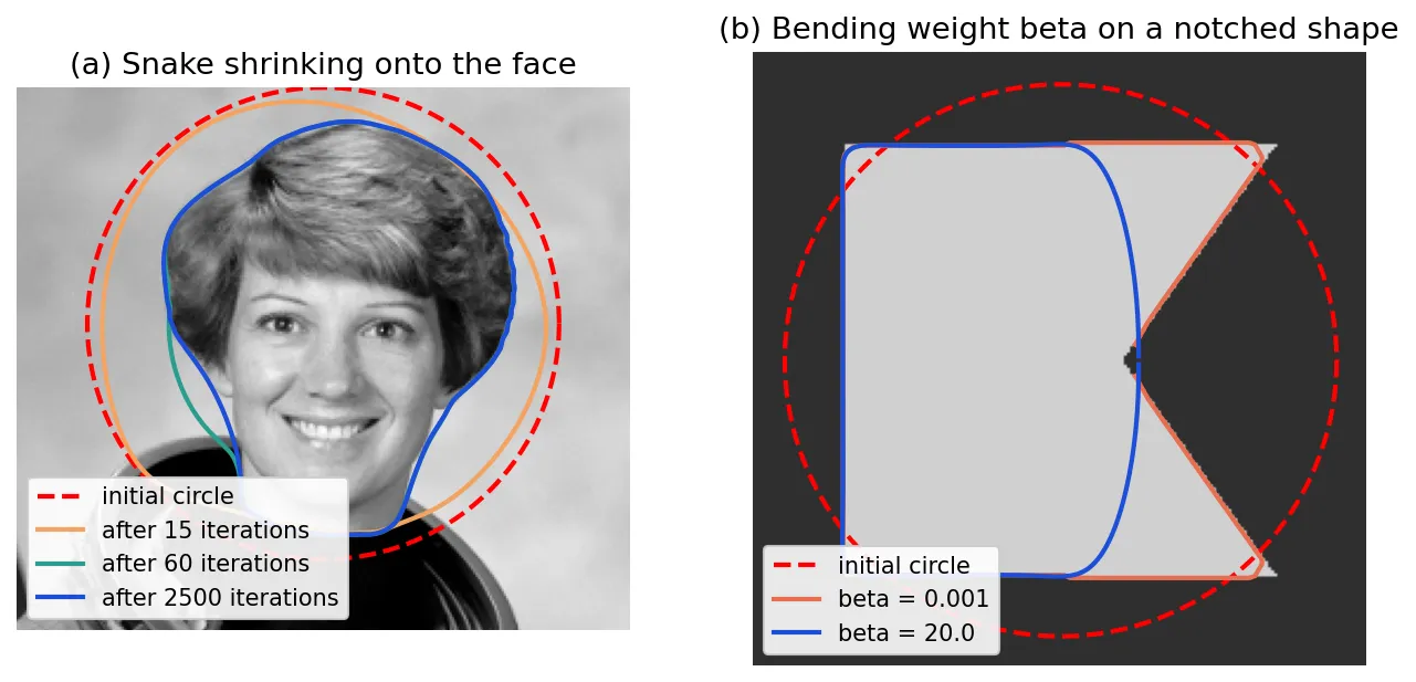

Figure 11.1(a) shows the typical life of a snake: it shrinks quickly through the flat background (tension alone), then slows as it enters the zone where the blurred edge map has a slope, and finally locks onto the strongest nearby edges. Panel (b) shows the trade-off that $\beta$ controls. A stiff snake is robust to noise and small gaps, but it cannot follow corners or concavities.

Choosing the external force

The external force decides what the snake looks for. Common choices:

• Gradient of an edge map. Compute an edge map $e(x, y) \ge 0$ that is large on edges, for example $e = \lvert\nabla(G_\sigma * f)\rvert$ (or its square), and use $F_{\text{ext}} = \kappa\, \nabla e$ with a weight $\kappa$. The force points uphill on $e$, toward the ridge of the edge.
• Line attraction. Use $F_{\text{ext}} = \pm\nabla (G_\sigma * f)$ to follow dark or bright curvilinear structures (roads, vessels, text strokes).

All of them share the same weakness. The gradient of an edge map is essentially zero away from edges (Figure 11.2a). A snake that starts far from the boundary feels nothing but its own tension. And inside a narrow concavity the forces from the two walls point sideways and cancel, so nothing pulls the snake down into it. These two problems, limited capture range and poor convergence into concavities, motivated GVF.

Gradient vector flow (GVF)

GVF keeps the good part of $\nabla e$ (accurate, pointing at edges where edges exist) and fills in the rest of the image by smooth diffusion. Xu and Prince [3] define the GVF field $\mathbf{w}(x, y) = (u(x, y), v(x, y))$ as the minimizer of

$$\mathcal{E}(\mathbf{w}) = \iint_\Omega \mu\,\big(u_x^2 + u_y^2 + v_x^2 + v_y^2\big) \;+\; \lvert\nabla e\rvert^2\,\lvert \mathbf{w} - \nabla e\rvert^2 \; dx\,dy .$$

• $u_x, u_y, v_x, v_y$ are the partial derivatives of the two field components; the first term asks the field to vary slowly.
• $\lvert\nabla e\rvert^2\,\lvert\mathbf{w} - \nabla e\rvert^2$ asks $\mathbf{w}$ to equal $\nabla e$, but only where $\lvert\nabla e\rvert$ is large, that is, near edges.
• $\mu > 0$ balances the two; it should grow with the noise level.

The Euler–Lagrange equations are a pair of decoupled diffusion equations. Solving them by gradient descent in time gives

$$u_t = \mu\,\nabla^2 u - (u - e_x)\,\lvert\nabla e\rvert^2, \qquad v_t = \mu\,\nabla^2 v - (v - e_y)\,\lvert\nabla e\rvert^2,$$

where $\nabla^2$ is the Laplacian and $e_x$, $e_y$ are the components of $\nabla e$. Far from edges the second term vanishes and the field simply diffuses outward from the edges, carrying their direction with it. With unit time step and the 5-point Laplacian, the explicit scheme is stable for $\mu \le 1/4$ when $e$ is scaled to $[0, 1]$.

import numpy as np
from scipy import ndimage as ndi

def gvf(f, mu=0.2, iters=500):
    """Gradient vector flow of an edge map f scaled to [0, 1]."""
    fy, fx = np.gradient(f)
    mag2 = fx**2 + fy**2
    u, v = fx.copy(), fy.copy()
    for _ in range(iters):  # explicit scheme, stable for mu <= 0.25
        u += mu * ndi.laplace(u, mode="nearest") - (u - fx) * mag2
        v += mu * ndi.laplace(v, mode="nearest") - (v - fy) * mag2
    return u, v

The snake then uses $F_{\text{ext}} = \kappa\,\mathbf{w}$ in place of $\kappa\,\nabla e$, with no other change to the algorithm.

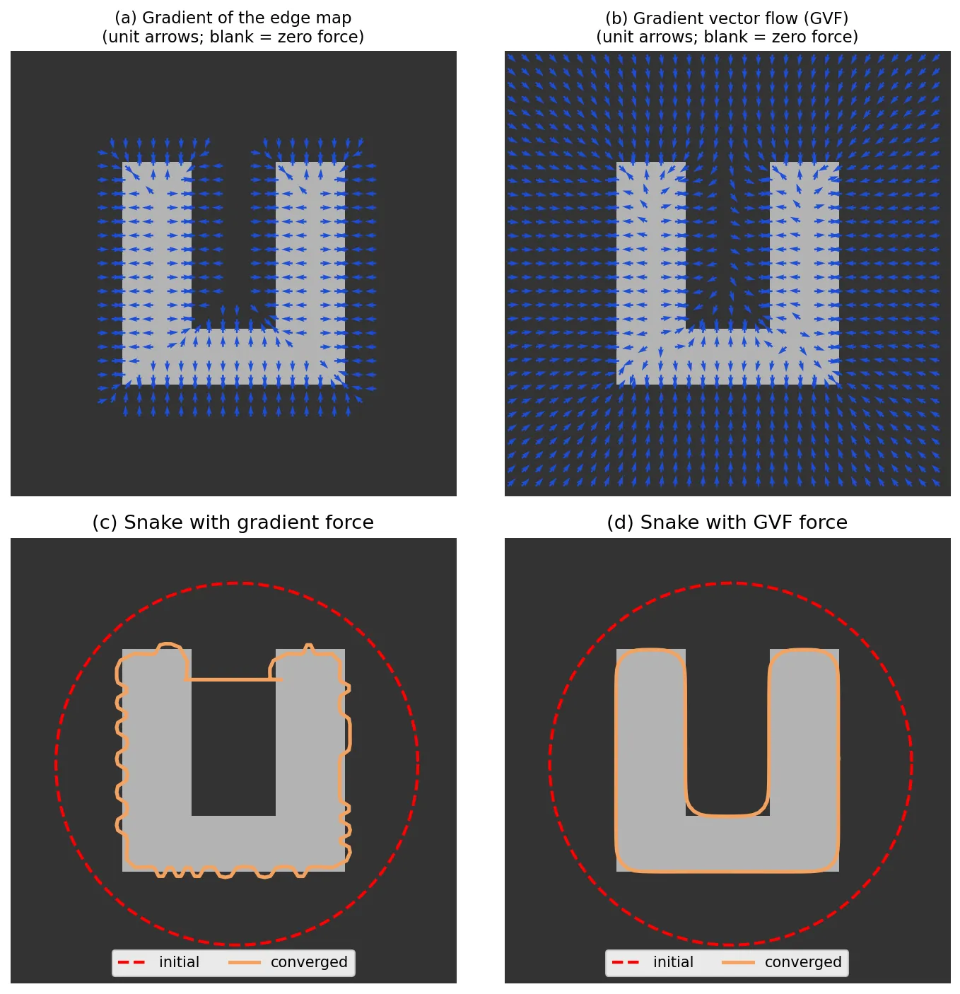
Figure 11.2 reproduces the classic test of [3] on a synthetic U shape. Two things changed: the snake now feels the object from anywhere in the image (large capture range), and inside the notch the diffused vectors point down rather than sideways, so the snake is pulled into the concavity. One implementation detail matters: as the snake enters the notch its length grows, so the points must be resampled to a roughly constant spacing every few dozen iterations, or the chain becomes too sparse to follow the walls.

The balloon force

Cohen [4] attacked the capture-range problem from another angle. If you initialize a small snake inside the object, tension makes it shrink to a point before any edge force can reach it. So add a pressure:

$$F_{\text{ext}}(v) = \kappa\,\nabla e(v) \;+\; k_1\, \mathbf{n}(s),$$

where $\mathbf{n}(s)$ is the unit outward normal of the curve at $v(s)$ and $k_1$ is the pressure. With $k_1 > 0$ the snake inflates like a balloon; with $k_1 \lt 0$ it deflates. The edge force must be able to beat the pressure at a real boundary ($\kappa\,\lvert\nabla e\rvert > \lvert k_1\rvert$ there), but not at the weak, noisy gradients inside the object. Cohen also suggests normalizing the edge force, $\nabla e/\lvert\nabla e\rvert$, so that one constant controls its strength everywhere.

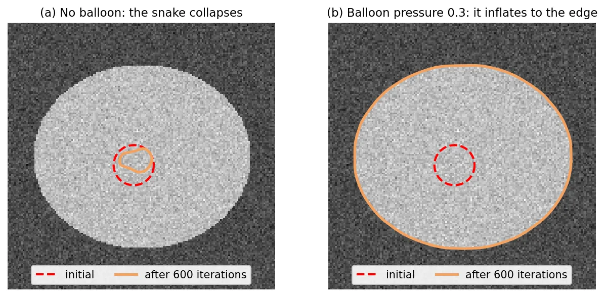
The balloon force has a cost: you must know in advance whether to inflate or deflate, and too much pressure carries the snake straight through weak edges. GVF and balloon forces are complementary and are often combined.

Limitations of snakes

• Initialization. The energy has many local minima. Even with GVF, a snake started across two objects or on the wrong side of a strong clutter edge will converge to the wrong answer.
• Parameter tuning. $\alpha$, $\beta$, $\gamma$, $\kappa$, the blur $\sigma$, the pressure $k_1$ and the GVF $\mu$ interact. Values that work on one image often fail on the next.
• Point management. The points drift along the curve, bunch up in some places and spread out in others. Practical snakes resample the curve and must detect when it crosses itself.
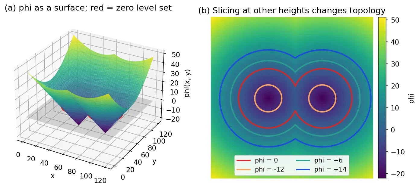
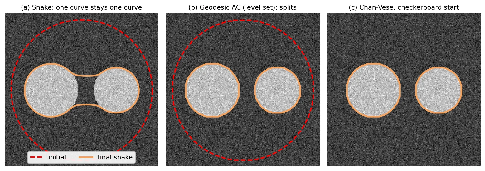
• Topology is fixed. A snake is one closed chain. It cannot split into two when it encloses two objects (Figure 11.6a), and it cannot merge with another snake, without extra, error-prone bookkeeping.

The last limitation is the one level sets remove.

Segmentation using level sets

Instead of tracking the boundary itself, track a landscape whose shoreline is the boundary. Move the landscape up or down, and the shoreline moves with it. If the water rises enough to separate two hills, the one shoreline becomes two, with no special code.

The implicit representation

A level-set function is a scalar function $\phi: \Omega \times [0, \infty) \to \mathbb{R}$ such that the curve at time $t$ is its zero level set:

$$C(t) = \{\, (x, y) \in \Omega \;:\; \phi(x, y, t) = 0 \,\}.$$

We use the convention $\phi \lt 0$ inside the curve and $\phi > 0$ outside. (Some papers, including [8], use the opposite sign; the equations change sign accordingly.) Two geometric quantities come for free from $\phi$:

$$\mathbf{N} = \frac{\nabla\phi}{\lvert\nabla\phi\rvert}, \qquad \kappa = \nabla\cdot\frac{\nabla\phi}{\lvert\nabla\phi\rvert},$$

where $\mathbf{N}$ is the unit outward normal and $\kappa$ is the curvature of the level curve through each point (positive on convex parts; for a circle of radius $r$, $\kappa = 1/r$).

The most convenient $\phi$ is the signed distance function: $\lvert\phi(x, y)\rvert$ is the Euclidean distance from $(x, y)$ to $C$, with the sign telling inside from outside. It satisfies $\lvert\nabla\phi\rvert = 1$ almost everywhere, which keeps the numerics well behaved.

The level-set equation

Suppose each point of the curve moves along its outward normal with speed $F$ (positive means outward):

$$\frac{\partial C}{\partial t} = F\,\mathbf{N}.$$

Points on the curve keep the value zero, so $\phi\big(C(t), t\big) = 0$ for all $t$. Differentiate with the chain rule:

$$\phi_t + \nabla\phi\cdot\frac{\partial C}{\partial t} = 0 \;\;\Longrightarrow\;\; \phi_t + F\,\nabla\phi\cdot\frac{\nabla\phi}{\lvert\nabla\phi\rvert} = 0 \;\;\Longrightarrow\;\; \boxed{\;\phi_t + F\,\lvert\nabla\phi\rvert = 0\;}$$

This is the level-set equation of Osher and Sethian [5]. $\phi_t$ is the time derivative of $\phi$ and $F$ is the speed function, which may depend on position (image data), on the geometry of the curve (curvature $\kappa$), or on global statistics. The equation is solved on the fixed pixel grid for all $(x, y)$, not only on the curve; the curve is read off at any time by extracting the zero contour. Nothing in the equation cares how many pieces the zero set has, which is why splitting and merging happen naturally.

Discrete computation: upwind differences and the CFL condition

Let $\phi^n_{ij}$ be the value at pixel $(i, j)$ after $n$ steps of size $\Delta t$, with grid spacing $\Delta x = 1$. The one-sided differences

$$D^{-x}_{ij} = \phi_{ij} - \phi_{i-1,j}, \qquad D^{+x}_{ij} = \phi_{i+1,j} - \phi_{ij}$$

(and $D^{\pm y}$ likewise) are combined so that information is always taken from the side the front is coming from. This is the upwind scheme of [5]:

$$\phi^{n+1}_{ij} = \phi^n_{ij} - \Delta t\,\Big[\max(F_{ij}, 0)\,\nabla^{+}_{ij} + \min(F_{ij}, 0)\,\nabla^{-}_{ij}\Big],$$ $$\nabla^{+} = \sqrt{\max(D^{-x}, 0)^2 + \min(D^{+x}, 0)^2 + \max(D^{-y}, 0)^2 + \min(D^{+y}, 0)^2},$$ $$\nabla^{-} = \sqrt{\min(D^{-x}, 0)^2 + \max(D^{+x}, 0)^2 + \min(D^{-y}, 0)^2 + \max(D^{+y}, 0)^2}.$$

Using a plain central difference here instead produces oscillations and corners that smear or explode; upwinding is what keeps the front sharp and stable.

The explicit scheme is stable only if the front moves less than one cell per step. This is the Courant–Friedrichs–Lewy (CFL) condition:

$$\Delta t \,\max_{ij}\lvert F_{ij}\rvert \le c\,\Delta x, \qquad 0 \lt c \le 1 .$$

If $F$ contains a curvature term $b\,\kappa$, that part behaves like diffusion and is discretized with central differences; it adds a stricter, second-order limit of roughly $\Delta t \le \Delta x^2 / (4b)$ in 2D. In practice you compute $\Delta t$ from the current maximum speed at each step.

import numpy as np
from scipy import ndimage as ndi

def signed_distance(mask):
    """Negative inside, positive outside, ~0 on the boundary."""
    return ndi.distance_transform_edt(~mask) - ndi.distance_transform_edt(mask)

def evolve(phi, F, steps=100, cfl=0.5):
    """Upwind scheme for phi_t + F |grad phi| = 0 (F is an array or scalar)."""
    for _ in range(steps):
        p = np.pad(phi, 1, mode="edge")
        dxm = phi - p[1:-1, :-2]; dxp = p[1:-1, 2:] - phi   # backward / forward
        dym = phi - p[:-2, 1:-1]; dyp = p[2:, 1:-1] - phi
        grad_plus = np.sqrt(np.maximum(dxm, 0)**2 + np.minimum(dxp, 0)**2 +
                            np.maximum(dym, 0)**2 + np.minimum(dyp, 0)**2)
        grad_minus = np.sqrt(np.minimum(dxm, 0)**2 + np.maximum(dxp, 0)**2 +
                             np.minimum(dym, 0)**2 + np.maximum(dyp, 0)**2)
        dt = cfl / (np.abs(F).max() + 1e-12)             # CFL: |F| dt <= dx
        phi = phi - dt * (np.maximum(F, 0) * grad_plus + np.minimum(F, 0) * grad_minus)
    return phi

yy, xx = np.mgrid[:128, :128]
phi = signed_distance((xx - 64)**2 + (yy - 64)**2 < 20**2)
phi = evolve(phi, F=1.0, steps=20)                # grow outward by 20 * 0.5 = 10 px
phi = signed_distance(phi < 0)                     # re-initialize
print(np.sqrt((phi < 0).sum() / np.pi))            # radius, about 30

Specifying the speed function

All the image analysis lives in $F$. Two families dominate.

Edge-based speed: geodesic active contours

Define an edge-stopping function that is close to $1$ in flat regions and close to $0$ on edges, for example

$$g(x, y) = \frac{1}{1 + \lvert\nabla(G_\sigma * f)(x, y)\rvert^2}.$$

Caselles, Kimmel and Sapiro [6] showed that a snake with $\beta = 0$ is closely related to finding a curve of minimal weighted length

$$L_g(C) = \oint_C g\big(C(s)\big)\, ds,$$

where $ds$ is arc length. In the metric defined by $g$, edges are “cheap” places to be, so a minimizer is a geodesic (shortest path) that hugs edges. This is the geodesic active contour (GAC). Gradient descent on $L_g$, plus an optional constant pressure $c$ like Cohen’s balloon, gives in our sign convention

$$\phi_t = g\,\lvert\nabla\phi\rvert\,(\kappa - c) + \nabla g\cdot\nabla\phi .$$

Each term has a job. $g\,\kappa\,\lvert\nabla\phi\rvert$ is curvature flow (shortening and smoothing) that slows to a stop near edges. $-c\,g\,\lvert\nabla\phi\rvert$ is the pressure: $c > 0$ inflates, $c \lt 0$ deflates, again switched off on edges. $\nabla g\cdot\nabla\phi$ is an advection term that pulls the curve into the bottom of the edge valley, where $g$ is minimal, and stops it from overshooting. Unlike a snake, the GAC is intrinsic: it does not depend on how the curve is parametrized, and in level-set form it splits and merges freely.

Because $g$ never reaches exactly zero, a strong pressure still leaks through weak or blurred edges. That is the motivation for region-based speeds.

Region-based speed: Mumford–Shah and Chan–Vese

Mumford and Shah [7] posed segmentation as finding a piecewise-smooth approximation $u$ of the image $f$ together with a set of boundaries $C$:

$$E_{\text{MS}}(u, C) = \int_\Omega (u - f)^2\, dx\,dy \;+\; \mu \int_{\Omega\setminus C} \lvert\nabla u\rvert^2\, dx\,dy \;+\; \nu\,\lvert C\rvert,$$

where the first term asks $u$ to stay close to $f$, the second asks $u$ to be smooth except across $C$, and $\lvert C\rvert$ is the total boundary length. This energy is hard to minimize in general.

Chan and Vese [8] restricted $u$ to be piecewise constant with two values: $c_1$ inside $C$ and $c_2$ outside. The energy becomes

$$E_{\text{CV}}(c_1, c_2, C) = \mu\,\lvert C\rvert + \lambda_1 \int_{\text{inside}(C)} (f - c_1)^2 \, dx\,dy + \lambda_2 \int_{\text{outside}(C)} (f - c_2)^2 \, dx\,dy,$$

(the original also has an optional area term $\nu\,\text{Area}(\text{inside}(C))$, usually set to zero). $\mu \ge 0$ weights smoothness and $\lambda_1, \lambda_2 > 0$ weight how well each region is fitted by its constant. Note what is missing: there is no gradient. The model can segment objects whose boundaries are blurred or defined only by a change of average intensity, which is why [8] called it “active contours without edges”.

To write this in level-set form, use the Heaviside function $H(z)$ ($1$ for $z \ge 0$, $0$ otherwise) and its derivative, the Dirac delta $\delta(z)$. With $\phi \lt 0$ inside, the inside indicator is $H(-\phi)$ and the length is $\lvert C\rvert = \int \delta(\phi)\lvert\nabla\phi\rvert$. For fixed $\phi$, the optimal constants are the region means

$$c_1 = \frac{\int f\, H(-\phi)}{\int H(-\phi)}, \qquad c_2 = \frac{\int f\, H(\phi)}{\int H(\phi)} .$$

For fixed $c_1, c_2$, gradient descent in $\phi$ gives

$$\phi_t = \delta_\varepsilon(\phi)\,\Big[\, \mu\,\kappa + \lambda_1 (f - c_1)^2 - \lambda_2 (f - c_2)^2 \,\Big],$$

where $\delta_\varepsilon$ is a smoothed delta of width $\varepsilon$. Read it pixel by pixel: if a pixel’s intensity is far from $c_1$ but close to $c_2$, the bracket is positive, $\phi$ rises, and the pixel moves outside. The curvature term keeps the boundary short. The algorithm alternates between updating the means and updating $\phi$. Because $\delta_\varepsilon$ is non-zero away from the zero level set, the model can also create new contours far from the initial one, so it can detect interior holes and separate objects from almost any starting curve, a feature [8] highlights.

Cremers, Rousson and Deriche [14] show that this is one member of a large family: replace “constant intensity plus squared error” with any probability model of the region (Gaussian with unknown variance, color histograms, texture features, motion) and you get a region-based level-set method with the same structure, where the bracket becomes a log-likelihood ratio between inside and outside.

from skimage import data, img_as_float
from skimage.segmentation import chan_vese, morphological_chan_vese

cam = img_as_float(data.camera())
seg, phi, energies = chan_vese(cam, mu=0.25, lambda1=1, lambda2=1,
                               dt=0.5, max_num_iter=200, extended_output=True)
fast = morphological_chan_vese(cam, num_iter=100, init_level_set="checkerboard",
                               smoothing=3)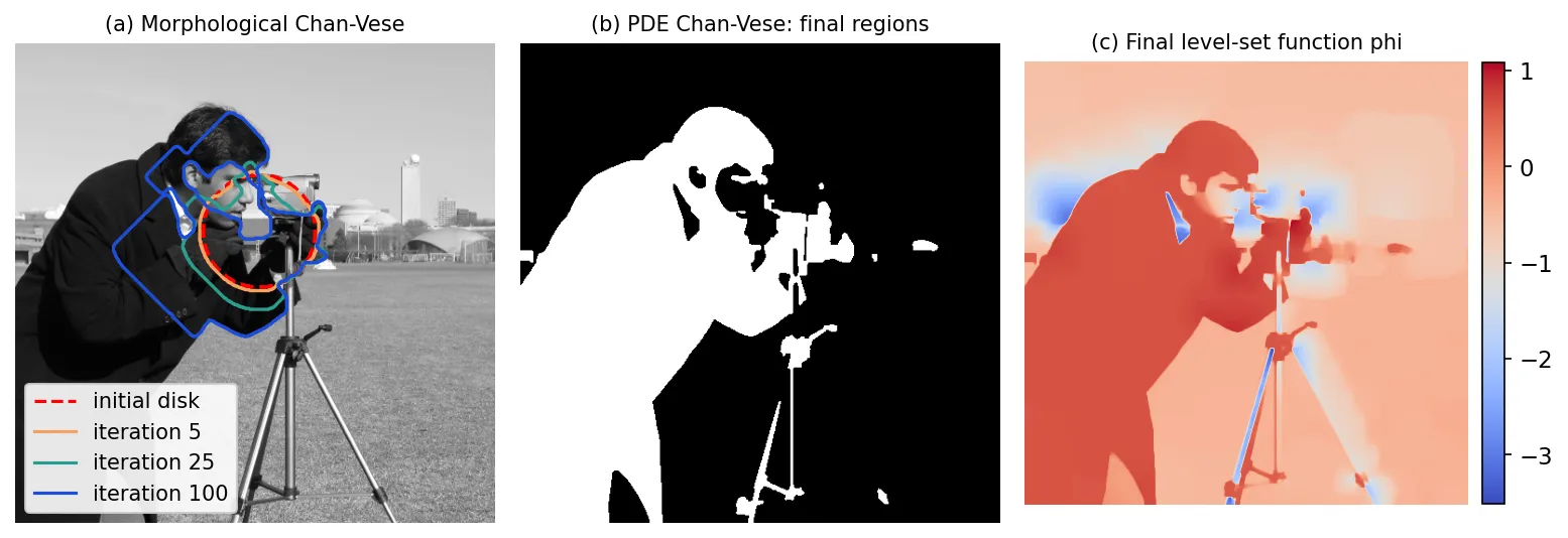

Initializing and reinitializing as a signed distance function

The initial $\phi$ is usually the signed distance to a user-drawn curve, a box, a disk, or many small circles (a “checkerboard”) so that the evolution starts near every possible object. As the PDE runs, $\phi$ drifts away from a distance function: it becomes very steep in some places and very flat in others. Steep regions force tiny time steps; flat regions make the zero crossing poorly located and sensitive to noise.

The classical remedy is reinitialization: every few iterations, replace $\phi$ by the signed distance to its current zero level set without moving that zero set. You can recompute it with a fast Euclidean distance transform, as in the code above, or solve a PDE that drives $\lvert\nabla\phi\rvert$ toward $1$ while freezing the sign of $\phi$. Reinitialization is effective but it can shift the front slightly, and deciding when to do it is a heuristic.

Li, Xu, Gui and Fox [10] proposed distance-regularized level-set evolution (DRLSE), which adds to the energy a penalty $\int p(\lvert\nabla\phi\rvert)$ whose minimum is at $\lvert\nabla\phi\rvert = 1$. The gradient flow of this penalty keeps $\phi$ close to a signed distance near the zero level set throughout the evolution, which removes the need for reinitialization.

Improving efficiency

A full-grid level-set solver updates every pixel at every step, although only the zero crossing matters. Three standard speed-ups:

• Narrow band. Adalsteinsson and Sethian [9] update $\phi$ only within a band of half-width $w$ (a few pixels) around the zero level set. When the front approaches the edge of the band, the band is rebuilt around the new front (with a reinitialization). The work per step drops from the image area to roughly the curve length times $w$.
• Larger stable steps. Semi-implicit or operator-splitting schemes allow larger $\Delta t$ for the stiff curvature term, at the cost of solving a linear system per step.
• Morphological approximations. Márquez-Neila, Baumela and Álvarez [11] replace the PDE by a sequence of binary morphological operators acting on a binary level set $u \in \{0, 1\}$. Dilation and erosion play the role of the balloon term, a composition of line-based sup-inf and inf-sup operators approximates curvature flow, and the sign of $\nabla g\cdot\nabla u$ implements the advection term. They prove that these operators have the same infinitesimal behavior as the PDE terms. The result is fast, has no time step, needs no reinitialization and never becomes unstable.

scikit-image provides morphological_geodesic_active_contour and morphological_chan_vese based on [11], alongside the PDE-based chan_vese [12]. Keep in mind that the morphological variants approximate the PDEs. They move on the pixel grid, their “smoothing” parameter is a number of operator applications rather than the weight $\mu$, and their results are close to, not identical with, the continuous models.

from skimage import data, img_as_float
from skimage.segmentation import (inverse_gaussian_gradient, disk_level_set,
                                  morphological_geodesic_active_contour)

coins = img_as_float(data.coins())
g = inverse_gaussian_gradient(coins, alpha=100, sigma=2)   # ~0 on edges, ~1 elsewhere
init = disk_level_set(coins.shape, radius=150)
mask = morphological_geodesic_active_contour(g, num_iter=250, init_level_set=init,
                                             smoothing=1, balloon=-1, threshold=0.69)

Here inverse_gaussian_gradient builds the edge-stopping function $g$, balloon=-1 shrinks the initial disk (the role of $c \lt 0$), and threshold decides which values of $g$ count as edges that stop the balloon.

Snakes vs level sets in practice

Both families minimize similar energies. The difference is mostly in representation, and the representation decides what is easy.

	Snakes (explicit)	Level sets (implicit)
Unknowns	$n$ points on the curve	one value per pixel (or per band pixel)
Cost per iteration	$O(n)$ after one matrix factorization	$O(\text{pixels})$, or $O(\text{band})$ with a narrow band
Topology changes	not without extra logic	automatic splitting and merging
Self-intersection	possible; must be detected	impossible by construction
Point spacing	drifts; needs resampling	no points to manage
Shape priors, landmarks, open curves	easy: points can carry labels	harder: no correspondence between iterations
Interactive editing	natural (drag a point)	indirect
Extension to 3D	meshes; harder bookkeeping	same equations on a voxel grid
Sub-pixel accuracy	yes	yes, by interpolating the zero crossing
Typical failure	stalls on clutter or in concavities	leaks through weak edges (edge-based); merges similar-looking regions (region-based)

Xu, Yezzi and Prince studied the relationship between the two formulations [3]; for many energies the choice is about implementation, not about what can be modeled in principle. A rule of thumb:

• Use a snake when you need one boundary of known topology, interactively, fast, or with point correspondences (tracking a contour across video frames, fitting a lip outline, delineating a building footprint).
• Use a level set when the number of objects is unknown, objects may touch or split, the boundary is ill-defined by gradients (region-based models), or you work in 3D.

Modern view

Active contours are no longer the default way to segment an image; deep networks are. But the ideas of this chapter, energies that combine boundary length with region fit, explicit contours deformed iteratively, and level sets as a shape representation, are still active ingredients in deep segmentation. Six papers give a good map.

Deformable models in medical imaging. McInerney and Terzopoulos [13] wrote the standard early survey of deformable models in medical image analysis. They frame snakes and their 3D relatives as energy-minimizing physical models and review applications to segmentation, shape representation, matching and motion tracking across CT, MRI and other modalities. Their main takeaway still holds: deformable models are most useful when the image alone is ambiguous and the model must contribute smoothness and prior knowledge.

Statistical region-based level sets. Cremers, Rousson and Deriche [14] review region-based level-set methods and derive them from a common Bayesian framework: each region gets a probability model (for intensity, color, texture or motion), and the level set maximizes the posterior probability of the partition, optionally with a statistical shape prior. Their argument for region-based energies, which are less sensitive to noise and have fewer local minima than edge-based snakes, is the reason Chan–Vese-type terms dominate later work.

A recent taxonomy of active contour models. Chen, Ge, Wang and Chen [15] sort active contour models into edge-based (GAC, DRLSE), region-based (Chan–Vese and local-fitting variants designed for intensity inhomogeneity) and hybrid models, implement a set of representative models, and compare them with deep learning segmentation on synthetic, medical and natural images. Their conclusion is pragmatic: classical models need no training data and give smooth closed boundaries, but they are sensitive to initialization and parameters; deep models are more accurate where labelled data exist; the two are complementary.

Shape constraints in deep segmentation. Bohlender, Oksuz and Mukhopadhyay [16] survey how anatomical shape knowledge is injected into deep medical image segmentation: conditional random fields, statistical shape models, active contours, and implicit shape representations such as signed distance maps. Their motivation is exactly the weakness active contours were designed to fix: pixel-wise classifiers can produce fragmented regions and topological errors.

Explicit contours learned end to end. Deep Snake by Peng et al. [17] keeps the snake’s representation, a closed polygon of vertices that is deformed iteratively, but replaces the energy-derived update with a learned one. Each vertex is described by CNN features sampled at its location, and a circular convolution along the polygon predicts per-vertex offsets toward the object boundary. Used for instance segmentation, it starts from a detector’s box, and the authors report real-time speed. The circular convolution plays the role that the pentadiagonal matrix $A$ played for the classical snake: it couples each vertex to its neighbours along the closed curve.

Active-contour energies as loss functions. Instead of running a contour at test time, several methods put the energy into the training loss:

• Chen et al. [18] propose a loss for medical image segmentation that adds a boundary-length term and inside/outside region-fitting terms, a supervised analogue of the Chan–Vese energy, to a dense segmentation network, and report improvements over cross-entropy on cardiac MRI.
• Kim and Ye [19] treat the softmax outputs of a network as the characteristic functions of regions and use a Mumford–Shah-style piecewise-constant energy as the loss. Because the energy needs no labels, the same loss supports unsupervised and semi-supervised segmentation, and it can act as a regularizer in supervised training.
• Kervadec et al. [20] propose the boundary loss, inspired by graph-based optimization of active-contour flows. It writes a distance between the predicted and true boundaries as a regional integral weighted by the signed distance map of the ground truth, which is exactly the level-set function of the true contour. It is designed for highly unbalanced problems, such as small lesions, where overlap losses alone train poorly, and is used together with a regional loss.

What deep learning changed, and what it did not:

• Changed: the data term. Hand-made forces ($\nabla e$, GVF, $g$, region means) are replaced by learned features. This is the main reason accuracy improved.
• Not changed: the regularity prior. Boundary length, curvature penalties, signed distance representations and region homogeneity reappear as loss terms and output representations, because pixel classifiers still produce ragged, fragmented boundaries without them.
• Not changed: the explicit vs implicit trade-off. Contour-based networks inherit the snake’s fixed topology (one polygon per instance) and its speed; mask and distance-map networks inherit the level set’s flexibility.
• Still useful on its own. When there are no labelled data, a Chan–Vese or GAC run is a few lines of scikit-image and needs no training, which makes it a good baseline, a pseudo-label generator, or a post-processing step that cleans up a network’s mask.

Key takeaways

• An active contour segments by minimizing an energy over curves: a regularity term (length, bending) plus a data term (edges or region fit). Gradient descent on that energy is a PDE in artificial time.
• A snake is an explicit chain of points. Its Euler–Lagrange equation $\alpha v_{ss} - \beta v_{ssss} + F_{\text{ext}} = 0$ is solved with a semi-implicit step $\mathbf{x}^t = (A + \gamma I)^{-1}(\gamma\mathbf{x}^{t-1} + \mathbf{f}_x)$.
• Plain gradient forces have a small capture range and fail in concavities. GVF diffuses edge vectors across the image; the balloon force inflates or deflates the curve.
• A level set stores the curve as $\{\phi = 0\}$ and evolves $\phi_t + F\lvert\nabla\phi\rvert = 0$ with upwind differences under a CFL step limit. Topology changes are automatic.
• The speed $F$ carries the model: geodesic active contours minimize edge-weighted length; Chan–Vese fits two region means and works without edges.
• Keep $\phi$ close to a signed distance (reinitialization or DRLSE), and save work with narrow bands or morphological approximations, which approximate rather than solve the PDEs.
• In deep learning the same ideas survive as learned contour deformation (Deep Snake) and as loss functions built from length, region and signed-distance terms.

Exercises

1. Tension alone. A closed snake with $\beta = 0$ and no external force is initialized as a circle of radius $R$ sampled at $n$ evenly spaced points. Using the discrete internal force $\alpha(v_{i+1} - 2v_i + v_{i-1})$, show that the circle stays a circle and find how its radius changes in one explicit step of size $\tau$.

Hint

For a regular polygon with angle step $\theta = 2\pi/n$, $v_{i+1} + v_{i-1} = 2\cos\theta\, v_i$ (measured from the centre). The force is $-2\alpha(1 - \cos\theta)\, v_i$, pointing to the centre, so $R \mapsto R\,[1 - 2\alpha\tau(1 - \cos\theta)]$. The circle shrinks geometrically; note that the rate depends on $n$, which is one reason snake parameters are tied to the sampling.

2. Concavity test. Using the gvf function above, build the U shape of Figure 11.2 and vary the GVF weight $\mu$ (0.05, 0.1, 0.2) and the number of GVF iterations. Which parameter controls how far the field reaches from the edges, and which controls how smooth it is?

Hint

The number of iterations sets how far diffusion can travel (roughly the square root of iterations times $\mu$). A larger $\mu$ also smooths more strongly, which helps against noise but rounds off small features. Above $\mu = 0.25$ the explicit scheme becomes unstable.

3. Signs and directions. With our convention ($\phi \lt 0$ inside), what happens to a circle under $\phi_t + F\lvert\nabla\phi\rvert = 0$ when $F = -1$? When $F = -\kappa$? Write the radius $r(t)$ in each case.

Answer

$F = -1$: the circle shrinks at unit speed, $r(t) = r_0 - t$. $F = -\kappa = -1/r$: curve-shortening flow, $\dot r = -1/r$, so $r(t) = \sqrt{r_0^2 - 2t}$, and the circle vanishes at $t = r_0^2/2$.

4. CFL in practice. Run the evolve snippet with cfl=0.5, 1.0 and 2.0 on the same circle. Measure the final radius and look at the zero contour. What breaks, and why does the narrow band not remove this limit?

Hint

Above 1 the front tries to cross more than one cell per step; upwind information comes from the wrong place and the contour becomes jagged or the values blow up. The narrow band reduces the number of pixels updated, not the size of each step.

5. When Chan–Vese fails. Create a synthetic image whose left half is a smooth gradient from black to white and whose right half contains a gray disc on a gray background of the same mean but different variance (add strong noise only inside the disc). Run chan_vese. Explain the result from the energy, and propose a change of the region model that would succeed.

Hint

Chan–Vese only compares means, so the disc (same mean) is invisible and the ramp is cut in the middle. Modeling each region by a Gaussian with its own mean and variance, as in the statistical framework of [14], makes the disc separable.

6. Energy as a loss. Write the Chan–Vese energy for a soft mask $m(x, y) \in [0, 1]$ (inside probability) instead of a level set, with the length term replaced by the total variation $\int \lvert\nabla m\rvert$. Show that for fixed $m$ the optimal $c_1, c_2$ are weighted means, and explain why this function can be used to train a network without labels.

Hint

$E = \mu\int\lvert\nabla m\rvert + \lambda_1\int m\,(f - c_1)^2 + \lambda_2\int (1 - m)(f - c_2)^2$. Setting $\partial E/\partial c_1 = 0$ gives $c_1 = \int m f / \int m$. Nothing in $E$ refers to ground truth, only to the image itself, so gradients with respect to the network producing $m$ exist without labels; compare with [19].

References

1. R. C. Gonzalez and R. E. Woods, Digital Image Processing, 4th ed., Pearson, 2018, Ch. 11. publisher page
2. M. Kass, A. Witkin, and D. Terzopoulos, “Snakes: Active contour models,” International Journal of Computer Vision, vol. 1, no. 4, pp. 321–331, 1988. doi:10.1007/BF00133570
3. C. Xu and J. L. Prince, “Snakes, shapes, and gradient vector flow,” IEEE Transactions on Image Processing, vol. 7, no. 3, pp. 359–369, 1998; see also C. Xu, A. Yezzi Jr., and J. L. Prince, “On the relationship between parametric and geometric active contours,” Proc. 34th Asilomar Conf. on Signals, Systems, and Computers, 2000. GVF project page with both papers
4. L. D. Cohen, “On active contour models and balloons,” CVGIP: Image Understanding, vol. 53, no. 2, pp. 211–218, 1991. author PDF
5. S. Osher and J. A. Sethian, “Fronts propagating with curvature-dependent speed: Algorithms based on Hamilton–Jacobi formulations,” Journal of Computational Physics, vol. 79, pp. 12–49, 1988. doi:10.1016/0021-9991(88)90002-2
6. V. Caselles, R. Kimmel, and G. Sapiro, “Geodesic active contours,” International Journal of Computer Vision, vol. 22, no. 1, pp. 61–79, 1997. PDF
7. D. Mumford and J. Shah, “Optimal approximations by piecewise smooth functions and associated variational problems,” Communications on Pure and Applied Mathematics, vol. 42, no. 5, pp. 577–685, 1989. doi:10.1002/cpa.3160420503
8. T. F. Chan and L. A. Vese, “Active contours without edges,” IEEE Transactions on Image Processing, vol. 10, no. 2, pp. 266–277, 2001. doi:10.1109/83.902291
9. D. Adalsteinsson and J. A. Sethian, “A fast level set method for propagating interfaces,” Journal of Computational Physics, vol. 118, pp. 269–277, 1995. summary page
10. C. Li, C. Xu, C. Gui, and M. D. Fox, “Distance regularized level set evolution and its application to image segmentation,” IEEE Transactions on Image Processing, vol. 19, no. 12, pp. 3243–3254, 2010. doi:10.1109/TIP.2010.2069690
11. P. Márquez-Neila, L. Baumela, and L. Álvarez, “A morphological approach to curvature-based evolution of curves and surfaces,” IEEE Transactions on Pattern Analysis and Machine Intelligence, 2014. doi:10.1109/TPAMI.2013.106
12. scikit-image developers, “skimage.segmentation” API reference (active_contour, chan_vese, morphological_chan_vese, morphological_geodesic_active_contour). docs
13. T. McInerney and D. Terzopoulos, “Deformable models in medical image analysis: A survey,” Medical Image Analysis, vol. 1, no. 2, 1996. author PDF
14. D. Cremers, M. Rousson, and R. Deriche, “A review of statistical approaches to level set segmentation: Integrating color, texture, motion and shape,” International Journal of Computer Vision, vol. 72, no. 2, pp. 195–215, 2007. doi:10.1007/s11263-006-8711-1
15. Y. Chen, P. Ge, G. Wang, and H. Chen, “An overview of intelligent image segmentation using active contour models,” Intelligence & Robotics, vol. 3, no. 1, pp. 23–55, 2023. open access
16. S. Bohlender, I. Oksuz, and A. Mukhopadhyay, “A survey on shape-constraint deep learning for medical image segmentation,” IEEE Reviews in Biomedical Engineering, vol. 16, pp. 225–240, 2023. arXiv:2101.07721
17. S. Peng, W. Jiang, H. Pi, X. Li, H. Bao, and X. Zhou, “Deep snake for real-time instance segmentation,” CVPR, 2020. arXiv:2001.01629
18. X. Chen, B. M. Williams, S. R. Vallabhaneni, G. Czanner, R. Williams, and Y. Zheng, “Learning active contour models for medical image segmentation,” CVPR, 2019. CVF open access
19. B. Kim and J. C. Ye, “Mumford–Shah loss functional for image segmentation with deep learning,” IEEE Transactions on Image Processing, vol. 29, pp. 1856–1866, 2020. doi · arXiv:1904.02872
20. H. Kervadec, J. Bouchtiba, C. Desrosiers, E. Granger, J. Dolz, and I. Ben Ayed, “Boundary loss for highly unbalanced segmentation,” Medical Image Analysis, vol. 67, 2021 (first presented at MIDL 2019). arXiv:1812.07032