Chapter 1 · Introduction

What you’ll learn

• What a digital image is, in words and as a function $f(x, y)$, and what “processing” one means
• Where image processing stops and computer vision begins, using the low-, mid- and high-level view
• How the field started: newspaper photos sent by telegraph, lunar probes, and medical scanners
• Which parts of the electromagnetic spectrum (and which non-light signals) produce the images we process
• The fundamental steps of image processing, which double as the roadmap for the 13 chapters of this series
• The hardware and software components of a working image processing system, and how deep learning is reshaping the camera pipeline

The big picture

Almost every image you look at today has passed through image processing before it reached your eyes. Your phone ran dozens of operations between the moment light hit its sensor and the moment the photo appeared on screen. A hospital CT scanner never takes a “photo” at all: it measures how X-rays are absorbed along thousands of lines and computes the picture. A weather satellite records energy the human eye cannot see and turns it into a map you can read.

This chapter is the map before the journey. It defines the field, tells you where it came from, shows the range of signals it handles, and lays out the steps that the remaining chapters cover one by one [1]. Nothing here is hard, but every later chapter refers back to the vocabulary we build now.

What is digital image processing?

Plain version. A picture becomes digital when we chop it into a grid of tiny squares and store one number (or a few numbers, for color) per square. Processing means feeding that grid of numbers to a computer and getting something useful back.

Images as functions

Mathematically, a grayscale image is a two-dimensional function

$$f(x, y), \qquad (x, y) \in \mathbb{R}^2 .$$

Here $x$ and $y$ are spatial coordinates, and the value $f(x, y)$ is the intensity (or gray level) of the image at that point. For a camera, intensity is proportional to the light energy that reached the sensor; for an X-ray film, to the radiation that passed through the body. In the real world $x$, $y$ and $f$ can all vary continuously.

An image is digital when all three quantities are finite and discrete. We sample the plane on an $M \times N$ grid and quantize each value to one of $L$ levels:

$$f : \{0, 1, \dots, M-1\} \times \{0, 1, \dots, N-1\} \to \{0, 1, \dots, L-1\}, \qquad L = 2^k .$$

$M$ is the number of rows, $N$ the number of columns, and $k$ the number of bits per value ($k = 8$ gives the familiar range 0 to 255). Each grid element is a pixel (short for picture element). Chapter 2 covers how sampling and quantization are chosen; for now it is enough to know that an image is a matrix.

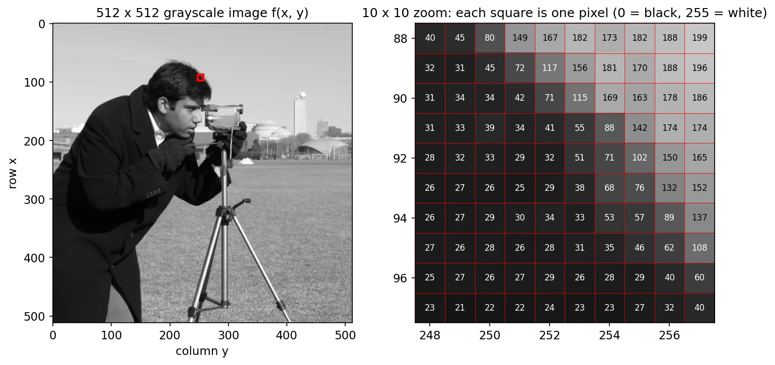
In code, this matrix is a NumPy array. Indexing with [row, column] reads a single pixel, and slicing returns a neighborhood:

from skimage import data

f = data.camera()            # a 512 x 512 grayscale photograph
print(f.shape, f.dtype)      # (512, 512) uint8
print(f[100, 250])           # intensity at row 100, column 250
print(f.min(), f.max())      # darkest and brightest values
patch = f[88:92, 248:252]    # a 4 x 4 neighborhood is just a sub-array
print(patch)

Color images add a third index for the channel, $f(x, y, c)$, and medical volumes add a depth index, $f(x, y, z)$. The ideas in this chapter carry over unchanged.

Where processing ends and vision begins

People disagree about where image processing stops and image analysis or computer vision starts. One extreme says image processing covers only operations whose input and output are both images. That rule is clean but too narrow: it would exclude something as simple as computing the average brightness of a photo. The other extreme is computer vision, whose goal is to emulate human vision: to understand a scene, recognize objects and act on them. Textbooks on vision treat it as a field in its own right, with geometry, 3-D reconstruction and recognition at its core [7].

A more useful picture is a continuum with three kinds of processes [1]:

• Low-level processes take an image in and give an image out. Examples: removing noise, increasing contrast, sharpening. No interpretation is involved.
• Mid-level processes take an image in and give attributes out: regions, edges, contours, or measurements of individual objects. Segmentation (splitting an image into meaningful parts) and describing those parts in a form a computer can sort are typical mid-level tasks.
• High-level processes “make sense” of a collection of recognized objects. Reading a whole page of text, or deciding that a medical scan shows a tumor, are high-level tasks. This end of the continuum is where image analysis merges into computer vision.

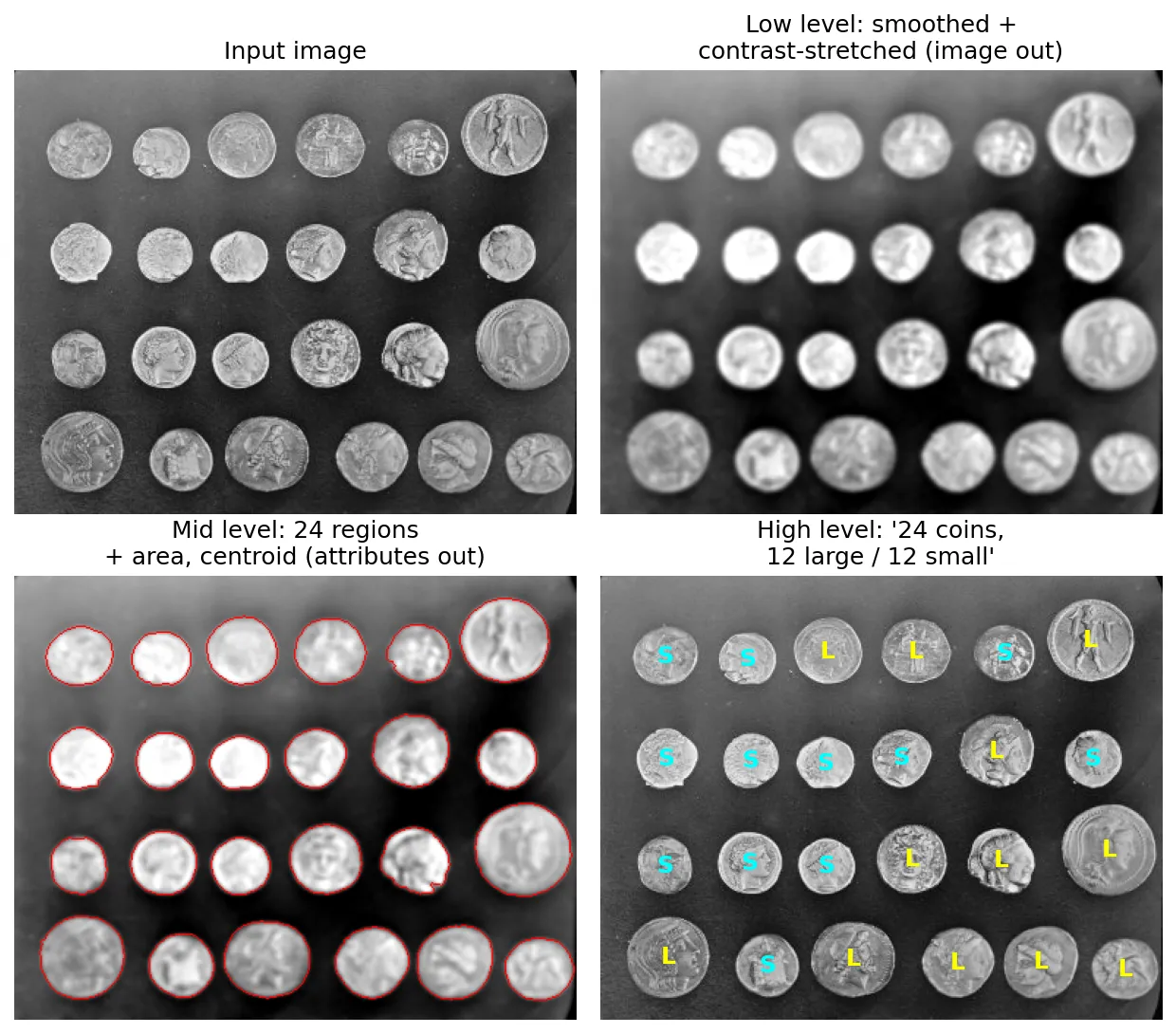
In this series, “digital image processing” means everything from the low level up to and including the recognition of individual regions or objects. That is wide enough to include segmentation, feature extraction and classification (Chapters 10–13), but it stops short of full scene understanding.

The origins of digital image processing

Plain version. The first digital pictures were newspaper photos sent across the Atlantic as punched telegraph tape. Real computer processing of images began in the 1960s, when space agencies needed to clean up pictures from lunar probes, and it exploded in the 1970s with medical scanners that build pictures from measurements.

Pictures over a telegraph cable

In the early 1920s, the Bartlane cable picture transmission system sent newspaper photographs between London and New York over the transatlantic submarine telegraph cable [2]. A photograph was converted into codes punched on ordinary five-unit telegraph tape, sent with standard telegraph equipment, and reassembled offline at the receiving end. According to Kobayashi’s history of the system, it carried nearly 500 news pictures across the Atlantic until the outbreak of war in 1939 [2]. The earliest Bartlane pictures used only five distinct gray levels; by the end of the 1920s the number had grown to fifteen [1].

Strictly speaking, no computer touched these pictures, so this is the prehistory of digital image processing. But the core idea was already there: a picture is turned into a finite set of codes, transmitted, and rebuilt, and the number of gray levels determines how faithful the result is.

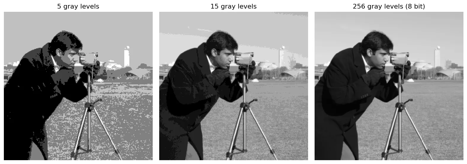
You can reproduce this experiment in a few lines. Uniform quantization to $L$ levels maps an intensity $r \in [0, 1]$ to

$$Q_L(r) = \frac{\operatorname{round}\big(r\,(L-1)\big)}{L-1},$$

where $\operatorname{round}$ rounds to the nearest integer, so the output takes only the $L$ values $0, \tfrac{1}{L-1}, \dots, 1$.

import numpy as np
from skimage import data

def quantize(img, levels):
    """Map a uint8 image onto `levels` evenly spaced gray levels."""
    x = img.astype(np.float64) / 255.0
    q = np.round(x * (levels - 1)) / (levels - 1)
    return (q * 255).astype(np.uint8)

f = data.camera()
for L in (5, 15, 256):
    g = quantize(f, L)
    print(L, "levels ->", len(np.unique(g)), "distinct values,",
          f"mean abs error {np.abs(g.astype(int) - f).mean():.2f}")

On the test image, the mean absolute error falls from about 18 gray levels with $L = 5$ to about 5 with $L = 15$, and to 0 with $L = 256$.

Computers meet images: the space program

Digital image processing as we know it needed two things that arrived only in the 1960s: computers powerful enough to hold and manipulate an image, and a problem important enough to pay for them. The space program provided both.

On 31 July 1964, the U.S. probe Ranger 7 took the first image of the Moon by a U.S. spacecraft, about 17 minutes before it crashed into the lunar surface as planned [3]. During those final minutes it returned more than 4,300 images, the last ones resolving details of about half a meter per pixel [3]. Using a computer to correct the distortions in such probe images became one of the founding projects of digital image processing [1]. The same techniques were then refined for later lunar and planetary missions.

Images computed from measurements: CT

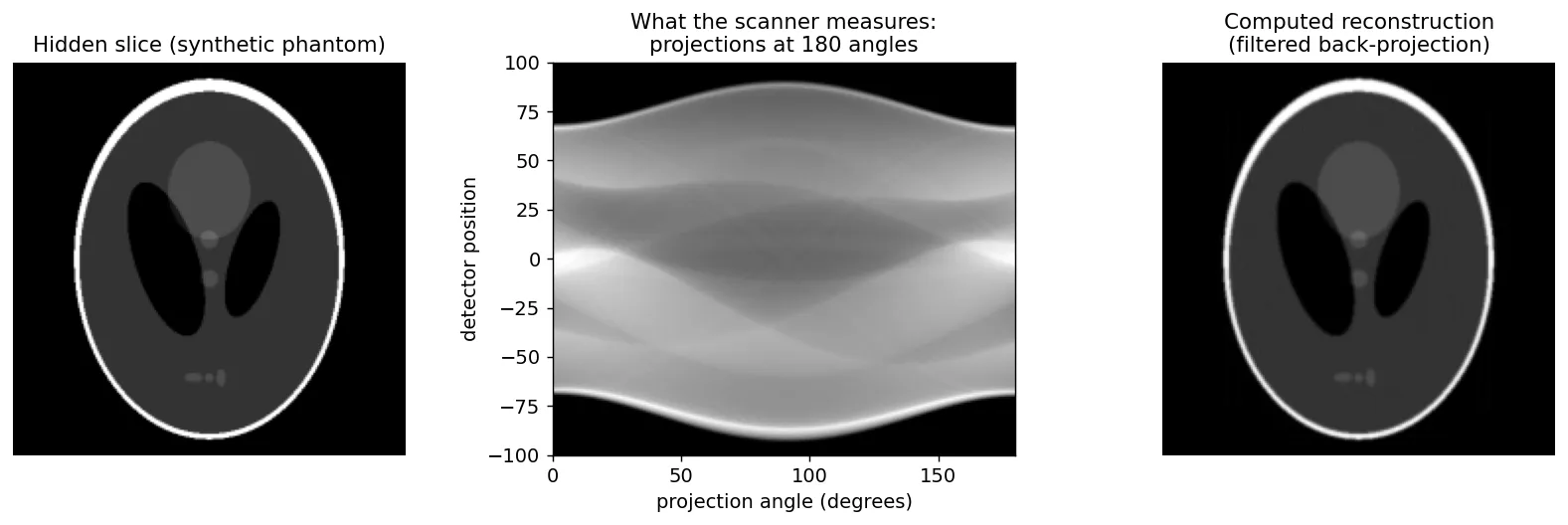
The second founding application came from medicine. In 1973, Godfrey Hounsfield described a system for computerized transverse axial scanning, now called computed tomography (CT) [4]. Instead of exposing one film, an X-ray source and detectors rotate around the patient and record how strongly the beam is absorbed along many lines at many angles. A computer then calculates the absorption at every point of a cross-section. Hounsfield reported that this revealed soft-tissue differences that conventional X-ray films could not show [4].

CT is a milestone because the image is not captured; it is reconstructed. The scanner measures line integrals of the unknown slice $f(x, y)$:

$$p(s, \theta) = \iint_{\mathbb{R}^2} f(x, y)\, \delta(x \cos\theta + y \sin\theta - s)\, dx\, dy ,$$

where $\theta$ is the angle of the beam, $s$ is the detector position along the projection, and $\delta$ is the Dirac delta, which keeps only the points on the line $x\cos\theta + y\sin\theta = s$. The collection of all projections $p(s, \theta)$ is the sinogram. Recovering $f$ from $p$ is an inverse problem, the subject of the reconstruction half of Chapter 5. The standard test object for such algorithms is a synthetic head slice made of ellipses, introduced by Shepp and Logan in 1974 [5].

import numpy as np
from skimage.data import shepp_logan_phantom
from skimage.transform import radon, iradon, rescale

slice_ = rescale(shepp_logan_phantom(), 0.5)           # 200 x 200 synthetic head slice
angles = np.linspace(0, 180, 180, endpoint=False)
sinogram = radon(slice_, theta=angles)                  # what the scanner records
recon = iradon(sinogram, theta=angles, filter_name="ramp")
err = np.sqrt(np.mean((recon - slice_) ** 2))
print(sinogram.shape, recon.shape, f"RMS error {err:.3f}")   # (200, 180) (200, 200) ~0.025

From the 1960s onward, the same ideas spread into remote sensing, astronomy, biology, industrial inspection, law enforcement and, eventually, every phone in every pocket. Two broad goals drive all of these applications: improving pictures for human interpretation, and processing image data for storage, transmission and machine perception.

Examples of fields that use digital image processing

Plain version. Our eyes see only a thin slice of the “light” that exists. Other kinds of light, from gamma rays to radio waves, can also make pictures, and so can sound and electron beams. Image processing works on all of them, because they all end up as grids of numbers.

The most useful way to organize applications is by the source of the image [1]. The main source is electromagnetic (EM) energy; others are acoustic waves, electrons, and pure computation.

The electromagnetic spectrum

EM waves can be described by wavelength $\lambda$ or frequency $\nu$, which are linked by

$$\lambda = \frac{c}{\nu},$$

where $c \approx 2.998 \times 10^8$ m/s is the speed of light. Light also comes in packets, photons, each carrying energy

$$E = h\nu = \frac{hc}{\lambda},$$

where $h \approx 6.626 \times 10^{-34}$ J·s is Planck’s constant. Short wavelength means high frequency and energetic photons; long wavelength means low frequency and gentle photons. That single fact explains much of imaging: energetic photons pass through tissue and metal (X-rays), while low-energy waves pass through clouds and darkness (radar and radio).

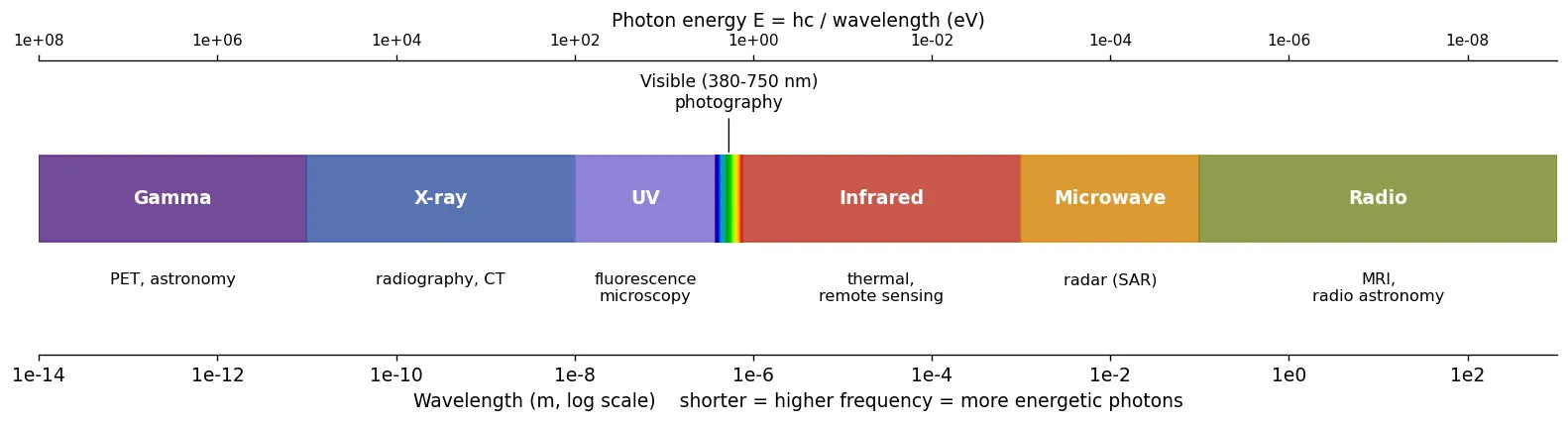
h, c, eV = 6.626e-34, 2.998e8, 1.602e-19   # Planck, speed of light, joules per eV

def photon_energy_ev(wavelength_m):
    return h * c / wavelength_m / eV

for name, lam in [("X-ray (0.1 nm)", 1e-10), ("green light (550 nm)", 550e-9),
                  ("thermal IR (10 um)", 10e-6), ("radar (3 cm)", 0.03)]:
    print(f"{name:22s} {photon_energy_ev(lam):10.3g} eV")
# X-ray ~1.24e4 eV, green ~2.25 eV, thermal IR ~0.124 eV, radar ~4.1e-5 eV

An X-ray photon carries roughly ten thousand times more energy than a photon of green light, and a radar photon carries less than a ten-thousandth of it. The bands below run from the most energetic to the least.

Gamma-ray imaging

Gamma rays are the most energetic photons. In nuclear medicine, a patient receives a radioactive tracer, and detectors record the gamma rays it emits; the image shows where the tracer collects, so it maps function (for example, metabolism) rather than anatomy. Positron emission tomography (PET) is a tomographic version of this idea and uses the same reconstruction mathematics as CT. In astronomy, gamma-ray telescopes image violent events such as the remains of exploded stars. Gamma-ray images are typically noisy, because every pixel counts a modest number of photon events; denoising and restoration (Chapters 3 and 5) matter here.

X-ray imaging

X-rays are the oldest medical imaging source. In a plain radiograph, X-rays pass through the body and expose a detector; dense tissue such as bone absorbs more and appears bright. Angiography injects a contrast agent into blood vessels and subtracts a pre-contrast image from a post-contrast one to isolate the vessels, which is an image arithmetic operation you will meet in Chapter 2. CT, described above, turns many X-ray projections into slices and stacks of slices [4]. Outside medicine, X-rays inspect welds and circuit boards for hidden defects, and X-ray telescopes image hot gas in galaxy clusters.

Ultraviolet imaging

Ultraviolet (UV) light sits just beyond violet. Its key application is fluorescence microscopy: some substances absorb UV photons and re-emit lower-energy visible light. Under a microscope that blocks the UV excitation and passes only the emitted light, the fluorescing structures glow against a dark background. Biologists tag specific proteins with fluorescent markers to see where they are in a cell. UV imaging is also used in astronomy and in industrial inspection, for example to reveal residues invisible in daylight.

Visible and infrared imaging

The visible band is where most everyday imaging happens: photography, light microscopy, industrial machine vision (checking that a pill packet is full, reading license plates, measuring parts), document scanning, and face and fingerprint analysis. The visible band is often combined with the nearby infrared (IR) band.

Remote sensing satellites record the same scene in several narrow bands from blue to infrared, called multispectral images. Because vegetation, water and soil reflect these bands differently, combining bands lets analysts map crops, floods or urban growth. Thermal infrared cameras sense emitted heat rather than reflected light, which makes them useful at night, in firefighting and in building inspection. Weather satellites use IR channels to track clouds and storms around the clock.

Microwave imaging (radar)

The dominant microwave imaging technology is imaging radar. A radar carries its own illumination: it sends microwave pulses and records the echoes. Because microwaves pass through clouds, haze and darkness, radar can image regions that optical satellites cannot see for weeks at a time, such as rainforests under constant cloud cover. Synthetic aperture radar (SAR) uses the motion of an aircraft or satellite to synthesize a very large antenna, giving fine resolution; turning the recorded echoes into an image is itself a computational step [8].

Radio-band imaging

At the long-wavelength end, the major application in medicine is magnetic resonance imaging (MRI). The patient lies in a strong magnetic field, short radio-frequency pulses excite hydrogen nuclei, and the faint radio signals they emit are recorded. In 1973, Paul Lauterbur showed that adding magnetic field gradients makes these signals depend on position, so an image can be formed from them [6]. Like CT, MRI produces an image only after computation: the raw measurements live in a frequency domain (the subject of Chapter 4) and must be transformed back.

In radio astronomy, the long wavelengths mean a single dish has poor resolution, so astronomers combine signals from many telescopes. In 2019, the Event Horizon Telescope Collaboration published the first image of the shadow of a supermassive black hole, at the center of the galaxy M87, made by combining data from radio observatories around the globe [9]. That image is as much the product of reconstruction algorithms as of the telescopes themselves.

Other imaging modalities

Not every image comes from EM radiation.

• Acoustic imaging. Sound waves reflect at boundaries between materials. Geologists send low-frequency sound into the ground and record echoes to map underground rock layers for oil, gas and mineral exploration (seismic imaging). Medical ultrasound uses high-frequency sound (millions of cycles per second) to image the fetus, the heart and abdominal organs in real time and without ionizing radiation. In both cases the image is formed by timing the echoes.
• Electron microscopy. Electrons can be focused like light, but their effective wavelength is far shorter, so electron microscopes resolve much finer detail than light microscopes. A transmission electron microscope passes a beam through a thin specimen; a scanning electron microscope sweeps a focused beam across a surface and records the electrons that bounce off or are knocked out. The images are often noisy and benefit from enhancement and restoration.
• Synthetic images. Computers also generate images that no sensor captured: fractals, rendered 3-D scenes, simulations, and, increasingly, images produced by generative models. These images are processed with the same tools, and they are widely used to create training data and test cases.

The lesson of this tour: once the data is a grid of numbers, the same toolbox applies, whether the numbers came from gamma rays, sound echoes or a computer program. What changes is the noise, the resolution and the physics of formation, and those differences decide which tool you reach for.

Fundamental steps in digital image processing

Plain version. Making an image useful is like cooking: you get the ingredients (acquire the image), clean and prepare them (enhance, restore), sometimes change their form (color, transforms, compression), then cut them into pieces (segmentation), describe each piece, and finally decide what each piece is (classification). You do not always need every step.

It helps to split the steps into two groups [1]: methods whose outputs are generally images, and methods whose outputs are generally attributes extracted from images. A knowledge base about the problem domain, such as where defects tend to appear or what a valid label looks like, guides every step. The list is not a mandatory pipeline; a given application uses only the steps it needs, in whatever order makes sense.

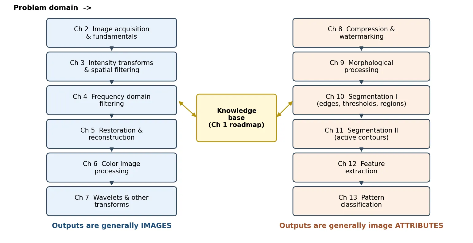
Here is each step, with the chapter that develops it.

1. Image acquisition — obtaining the image in digital form, including sensing, sampling and quantization. Chapter 2 also builds the mathematical toolkit (pixel relationships, arithmetic, geometric transforms) used everywhere else. → Chapter 2 · Digital Image Fundamentals
2. Image enhancement — making an image more suitable for a specific purpose, such as increasing contrast or sharpening detail. Enhancement is subjective: “better” depends on the viewer and the task. → Chapter 3 · Intensity Transformations and Spatial Filtering and Chapter 4 · Filtering in the Frequency Domain
3. Image restoration — undoing a known or estimated degradation such as blur or noise. Unlike enhancement, restoration is objective: it relies on mathematical models of how the image was degraded. The same chapter covers reconstruction from projections (CT). → Chapter 5 · Image Restoration and Reconstruction
4. Color image processing — color models, pseudo-color, and processing of full-color images. → Chapter 6 · Color Image Processing
5. Wavelets and other image transforms — representing images at several resolutions at once, the basis of modern compression and pyramid methods. → Chapter 7 · Wavelet and Other Image Transforms
6. Compression and watermarking — reducing the storage or bandwidth an image needs, and embedding invisible information to protect ownership. → Chapter 8 · Image Compression and Watermarking
7. Morphological processing — tools for extracting and cleaning up shape components, such as thinning, filling holes and separating touching objects. This is where outputs start to become attributes. → Chapter 9 · Morphological Image Processing
8. Segmentation — partitioning an image into its constituent parts or objects. It is one of the hardest steps, and errors here propagate to everything after it. → Chapter 10 · Image Segmentation I (edges, thresholds, regions) and Chapter 11 · Image Segmentation II (active contours: snakes and level sets)
9. Feature extraction — turning segmented regions into numbers: boundary and region descriptors, and point features such as corners. It has two parts: detecting features and describing them. → Chapter 12 · Feature Extraction
10. Image pattern classification — assigning a label to an object based on its features, from minimum-distance classifiers to neural networks and deep learning. → Chapter 13 · Image Pattern Classification

Chapter 1 (this page) is the overview that ties them together.

The following sketch strings four of these steps together on the coins image of Figure 1.2. Every step is one or two library calls here; the chapters explain what is going on inside each.

from scipy import ndimage as ndi
from skimage import data, filters, measure, segmentation

img = data.coins()

# 1) enhancement: low level, image in -> image out
smooth = filters.gaussian(img, sigma=1, preserve_range=True)

# 2) segmentation: mid level, image in -> regions out
markers = (smooth < 30) * 1 + (smooth > 150) * 2       # sure background / sure coin
regions = segmentation.watershed(filters.sobel(smooth), markers) == 2
regions = ndi.binary_fill_holes(regions)
labels = measure.label(regions)

# 3) feature extraction: regions in -> numbers out
props = [p for p in measure.regionprops(labels) if p.area > 300]
areas = [p.area for p in props]

# 4) classification / interpretation: numbers in -> a statement out
median = sorted(areas)[len(areas) // 2]
n_large = sum(a >= median for a in areas)
print(f"{len(areas)} coins found, {n_large} at or above the median size")
# 24 coins found, 12 at or above the median size

Notice the knowledge base hiding in this code: the thresholds 30 and 150, the minimum area 300 and the rule “large means at or above the median” all encode facts about this particular problem. Change the lighting or the coins and those numbers must change too. Much of the history of the field, including the rise of deep learning, is the story of moving such knowledge from hand-set constants into models learned from data.

Components of an image processing system

Plain version. An image processing system is a team: a sensor that catches the image, fast special-purpose chips that do the heavy lifting, a computer that runs the programs, memory that stores the pictures, a screen to look at them, a printer for paper copies, and a network that connects it all.

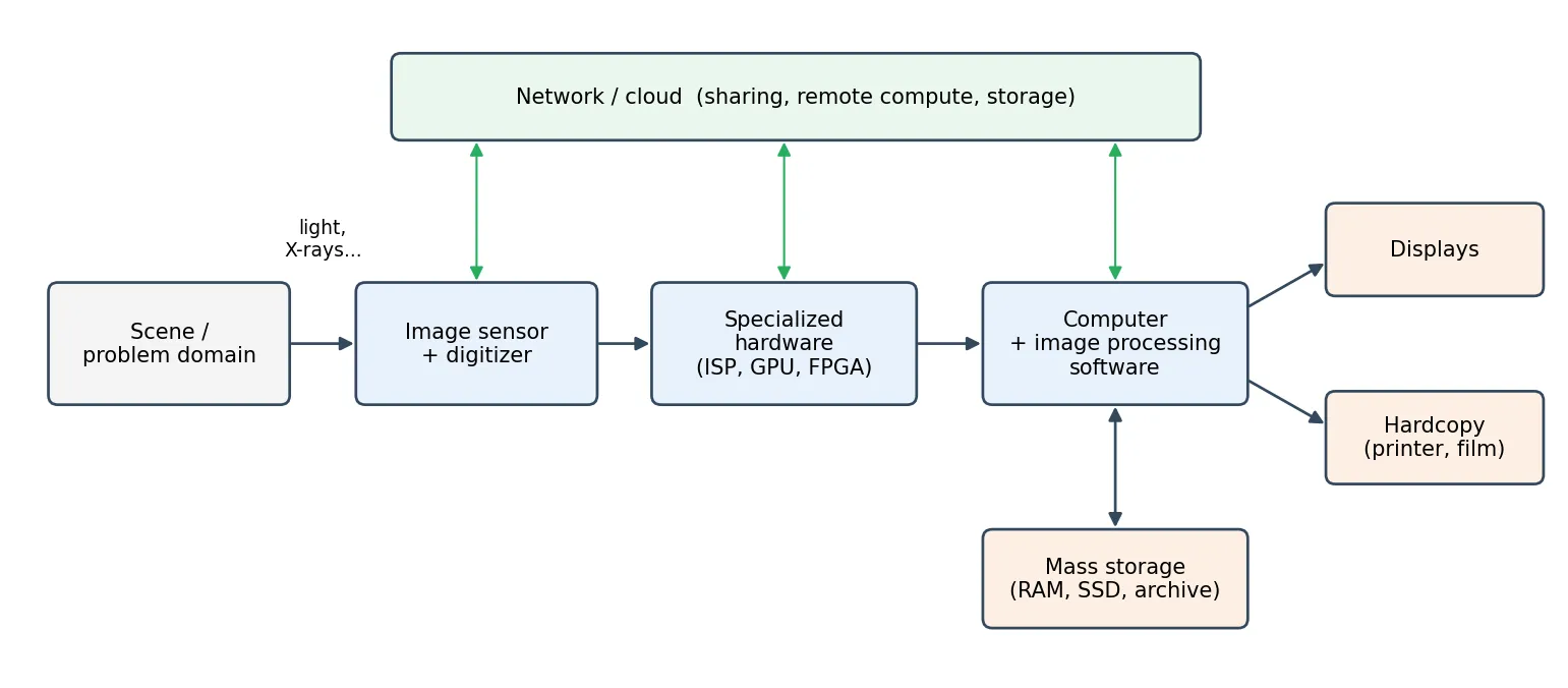
• Image sensors. Two elements are needed to acquire an image: a physical device that responds to the energy radiated by the object (a CCD or CMOS chip, an X-ray detector, an ultrasound transducer), and a digitizer that converts the device’s electrical output into numbers. In a phone, both sit on the same chip.
• Specialized image processing hardware. Some operations must run at video rate on every pixel, faster than a general-purpose processor can manage. Classic systems used dedicated arithmetic boards; today the role is filled by the image signal processor (ISP) inside every camera chip, by graphics processing units (GPUs), by field-programmable gate arrays (FPGAs), and by neural processing units in phones.
• The computer. Anything from an embedded microcontroller in a smart doorbell to a cluster of servers. For dedicated tasks, the computer may be customized; for research and general work, an ordinary workstation is enough.
• Software. Modules that perform specific tasks, plus a way to combine them. In this series we use Python with NumPy, SciPy, scikit-image and OpenCV. The ability to write your own code, rather than only call existing functions, is what this series aims to build.
• Mass storage. Images are large, and they arrive in bulk. Storage comes in three tiers: short-term storage during processing (RAM, GPU memory, frame buffers), online storage for fast recall (SSDs and disk arrays), and archival storage for rare access (tape, cold cloud storage).
• Image displays. Mostly color flat panels today. For medical diagnosis, specialized calibrated monitors are used, and for stereo or virtual reality, head-mounted displays.
• Hardcopy devices. Laser and inkjet printers, film cameras, and heat-sensitive printers. Film still offers very high resolution, and paper remains the medium of choice for written material and many reports.
• Networking and the cloud. Practically every system is now connected. Transmitting images is a bandwidth problem, which is why compression (Chapter 8) is a core topic. Cloud services move both storage and heavy computation (for example, training deep models) off the device.

How large is “large”? An image with $M$ rows, $N$ columns, $C$ channels and $k$ bits per value needs

$$b = M \times N \times C \times k \ \text{bits}$$

before compression, where $C = 1$ for grayscale and $C = 3$ for RGB color.

def raw_size_mb(height, width, channels=1, bits=8, frames=1):
    return height * width * channels * bits * frames / 8 / 1e6

print(f"{raw_size_mb(512, 512):.2f} MB   - this chapter's 8-bit test photo")         # 0.26
print(f"{raw_size_mb(3000, 4000, 3):.0f} MB   - one 12-megapixel RGB photo")         # 36
print(f"{raw_size_mb(512, 512, bits=16, frames=300):.0f} MB  - a 300-slice 16-bit CT volume")  # 157
print(f"{raw_size_mb(2160, 3840, 3, frames=30*60):.0f} MB - one minute of uncompressed 4K video")  # 44790

One minute of uncompressed 4K video at 30 frames per second is about 45 gigabytes. Without compression, streaming video and image-heavy web pages would be impractical.

Modern view

The textbook’s view of the field, a pipeline of well-understood, hand-designed steps, is still the right way to learn image processing. Two developments since about 2010 have changed how the field is practiced: computation has moved into the image formation itself, and learned models have replaced or augmented many hand-designed steps. The surveys below are good entry points.

Surveys on computational imaging and imaging beyond the visible

• Mait, Euliss and Athale, “Computational imaging” (2018) [8] review two decades of systems in which optics and computation are designed together, so that the sensor records data that is not a recognizable picture until it is processed. Their survey spans topics such as spatial light modulators, synthetic aperture radar and computational microscopy. The main takeaway is that the boundary between “acquisition” and “processing” in Figure 1.6 is now a design choice: CT, MRI and radar were early examples, and phones have made the approach mainstream.
• Delbracio, Kelly, Brown and Milanfar, “Mobile computational photography: a tour” (2021) [10] trace how phone cameras overcame their tiny sensors and lenses with algorithms: capturing a burst of frames and merging them, aggressive noise reduction, and multi-frame super-resolution. Their tour shows that a modern phone photo is the output of a long processing pipeline, and it is a useful companion to almost every chapter in this series.
• Gallego et al., “Event-based vision: a survey” (2020) [11] cover a sensor that breaks the frame-based model of Figure 1.1 entirely. An event camera pixel fires asynchronously whenever its own brightness changes, giving microsecond timing and very high dynamic range. The survey shows how classic tasks such as feature detection, optical flow and image reconstruction must be rethought when the input is a stream of events rather than a grid of numbers.
• Wang, Ye and De Man, “Deep learning for tomographic image reconstruction” (2020) [12] review how neural networks entered CT, MRI, PET and related modalities, the reconstruction problems that launched the field in the 1970s. They cover networks that clean up conventional reconstructions, physics-informed approaches that keep the measurement model in the loop, direct learned reconstruction, and generative models, with goals such as faster scans, lower radiation dose and better image quality. Their outlook stresses that large, well-curated datasets will be central to further progress.

How deep learning reshaped the processing pipeline

The broad shift is summarized in the review by LeCun, Bengio and Hinton (2015) [13]: deep networks learn representations of data at several levels of abstraction directly from examples, instead of relying on features designed by hand. For image processing, this has played out differently at each level of the continuum in Figure 1.2.

At the high level, the change has been nearly complete. Classification and recognition (Chapter 13) are now dominated by learned models; Chapters 12 and 13 explain the hand-designed features and classifiers that came before, which remain useful when data is scarce or interpretability matters.

At the low level, the clearest case study is the camera’s own processing pipeline. A conventional ISP is a chain of separately tuned stages that turn raw sensor values into a finished photo: black-level correction, demosaicing, denoising, white balance, color correction, tone mapping and compression. Ramanath et al. (2005) [14] give a clear overview of this pipeline and its trade-offs, and it is a good reference to keep next to Chapters 3, 5 and 6.

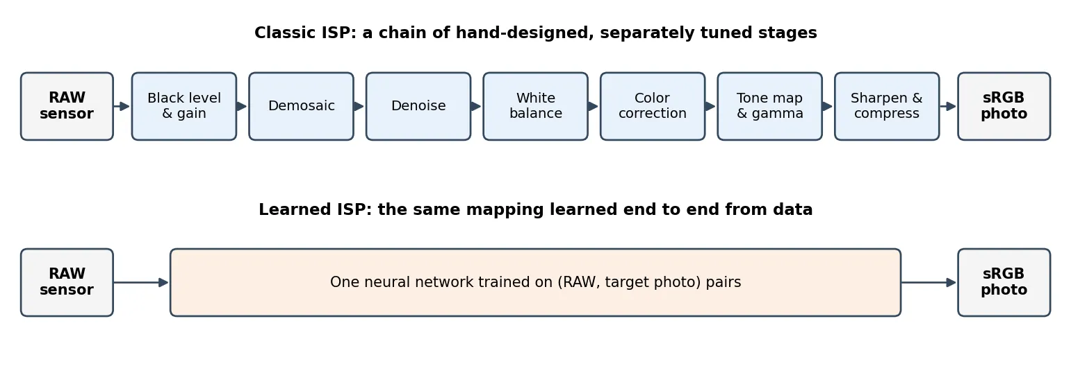
Deep learning has attacked this pipeline from several directions:

• Learning a hard stage end to end. Chen et al. (2018) trained a fully convolutional network to map short-exposure raw images taken in very low light directly to clean photos, using long-exposure shots of the same scenes as targets [15]. A traditional pipeline amplifies noise badly in this regime.
• Making training data realistic. Brooks et al. (2018) showed how to “unprocess” ordinary photos, inverting the steps of the camera pipeline to synthesize realistic raw data, so that denoising networks trained on it work on real sensor output [16]. This is a good example of classic pipeline knowledge making a learned model better.
• Replacing the whole ISP. Ignatov, Van Gool and Timofte (2020) proposed PyNET, a pyramid-shaped convolutional network that maps raw data from a smartphone sensor directly to a high-quality photo, learning demosaicing, denoising, color and tone in a single model [17]. They trained it on paired raw phone images and photos from a high-end DSLR camera of the same scenes.
• Surveying the space. da Silva et al. (2023) survey deep learning methods for image signal processing, comparing approaches that replace individual stages with those that replace the entire ISP with one network [18].

What did not change? The mathematics of image formation in Chapters 2, 4 and 5 still determines what any method, learned or not, can recover. Learned models are trained and evaluated with the quality measures, transforms and color spaces defined in the classic chapters. And many deployed systems are hybrids: a learned denoiser inside an otherwise conventional pipeline, or a physics-based reconstruction refined by a network [12]. Understanding the classic steps is what lets you see which part of such a system is doing what, and why it fails when it does.

Key takeaways

• A digital image is a function $f(x, y)$ sampled on an $M \times N$ grid and quantized to $L = 2^k$ levels; in code it is simply an array.
• Image processing spans a continuum: low-level (image to image), mid-level (image to attributes) and high-level (attributes to meaning). Computer vision lives at the high end.
• The field grew from telegraph picture transmission (1920s), computer correction of space-probe images (1960s) and computed medical images such as CT (1970s).
• Images come from every part of the EM spectrum, from gamma rays to radio waves, and from non-EM sources such as ultrasound, seismic waves and electron beams. The physics of the source determines noise and resolution, and so which tools you need.
• The fundamental steps split into steps whose outputs are images (acquisition through compression) and steps whose outputs are attributes (morphology through classification), all guided by domain knowledge. Chapters 2–13 follow this roadmap.
• A working system combines sensors, specialized hardware, a computer, software, storage, displays, hardcopy and networking.
• Deep learning has largely taken over high-level recognition and is reshaping low-level steps such as the camera ISP, but the classic models of image formation remain the foundation that learned methods build on.

Exercises

1. Storage budget. A microscope records a time-lapse of 16-bit grayscale images of size 2048 × 2048, one every 30 seconds for 48 hours. How much uncompressed storage does the experiment need? How many frames would fit on a 1 TB disk?

Hint

Each frame is $2048 \times 2048 \times 16$ bits $= 8{,}388{,}608$ bytes, about 8.4 MB. There are $48 \times 120 = 5760$ frames, so about 48 GB in total. A 1 TB disk holds roughly $10^{12} / 8.39 \times 10^{6} \approx 119{,}000$ frames.

2. Place it on the continuum. Classify each task as low-, mid- or high-level, and justify your answer: (a) removing salt-and-pepper noise from a scanned page; (b) outlining every cell in a microscope image and reporting each cell’s area; (c) deciding whether a chest X-ray is normal; (d) brightening a dark photo.

Hint

Ask what comes out. An image out means low level ((a), (d)). Regions or measurements out means mid level ((b)). A judgment about the scene means high level ((c)).

3. Why X-rays and not light? Using $E = hc/\lambda$, compute the photon energy of a 0.05 nm X-ray and of 600 nm orange light. Explain in two sentences why the first is used to image bones and the second is not.

Hint

About 24.8 keV versus about 2.07 eV, a ratio of roughly 12,000. Visible photons are absorbed or scattered within millimeters of tissue; high-energy X-ray photons pass through soft tissue, and bones absorb a larger share of them, which produces contrast.

4. How many gray levels? Using the quantize function from this chapter, plot the mean absolute error between data.camera() and its quantized version for $L = 2, 3, \dots, 32$. Then look at the images. Around which $L$ do false contours stop being obvious to you? Is the error curve a good predictor of what you see?

Hint

For uniform quantization the error falls roughly as $1/L$. Visible banding depends on the smooth areas of the image (here, the sky) more than on the average error, which is one reason Chapter 2 treats perceived quality separately from numerical error.

5. Design a system. A factory wants to reject cracked ceramic tiles moving on a conveyor belt at two tiles per second. List the components of Figure 1.7 you would need, and for each of the fundamental steps of Figure 1.6, say whether you would use it and why.

Hint

You need a sensor with controlled lighting, enough compute to process two images per second, and a link to the reject mechanism. Likely steps: acquisition, enhancement (contrast), perhaps morphology, segmentation of crack-like structures, features (crack length), and a classification rule. Color, wavelets and compression are probably unnecessary, unless images are archived for audit.

6. Learned or classic? Pick one stage of the classic ISP in Figure 1.8. Give one argument for replacing it with a learned model and one argument for keeping the hand-designed version.

Hint

For learning: a network can adapt to the actual sensor noise and scene statistics. For keeping it: a hand-designed stage is predictable, cheap to run, easy to tune and does not need paired training data. Several references in the Modern view discuss exactly this trade-off.

References

1. R. C. Gonzalez and R. E. Woods, Digital Image Processing, 4th ed., Pearson, 2018, Ch. 1. publisher page
2. K. Kobayashi, “Birth of a Digital Phototelegraph — the Bartlane System,” Journal of the Institute of Image Electronics Engineers of Japan, vol. 31, no. 2, pp. 244–249, 2002. J-STAGE
3. NASA, “First Image of the Moon Taken by a U.S. Spacecraft” (Ranger 7, PIA02975), NASA Photojournal. NASA
4. G. N. Hounsfield, “Computerized transverse axial scanning (tomography): Part 1. Description of system,” British Journal of Radiology, vol. 46, no. 552, pp. 1016–1022, 1973. doi:10.1259/0007-1285-46-552-1016
5. L. A. Shepp and B. F. Logan, “The Fourier reconstruction of a head section,” IEEE Transactions on Nuclear Science, vol. 21, no. 3, pp. 21–43, 1974. doi:10.1109/TNS.1974.6499235
6. P. C. Lauterbur, “Image formation by induced local interactions: examples employing nuclear magnetic resonance,” Nature, vol. 242, pp. 190–191, 1973. doi:10.1038/242190a0
7. R. Szeliski, Computer Vision: Algorithms and Applications, 2nd ed., Springer, 2022. book site
8. J. N. Mait, G. W. Euliss and R. A. Athale, “Computational imaging,” Advances in Optics and Photonics, vol. 10, no. 2, pp. 409–483, 2018. doi:10.1364/AOP.10.000409
9. The Event Horizon Telescope Collaboration, “First M87 Event Horizon Telescope Results. I. The Shadow of the Supermassive Black Hole,” The Astrophysical Journal Letters, vol. 875, no. 1, 2019. doi:10.3847/2041-8213/ab0ec7
10. M. Delbracio, D. Kelly, M. S. Brown and P. Milanfar, “Mobile Computational Photography: A Tour,” arXiv:2102.09000, 2021. arXiv
11. G. Gallego et al., “Event-based Vision: A Survey,” IEEE Transactions on Pattern Analysis and Machine Intelligence, 2020. arXiv
12. G. Wang, J. C. Ye and B. De Man, “Deep learning for tomographic image reconstruction,” Nature Machine Intelligence, vol. 2, no. 12, pp. 737–748, 2020. doi:10.1038/s42256-020-00273-z
13. Y. LeCun, Y. Bengio and G. Hinton, “Deep learning,” Nature, vol. 521, pp. 436–444, 2015. doi:10.1038/nature14539
14. R. Ramanath, W. E. Snyder, Y. Yoo and M. S. Drew, “Color image processing pipeline,” IEEE Signal Processing Magazine, vol. 22, no. 1, pp. 34–43, 2005. doi:10.1109/MSP.2005.1407713
15. C. Chen, Q. Chen, J. Xu and V. Koltun, “Learning to See in the Dark,” CVPR, 2018. arXiv
16. T. Brooks, B. Mildenhall, T. Xue, J. Chen, D. Sharlet and J. T. Barron, “Unprocessing Images for Learned Raw Denoising,” arXiv:1811.11127, 2018. arXiv
17. A. Ignatov, L. Van Gool and R. Timofte, “Replacing Mobile Camera ISP with a Single Deep Learning Model,” arXiv:2002.05509, 2020. arXiv
18. M. H. M. da Silva et al., “ISP meets Deep Learning: A Survey on Deep Learning Methods for Image Signal Processing,” arXiv:2305.11994, 2023. arXiv