Chapter 2 · Digital Image Fundamentals

What you’ll learn

• How the human eye senses light, and why what we see is not always what is there (brightness adaptation, the Weber ratio, Mach bands, simultaneous contrast)
• Where images come from physically: the electromagnetic spectrum, sensors, and the illumination–reflectance model $f = i \cdot r$
• What sampling and quantization do, how they set spatial and intensity resolution, and how nearest, bilinear and bicubic interpolation resize an image
• The vocabulary of pixel relationships: neighbors, adjacency, connectivity, regions, boundaries, and three distance measures
• The mathematical toolbox used in every later chapter: elementwise vs matrix operations, linearity, arithmetic, set and logical operations, geometric transforms, image transforms, and histograms as probabilities

The big picture

Chapter 1 told us what digital image processing is. This chapter explains what a digital image actually is, starting from the light that leaves a scene and ending with a grid of integers in memory. Along the way it defines the words — pixel, neighbor, resolution, linear operator — that the rest of the series uses without stopping to explain.

Two things make this chapter more than bookkeeping. First, the final consumer of most images is a human, so we need to know where the eye is easily fooled and where it is sharp. Second, every choice made when an image is captured — how many samples, how many levels, which interpolation — leaves a fingerprint that later algorithms must live with. Deep networks did not remove these choices; they mostly moved them into training data and loss functions, as the Modern view section shows.

Elements of visual perception

In plain words: your eye is a camera made of jelly and nerve cells. It is extremely good at seeing differences and edges, and surprisingly bad at judging absolute brightness.

Structure of the eye and image formation

Light enters through the cornea, passes the pupil (whose size the iris controls), and is focused by the lens onto the retina, a thin layer of light receptors at the back of the eye [1]. The lens is flexible: ciliary muscles change its curvature, which changes its focal length so that near and far objects can both be brought into focus. The retinal image is real and inverted, just like the image on a camera sensor.

The retina contains two kinds of receptor [1]:

• Cones — a few million per eye, packed most densely in a small central pit called the fovea. They work in bright light (photopic vision), come in three types with different spectral sensitivities, and give us color and fine detail. Many cones have their own nerve connection, which is why foveal vision is sharp.
• Rods — many times more numerous, spread across the retina, absent from the center of the fovea. They work in dim light (scotopic vision), have no color discrimination, and many rods share one nerve ending, trading detail for sensitivity. This is why objects seen by moonlight look colorless and soft.

The point where the optic nerve leaves the eye has no receptors at all: the blind spot. You do not notice it because the brain fills in the gap — an early hint that perception is an active reconstruction, not a recording.

Brightness adaptation and discrimination

The visual system copes with an enormous range of light levels, from starlight to sunlight. It does this by brightness adaptation: at any moment it operates over a much narrower window centered on the current adaptation level, and that window slides as the overall light changes [1]. Within the window, subjective brightness grows roughly with the logarithm of the physical light intensity, not linearly.

How small a change can we notice? Put a uniform field of intensity $I$ in front of an observer and flash a small spot of intensity $I + \Delta I$. The increment that is noticed half of the time is $\Delta I_c$. The ratio

$$W = \frac{\Delta I_c}{I}$$

is the Weber ratio, where $I$ is the background intensity and $\Delta I_c$ is the just-noticeable increment. A small $W$ means good discrimination (a small relative change is visible). Over a wide middle range of intensities $W$ is roughly constant, which is Weber’s law: what we perceive is the relative change, not the absolute one. At low intensities, where rods dominate, $W$ is large and discrimination is poor [1].

This has a direct engineering consequence. Because we perceive relative changes, equally spaced physical gray levels are not equally spaced perceptually. That is one reason images are stored with a nonlinear (gamma) encoding, and one reason 8 bits are usually enough for display.

Mach bands, simultaneous contrast and illusions

Perceived brightness is not a simple function of intensity. Two classic demonstrations make this obvious [1]:

• Mach bands. Show a staircase of flat gray stripes. Each stripe is physically uniform, yet observers report a thin darker band on the dark side of every edge and a thin brighter band on the bright side. The visual system exaggerates edges, a behavior consistent with lateral inhibition between neighboring receptive fields — essentially a built-in sharpening filter.
• Simultaneous contrast. A mid-gray square looks lighter on a dark background and darker on a light one, although the square is identical in both cases. Perceived brightness depends on the surround.

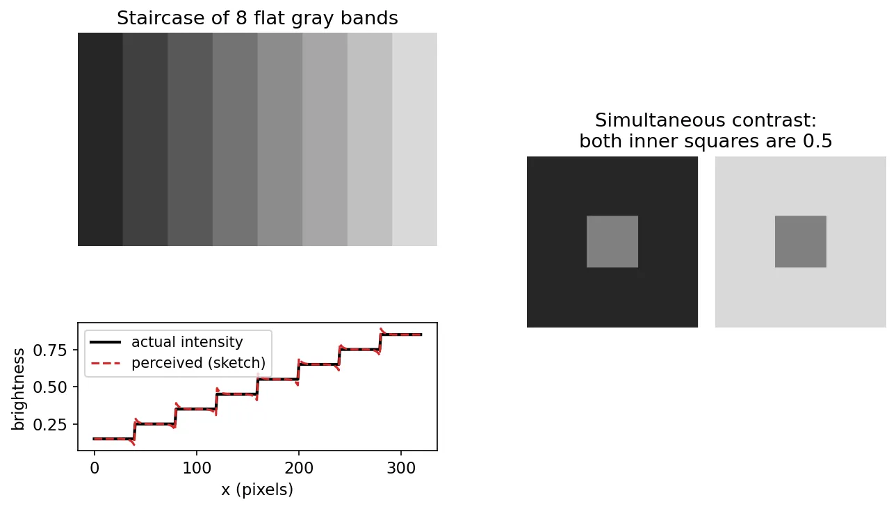
Optical illusions in general — contours that are not drawn, lines of equal length that look unequal — show that the eye fills in and reinterprets. For image processing this matters twice: an algorithm that minimizes squared error may still produce images that look wrong, and an artifact that is numerically small may be very visible if it sits on an edge. This is the starting point of perceptual quality metrics, discussed in the Modern view.

Light and the electromagnetic spectrum

In plain words: light is a wave of energy. Visible light is a thin slice of a much wider spectrum that also includes radio, microwaves, infrared, ultraviolet, X-rays and gamma rays — and images can be made from any of them.

Wavelength, frequency and energy

Electromagnetic radiation can be described as a sinusoidal wave or as a stream of massless particles called photons [1]. The two descriptions are linked by

$$\lambda = \frac{c}{\nu}, \qquad E = h\nu,$$

where $\lambda$ is the wavelength (meters), $\nu$ is the frequency (hertz), $c \approx 3 \times 10^{8}$ m/s is the speed of light, $E$ is the energy of one photon (joules), and $h$ is Planck’s constant. Shorter wavelength means higher frequency and higher energy per photon. That is why gamma rays and X-rays can pass through tissue, while radio waves need large antennas to be detected.

The visible band spans roughly 400 nm (violet) to 700 nm (red). An object’s perceived color is determined by which wavelengths it reflects: a green leaf reflects mostly in the middle of the band and absorbs the rest. Light with no color, only intensity, is called achromatic or monochromatic, and its intensity is called the gray level.

Radiance, luminance and brightness

Three words are easily confused [1]:

• Radiance — the total energy flowing from the light source, measured in watts. It is purely physical.
• Luminance — the amount of that energy an observer perceives, measured in lumens. It weights radiance by the eye’s spectral sensitivity: an infrared source can have high radiance but almost zero luminance.
• Brightness — the subjective sensation of intensity. It cannot be measured directly and, as the previous section showed, depends on adaptation and surroundings.

A sensor’s sensitivity curve plays the role of the eye’s: an image is only as good as the match between the band a sensor detects and the wavelength the object emits or reflects. To image an object, the wavelength must also be comparable to or smaller than the object’s size — one reason electron microscopes, with very short effective wavelengths, resolve far smaller structures than light microscopes.

Image sensing and acquisition

In plain words: a sensor is a tiny light meter that turns light into voltage. Put many of them in a row or a grid and you have a scanner or a camera.

Single, line and array sensors

Every imaging device combines an illumination source, the scene, and a sensor whose material responds to the energy of interest [1]. The sensor’s output voltage is digitized to give one number. Sensors are arranged in three ways:

• Single sensor. One detector (for example a photodiode) plus mechanical motion in two directions sweeps out an image one sample at a time. Slow, but cheap and very precise; used in some high-precision scanners.
• Line (strip) sensor. A row of detectors captures one line at a time, and motion perpendicular to the strip provides the second dimension. Flatbed scanners and airborne push-broom imagers work this way. A ring of sensors around a rotating source is the geometry of computed tomography (CT), where the image is reconstructed rather than read out directly.
• Array sensor. A 2-D grid of detectors, such as a CCD or CMOS chip, captures the whole image at once. This is the digital camera. A lens focuses the scene onto the array, each detector integrates light over an exposure time, and the readout electronics produce one value per detector.

Color cameras usually place a mosaic of red, green and blue filters over the array, so each detector measures only one color; the missing two values per pixel are interpolated (demosaicked) in the camera’s image-processing pipeline [8].

A simple image formation model

We write a monochrome image as a 2-D function $f(x, y)$ whose value is proportional to the energy arriving at $(x, y)$. Because it comes from physical energy, $0 \le f(x, y) \lt \infty$. For reflected light, it helps to split $f$ into two factors [1]:

$$f(x, y) = i(x, y)\, r(x, y), \qquad 0 \lt i(x, y) \lt \infty, \qquad 0 \lt r(x, y) \lt 1,$$

where $i(x, y)$ is the illumination (how much light falls on the scene point) and $r(x, y)$ is the reflectance (what fraction of it the surface reflects, from total absorption near 0 to total reflection near 1). Illumination depends on the light source; reflectance is a property of the object. For transmission imaging such as X-rays, a transmissivity takes the place of reflectance.

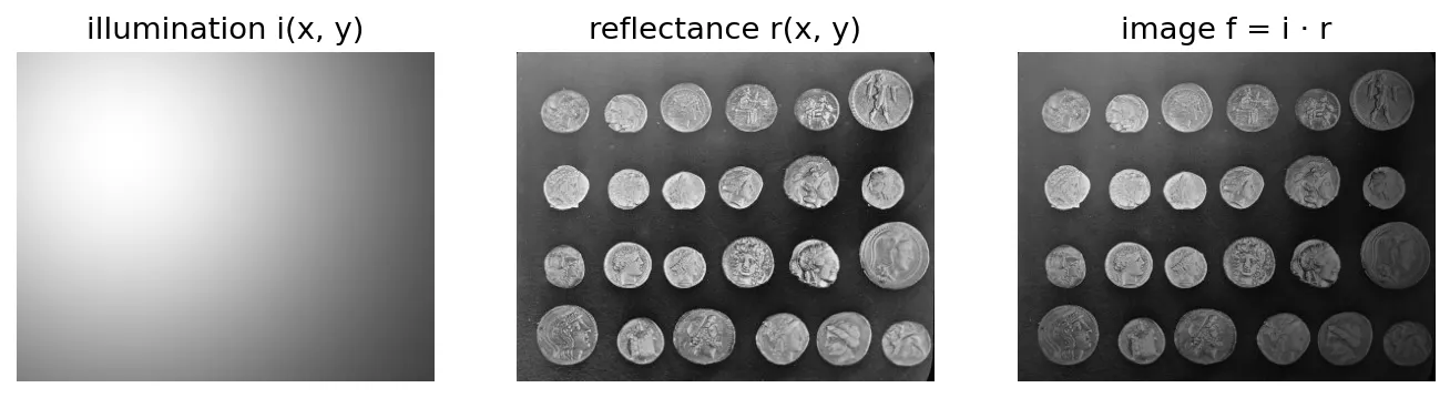
import numpy as np
from skimage import data, img_as_float

r = img_as_float(data.coins())          # reflectance in [0, 1]
h, w = r.shape
yy, xx = np.mgrid[0:h, 0:w]
i = 0.2 + 0.8 * xx / (w - 1)            # illumination ramp: dim left, bright right
f = i * r                               # what the sensor records

The model is simple but useful. Illumination usually varies slowly across a scene, while reflectance changes abruptly at object edges. Later chapters exploit this: homomorphic filtering (Chapter 4) takes $\log f = \log i + \log r$ to separate the two, and shading correction (later in this chapter) divides out a known $i$.

Image sampling and quantization

In plain words: a camera measures a continuous scene at a finite number of points (sampling) and rounds each measurement to one of a finite number of levels (quantization).

Basic concepts

A sensor’s output is a continuous voltage waveform over a continuous plane. To make it digital, both the coordinates and the amplitude must become discrete [1]:

• Sampling digitizes the coordinates: we keep values only at a grid of positions.
• Quantization digitizes the amplitude: each kept value is mapped to the nearest of a finite set of levels.

With an array sensor, the number and spacing of detectors fix the sampling; the analog-to-digital converter fixes the quantization. How finely we must sample depends on the image content: by the sampling theorem, a band-limited signal can be reconstructed exactly if it is sampled at more than twice its highest frequency. Chapter 4 develops this properly; Unser’s review gives the modern, spline-based view of sampling and reconstruction [2].

Representing digital images

After sampling and quantization, an image is a matrix of $M$ rows and $N$ columns:

$$f = \begin{bmatrix} f(0,0) & f(0,1) & \cdots & f(0,N-1) \\ f(1,0) & f(1,1) & \cdots & f(1,N-1) \\ \vdots & \vdots & \ddots & \vdots \\ f(M-1,0) & f(M-1,1) & \cdots & f(M-1,N-1) \end{bmatrix}$$

Each element is a pixel (picture element). Following the book’s convention [1], $x$ indexes rows and $y$ indexes columns, with the origin at the top-left corner. (Many libraries, including OpenCV’s point APIs, use $(x, y)$ = (column, row). Always check.)

The number of intensity levels is normally a power of two, $L = 2^k$, so values lie in $[0, L-1]$. Storing the image takes

$$b = M \times N \times k \ \text{bits},$$

where $k$ is the number of bits per pixel. A $512 \times 512$ image with $k = 8$ needs 262,144 bytes. The dynamic range of an imaging system is the ratio of the largest measurable intensity (set by saturation) to the smallest (set by noise); the contrast of a particular image is the difference between its highest and lowest intensities.

Spatial and intensity resolution

Spatial resolution is the size of the smallest discernible detail. It is meaningful only with units: line pairs per millimeter, or dots per inch (dpi) in printing. Saying an image is “1024 × 1024” says nothing about resolution until we know the physical area it covers. Intensity resolution is the smallest discernible change in level, usually stated as the number of bits $k$.

import numpy as np
from skimage import data

img = data.camera()                       # 512 x 512, uint8 (k = 8)
small = img[::4, ::4]                     # keep every 4th sample -> 128 x 128

def quantize(x, bits):
    step = 2 ** (8 - bits)
    return (x // step) * step + step // 2 # map to the centre of each bin

q3 = quantize(img, 3)                     # 8 gray levels
print(small.shape, np.unique(q3).size)    # (128, 128) 8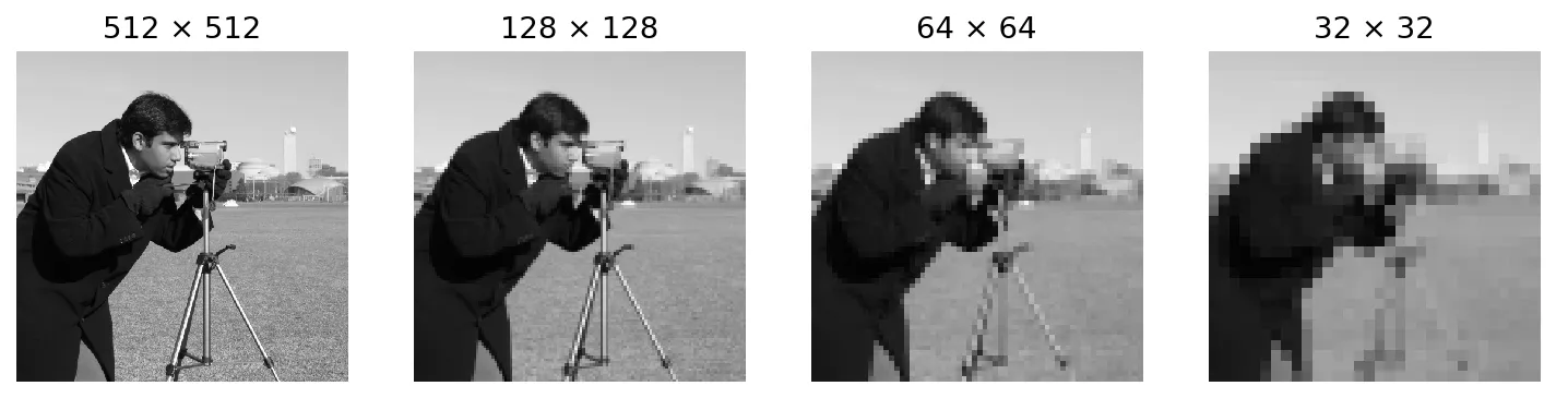

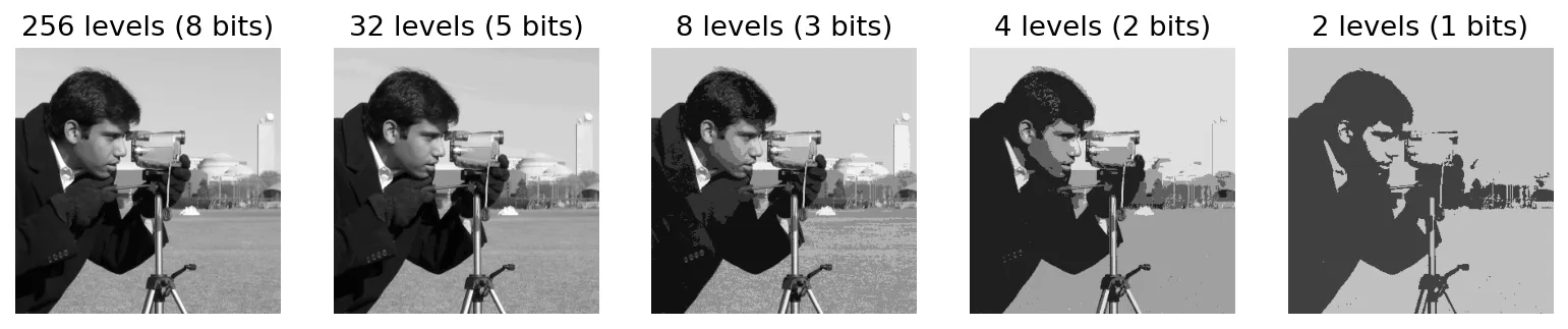
Two lessons follow. Reducing samples first destroys fine texture (grass, hair), then edges. Reducing levels first damages smooth regions: the sky in Figure 2.4 breaks into visible steps called false contouring, exactly where the Weber ratio says the eye is most sensitive. Images with a lot of detail tolerate fewer gray levels than smooth ones, because busy texture masks the steps [1].

Image interpolation

Interpolation estimates values at positions where we have no samples. It is used whenever an image is resized, rotated, warped or registered [1], [3], [4].

Nearest neighbor copies the value of the closest sample. It is fast and keeps the original values, but it makes edges blocky and, when shrinking, can drop thin structures entirely.

Bilinear interpolation uses the four nearest samples. For a point at fractional offsets $a, b \in [0, 1)$ from the top-left sample $f_{00}$,

$$v = (1-a)(1-b)\, f_{00} + a(1-b)\, f_{01} + (1-a)b\, f_{10} + ab\, f_{11},$$

where $f_{01}$, $f_{10}$ and $f_{11}$ are the right, lower and lower-right neighbors. Equivalently, $v(x, y) = c_1 x + c_2 y + c_3 xy + c_4$, with the four coefficients fixed by the four samples. The result is continuous but slightly blurred.

import numpy as np

def bilinear(img, x, y):
    """Sample img (H, W) at real-valued column x, row y."""
    x0, y0 = int(np.floor(x)), int(np.floor(y))
    x1, y1 = min(x0 + 1, img.shape[1] - 1), min(y0 + 1, img.shape[0] - 1)
    a, b = x - x0, y - y0
    top = (1 - a) * img[y0, x0] + a * img[y0, x1]
    bot = (1 - a) * img[y1, x0] + a * img[y1, x1]
    return (1 - b) * top + b * bot

print(bilinear(np.array([[0., 10.], [20., 30.]]), 0.5, 0.5))   # 15.0

Bicubic interpolation uses the 16 nearest samples and fits $v(x, y) = \sum_{i=0}^{3} \sum_{j=0}^{3} a_{ij} x^i y^j$. In practice it is implemented as a separable convolution with a piecewise-cubic kernel. Keys’ widely used kernel is [3]

$$u(s) = \begin{cases} (\alpha+2)|s|^3 - (\alpha+3)|s|^2 + 1, & |s| \le 1, \\ \alpha|s|^3 - 5\alpha|s|^2 + 8\alpha|s| - 4\alpha, & 1 \lt |s| \lt 2, \\ 0, & \text{otherwise}, \end{cases}$$

where $s$ is the distance (in samples) from the interpolation point to a sample and $\alpha$ is a free parameter. Keys showed that $\alpha = -\tfrac{1}{2}$ gives the best approximation order for this family; libraries differ in the value they actually use. The negative lobes of $u$ sharpen edges but can cause slight overshoot (ringing) next to strong edges.

import cv2
from skimage import data

crop = data.camera()[150:214, 230:294]    # 64 x 64
up = {name: cv2.resize(crop, None, fx=4, fy=4, interpolation=flag)
      for name, flag in [("nearest", cv2.INTER_NEAREST),
                         ("bilinear", cv2.INTER_LINEAR),
                         ("bicubic", cv2.INTER_CUBIC)]}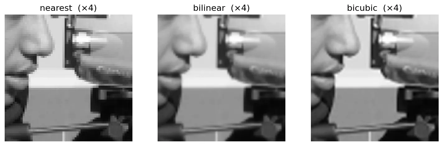

Drag the slider to compare nearest-neighbor and bicubic upsampling of a $96 \times 96$ crop enlarged to $384 \times 384$. Look at the camera’s edges and the face profile.

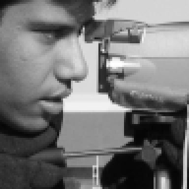
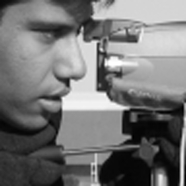NearestBicubic

No interpolation method can create detail that sampling threw away. Thévenaz, Blu and Unser’s review [4] makes the point precisely: the quality of an interpolator is governed by its approximation order and by how closely its kernel approaches the ideal (sinc) reconstructor, and higher-order B-spline methods outperform classic cubic convolution at similar cost. Learned super-resolution, discussed in the Modern view, goes further by hallucinating plausible detail from training data.

Basic relationships between pixels

In plain words: before we can talk about objects in an image, we need rules for which pixels “touch” each other and how far apart two pixels are.

Neighbors of a pixel

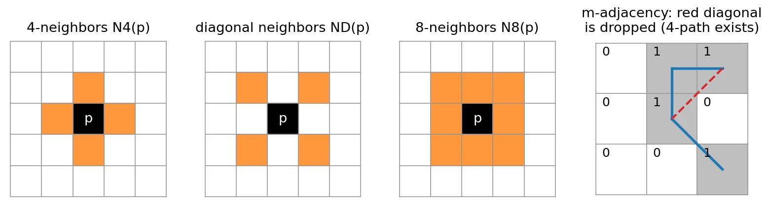
A pixel $p$ at $(x, y)$ has four horizontal and vertical neighbors,

$$N_4(p) = \{(x+1, y),\ (x-1, y),\ (x, y+1),\ (x, y-1)\},$$

four diagonal neighbors,

$$N_D(p) = \{(x+1, y+1),\ (x+1, y-1),\ (x-1, y+1),\ (x-1, y-1)\},$$

and the eight neighbors $N_8(p) = N_4(p) \cup N_D(p)$ [1]. At the image border some neighbors fall outside the image; how we treat them (ignore, pad, reflect) is a choice we meet again in filtering.

Adjacency, connectivity, regions and boundaries

Let $V$ be the set of intensity values that count as “similar” — for a binary image, $V = \{1\}$; for a gray image, perhaps all values between 100 and 120. Two pixels $p$ and $q$ with values in $V$ are [1]:

• 4-adjacent if $q \in N_4(p)$;
• 8-adjacent if $q \in N_8(p)$;
• m-adjacent (mixed) if $q \in N_4(p)$, or $q \in N_D(p)$ and the set $N_4(p) \cap N_4(q)$ contains no pixel whose value is in $V$.

Why m-adjacency? With 8-adjacency, a diagonal step and a two-step “around the corner” route can both connect the same pair of pixels, so paths become ambiguous. m-adjacency keeps a diagonal link only when no 4-connected route exists, which removes the redundant loops (Figure 2.6, right).

A digital path from $p$ to $q$ is a sequence of distinct pixels $(x_0, y_0), \dots, (x_n, y_n)$ with consecutive pixels adjacent; $n$ is the length, and the path is closed if the first and last pixels coincide. Depending on the adjacency used we speak of 4-, 8- or m-paths. For a subset $S$ of pixels, $p$ and $q$ are connected in $S$ if a path between them lies entirely in $S$. The set of pixels connected to $p$ in $S$ is a connected component; if $S$ has only one, it is a connected set.

A connected set is called a region. Two regions are adjacent if their union is connected. The boundary (or border) of a region $R$ is the set of pixels in $R$ that have at least one neighbor outside $R$. Note the difference between a boundary and an edge: a boundary is a global, closed property of a region, while an edge is a local intensity discontinuity that may not close at all (Chapter 10).

The choice of adjacency changes the answer to simple questions such as “how many objects are there?”:

import numpy as np
from skimage.measure import label

b = np.array([[1, 0, 0],
              [0, 1, 0],
              [0, 0, 1]])
print(label(b, connectivity=1).max(),     # 4-connectivity: 3 objects
      label(b, connectivity=2).max())     # 8-connectivity: 1 object

A classic consequence: if the foreground uses 8-connectivity, the background should use 4-connectivity (and vice versa), otherwise a closed digital curve may fail to separate its inside from its outside. This is a basic result of digital topology [1].

Distance measures

For pixels $p = (x, y)$, $q = (u, v)$ and $z$, a function $D$ is a distance metric if $D(p, q) \ge 0$ with equality only when $p = q$, $D(p, q) = D(q, p)$, and $D(p, z) \le D(p, q) + D(q, z)$. Three metrics are standard [1], [5]:

$$\begin{aligned} D_E(p, q) &= \sqrt{(x-u)^2 + (y-v)^2} && \text{(Euclidean)} \\ D_4(p, q) &= |x-u| + |y-v| && \text{(city-block)} \\ D_8(p, q) &= \max(|x-u|,\ |y-v|) && \text{(chessboard)} \end{aligned}$$

The pixels within a fixed $D_E$ of $p$ form a disk; within a fixed $D_4$, a diamond; within a fixed $D_8$, a square. The pixels with $D_4 = 1$ are exactly $N_4(p)$, and those with $D_8 = 1$ are exactly $N_8(p)$. $D_4$ and $D_8$ depend only on coordinates, not on pixel values; a distance along m-paths, by contrast, does depend on the values because the paths do.

import numpy as np
p, q = np.array([2, 3]), np.array([5, 7])
d = np.abs(p - q)
print("D_E =", np.hypot(*d), " D_4 =", d.sum(), " D_8 =", d.max())   # 5.0, 7, 4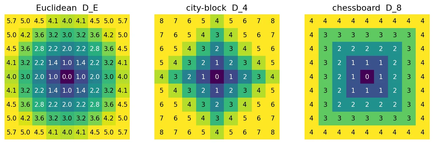

Rosenfeld and Pfaltz [5] introduced efficient two-pass algorithms to compute such distances to the nearest object pixel for every pixel at once — the distance transform, still used for skeletons, morphology and shape matching (Chapter 9).

Introduction to the mathematical tools used in DIP

In plain words: an image is a matrix, so most image processing is arithmetic on matrices. This section lists the operations we will use again and again, and the one property — linearity — that decides which tools apply.

Elementwise versus matrix operations

An elementwise (array) operation acts pixel by pixel. For two $2 \times 2$ images the elementwise product is

$$\begin{bmatrix} a_{11} & a_{12} \\ a_{21} & a_{22} \end{bmatrix} \odot \begin{bmatrix} b_{11} & b_{12} \\ b_{21} & b_{22} \end{bmatrix} = \begin{bmatrix} a_{11}b_{11} & a_{12}b_{12} \\ a_{21}b_{21} & a_{22}b_{22} \end{bmatrix},$$

whereas the matrix product follows row-times-column rules. Unless stated otherwise, image operations — including “multiplying two images” — are elementwise [1]. In NumPy, A * B is elementwise and A @ B is the matrix product.

Linear versus nonlinear operations

Consider an operator $\mathcal{H}$ that maps an input image $f$ to an output $g = \mathcal{H}[f]$. It is linear if

$$\mathcal{H}[a f_1 + b f_2] = a\,\mathcal{H}[f_1] + b\,\mathcal{H}[f_2]$$

for all images $f_1, f_2$ and all constants $a, b$. The two parts of this property are additivity (the output of a sum is the sum of outputs) and homogeneity (scaling the input scales the output). Summing all pixels is linear; taking the maximum is not:

import numpy as np
rng = np.random.default_rng(0)
f1, f2 = rng.random((4, 4)), rng.random((4, 4))
a, b = 2.0, -3.0
print(np.isclose(np.sum(a*f1 + b*f2), a*np.sum(f1) + b*np.sum(f2)))   # True
print(np.isclose(np.max(a*f1 + b*f2), a*np.max(f1) + b*np.max(f2)))   # False

Linearity matters because linear operators are fully described by their response to simple inputs, and a large body of theory (convolution, the Fourier transform, Chapters 3–5) applies to them. Nonlinear operators such as the median filter or morphology can do things linear ones cannot, but are harder to analyze.

Arithmetic operations

Sum, difference, product and quotient of two images of the same size are all elementwise [1]. Three uses stand out.

Averaging noisy images. Suppose we capture $K$ images of a static scene, $g_i(x, y) = f(x, y) + \eta_i(x, y)$, where $f$ is the clean image and $\eta_i$ is noise that is uncorrelated between frames, has zero mean and variance $\sigma^2_\eta$. The average $\bar{g} = \frac{1}{K}\sum_{i=1}^{K} g_i$ satisfies

$$E\{\bar{g}(x, y)\} = f(x, y), \qquad \sigma^2_{\bar{g}}(x, y) = \frac{1}{K}\,\sigma^2_{\eta}(x, y),$$

so the noise standard deviation falls as $1/\sqrt{K}$. Astronomers stack exposures for this reason, and smartphone “night modes” do the same after aligning a burst of frames [7].

import numpy as np
from skimage import data, img_as_float

g = img_as_float(data.camera())
rng = np.random.default_rng(1)
for K in (1, 4, 16, 64):
    avg = np.mean([g + rng.normal(0, 0.2, g.shape) for _ in range(K)], axis=0)
    print(K, round(float(np.std(avg - g)), 3))    # 0.2, 0.1, 0.05, 0.025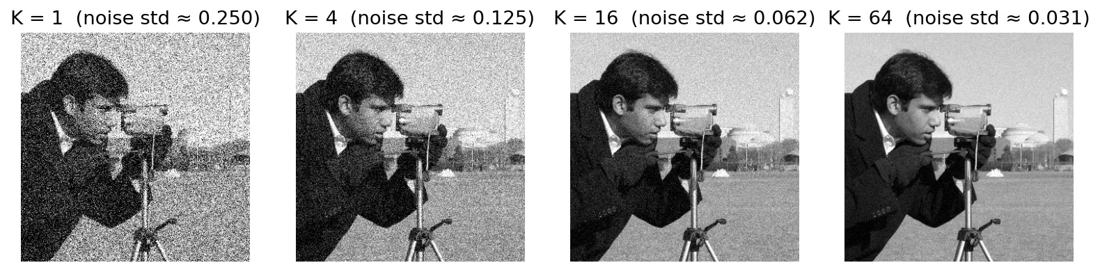

Subtraction reveals differences. Subtracting two frames of a video highlights motion; in medical imaging, subtracting a pre-contrast “mask” image from a post-contrast image leaves mainly the vessels that took up the contrast agent.

Multiplication and division handle shading and masking. If a sensor’s shading pattern $h(x, y)$ is known (for example by imaging a uniform target), the observed image $g = f \cdot h$ can be corrected as $f = g / h$. Multiplying by a binary mask keeps a region of interest and zeroes the rest.

One practical rule: arithmetic results often leave the valid range (differences can be negative, sums can exceed 255). Do the arithmetic in floating point, then rescale. A simple rescaling to $[0, K]$ is $f_m = f - \min f$ followed by $f_s = K\, f_m / \max f_m$.

Set and logical operations

Treat a binary image as a set $A$ of pixel coordinates (the foreground). The usual set operations then apply [1]: union $A \cup B$, intersection $A \cap B$, complement $A^c = \{w \mid w \notin A\}$, and difference $A - B = A \cap B^c$. On binary arrays these become the logical operations OR, AND, NOT and AND-NOT. For gray images, union and intersection are commonly defined as elementwise maximum and minimum. Fuzzy sets generalize this further by letting membership vary between 0 and 1.

import numpy as np
from skimage import data

coins = data.coins()
A = coins > 100                                        # set A: bright pixels
B = np.zeros_like(A); B[:, : coins.shape[1] // 2] = True   # set B: left half
union, inter, diff = A | B, A & B, A & ~B

Set operations are the language of mathematical morphology (Chapter 9) and of combining segmentation masks.

Spatial operations

Spatial operations act directly on pixel values and positions. There are three kinds [1].

Single-pixel operations change each value independently: $s = T(z)$, where $z$ is the input intensity and $s$ the output. The image negative $s = (L-1) - z$ is an example. These are the intensity transformations of Chapter 3.

Neighborhood operations compute each output from a neighborhood $S_{xy}$ around $(x, y)$. Local averaging,

$$g(x, y) = \frac{1}{mn} \sum_{(r, c) \in S_{xy}} f(r, c),$$

where $S_{xy}$ is an $m \times n$ window centered at $(x, y)$, is the simplest; Chapter 3 generalizes it to spatial filtering.

Geometric transformations move pixels. They have two steps: a spatial transformation of coordinates, and intensity interpolation to fill the new grid. The most common family is the affine transform. In homogeneous coordinates,

$$\begin{bmatrix} x' \\ y' \\ 1 \end{bmatrix} = \begin{bmatrix} a_{11} & a_{12} & t_x \\ a_{21} & a_{22} & t_y \\ 0 & 0 & 1 \end{bmatrix} \begin{bmatrix} x \\ y \\ 1 \end{bmatrix},$$

where $(x, y)$ is an input location, $(x', y')$ the output location, the $a_{ij}$ encode rotation, scaling and shear, and $(t_x, t_y)$ is a translation. Affine maps preserve straight lines and parallelism, and chaining several is just multiplying their matrices.

Implementations almost always use inverse mapping: for each output pixel, apply the inverse transform to find where it came from in the input, and interpolate there. Forward mapping (pushing each input pixel to the output) leaves holes and collisions.

import cv2
from skimage import data

img = data.camera()
h, w = img.shape
M = cv2.getRotationMatrix2D(center=(w / 2, h / 2), angle=30, scale=0.8)  # 2x3 affine
rot = cv2.warpAffine(img, M, (w, h), flags=cv2.INTER_LINEAR)  # inverse mapping inside

Image registration

Registration aligns two images of the same scene taken at different times, from different viewpoints or with different sensors. Here the transform is unknown and must be estimated. The classic approach picks tie points (control points) whose positions are known in both images and fits a model to them; for example, a bilinear model

$$x = c_1 v + c_2 w + c_3 v w + c_4, \qquad y = c_5 v + c_6 w + c_7 v w + c_8,$$

maps input coordinates $(v, w)$ to reference coordinates $(x, y)$, and four tie-point pairs give eight equations for the eight unknowns $c_1, \dots, c_8$. Zitová and Flusser’s survey [6] organizes registration into four steps that are still the standard description: feature detection, feature matching, transform model estimation, and resampling.

Vector and matrix operations

A color pixel is a vector, $\mathbf{z} = [z_1, z_2, z_3]^T$ for its red, green and blue values. Vector tools then apply directly; for example, the Euclidean distance from $\mathbf{z}$ to a reference color $\mathbf{a}$,

$$D(\mathbf{z}, \mathbf{a}) = \left[ (\mathbf{z} - \mathbf{a})^T (\mathbf{z} - \mathbf{a}) \right]^{1/2},$$

is the basis of simple color segmentation (Chapter 6). Stacking an $M \times N$ image into an $MN \times 1$ vector also lets any linear operation be written as $\mathbf{g} = \mathbf{H}\mathbf{f}$, a form used in restoration (Chapter 5).

Image transforms

Some problems are easier in a different domain. A 2-D linear transform takes the general form [1]

$$T(u, v) = \sum_{x=0}^{M-1} \sum_{y=0}^{N-1} f(x, y)\, r(x, y, u, v),$$

where $f$ is the input image, $r$ is the forward transformation kernel, and $(u, v)$ are the transform-domain variables. The inverse uses an inverse kernel $s(x, y, u, v)$. When $r(x, y, u, v) = r_1(x, u)\, r_2(y, v)$ the kernel is separable, and the 2-D transform can be done as 1-D transforms along rows and then columns, or in matrix form $\mathbf{T} = \mathbf{A}\mathbf{F}\mathbf{B}$. The Fourier transform (Chapter 4) and the wavelet transforms (Chapter 7) are the two you will meet most.

Probability methods

Intensities can be treated as random quantities. If $n_k$ pixels in an $M \times N$ image have intensity $z_k$, the probability of that intensity is estimated by

$$p(z_k) = \frac{n_k}{MN}, \qquad \sum_{k=0}^{L-1} p(z_k) = 1,$$

which is the normalized histogram. The mean and variance of intensities are

$$m = \sum_{k=0}^{L-1} z_k\, p(z_k), \qquad \sigma^2 = \sum_{k=0}^{L-1} (z_k - m)^2\, p(z_k),$$

where $m$ measures average brightness and $\sigma$ (the standard deviation) measures contrast. Higher moments describe skew and peakedness.

import numpy as np
from skimage import data

img = data.camera()
p = np.bincount(img.ravel(), minlength=256) / img.size   # p(z_k)
z = np.arange(256)
m = np.sum(z * p)
sigma = np.sqrt(np.sum((z - m) ** 2 * p))
print(round(m, 2), round(sigma, 2))                      # 129.06 73.64

Histogram processing (Chapter 3) and noise modeling (Chapter 5) both start here.

Modern view

The fundamentals in this chapter have not been replaced by deep learning; they have become the interface to it. Networks consume sampled, quantized arrays, are trained with losses that encode a model of perception, and are evaluated on data produced by camera pipelines. The reviews below map this territory.

Sampling and interpolation theory. Unser’s “Sampling — 50 years after Shannon” [2] reframes sampling as approximation in shift-invariant spaces: instead of demanding a perfectly band-limited signal and an ideal sinc reconstructor, choose a practical basis (such as B-splines) and project onto it. Its main takeaway is that a good prefilter before sampling and a good reconstruction kernel after it matter more than the exact sampling rate. Thévenaz, Blu and Unser [4] apply this to image interpolation and compare many kernels on equal terms. They show that approximation order and kernel support explain most of the differences, and that B-spline-based interpolation (with a proper prefilter) offers a better quality-for-cost trade-off than Keys’ cubic convolution [3]. Both papers remain the reference point for anyone who implements resizing.

Learned super-resolution. Wang, Chen and Hoi [9] survey deep super-resolution up to about 2019: network designs, upsampling layers placed early or late, loss functions, and benchmarks. Moser et al. [10] extend the picture to transformers and diffusion models and stress open problems such as flexible scale factors and better evaluation. Two works show how the classical ideas survive inside networks. LIIF [11] represents an image as a continuous function queried at any coordinate — a learned interpolator that can upsample by arbitrary factors, including factors not seen in training. Real-ESRGAN [12] tackles the gap between the bicubic downsampling used to create most training pairs and real degradations, by synthesizing training data with a higher-order degradation model that applies blur, noise, resizing and compression more than once. The lesson for this chapter: bicubic interpolation is both the baseline every method is compared against and, through its use in creating training data, a hidden assumption that can make models fail on real images.

Perception and image quality. Wang et al.’s SSIM [13] turned the observations of the perception section — sensitivity to structure and relative change rather than absolute error — into a full-reference quality index that compares local luminance, contrast and structure. Zhai and Min [14] survey the whole field of perceptual quality assessment: full-, reduced- and no-reference methods, and models for specialized content. Deep features changed this area markedly. Zhang et al. [15] collected human similarity judgments and found that distances between deep network features (LPIPS) agree with people far better than PSNR or SSIM, across architectures and training regimes. Ding et al. [16] then asked a sharper question: if you optimize an image-processing network with each quality metric as the loss, which metric gives results people prefer? Their human study shows that rankings on standard quality benchmarks do not reliably predict usefulness as a training objective. In short, Mach bands and the Weber ratio now live inside loss functions.

Camera sensor pipelines. Ramanath et al. [8] describe the classic in-camera pipeline that sits between the sensor array of this chapter and the compressed file you save: demosaicking, white balance, color transforms, gamma, and compression, each a fixed hand-designed stage. Delbracio et al. [7] tour how mobile computational photography reworked this pipeline over two decades, with burst capture, alignment and merging (the averaging-noisy-images idea at scale), and multi-frame super-resolution. Learned replacements now exist for parts or all of it. Chen et al. [17] trained a network to map raw short-exposure sensor data directly to a clean image in very low light, bypassing the traditional pipeline. Ignatov et al. [18] replaced an entire smartphone image signal processor with one network (PyNET) trained to map raw mosaic sensor data to images resembling those from a DSLR.

What did not change? The pixel grid, the bit depth, adjacency and connectivity (still the basis of connected-component labeling in every segmentation post-processing step), affine warps (now differentiable layers inside networks), and histograms. Knowing them is what lets you spot when a model’s input has been resized with the wrong kernel, quantized too coarsely, or compared with a metric that does not match human judgment.

Key takeaways

• Human vision senses relative changes (Weber’s law) and exaggerates edges (Mach bands); perceived brightness depends on the surround. Good image processing respects these facts.
• Images can be formed from any part of the electromagnetic spectrum; for reflected light, $f = i \cdot r$ separates illumination from reflectance.
• Sampling sets spatial resolution, quantization sets intensity resolution, and storage is $M N k$ bits. Too few levels cause false contours in smooth regions.
• Interpolation — nearest, bilinear, bicubic — estimates values between samples; it trades speed for smoothness and sharpness but cannot recover lost detail.
• 4-, 8- and m-adjacency define paths, connected components, regions and boundaries; $D_4$ and $D_8$ are distance metrics whose unit balls are diamonds and squares.
• Image operations are elementwise unless stated otherwise; linearity decides whether convolution and Fourier tools apply.
• Averaging $K$ independent noisy frames reduces noise standard deviation by $\sqrt{K}$; geometric transforms use inverse mapping plus interpolation.
• Deep learning built on these fundamentals: learned interpolators, perceptual losses and learned camera pipelines all inherit this chapter’s concepts.

Exercises

1. A grayscale scanner produces $2400 \times 3300$ images at 12 bits per pixel. How many megabytes does one uncompressed scan need? How many if it is reduced to 8 bits?

Hint

Use $b = M N k$ and divide by $8 \times 10^6$ (or $8 \times 2^{20}$ for MiB). At 12 bits: $2400 \cdot 3300 \cdot 12 / 8 = 11.88$ MB. At 8 bits: 7.92 MB.

2. Quantize skimage.data.moon() to 4, 5 and 6 bits. At which level do false contours disappear for you? Then add a small amount of uniform random noise (amplitude half a quantization step) before quantizing at 4 bits. What changes, and why?

Hint

The noise (called dither) breaks up the large flat steps, so the eye averages the fine noise instead of seeing contours. The mean error stays similar but the visible structure changes — another reminder that squared error and perceived quality differ.

3. In the binary image below, count the connected components of 1-pixels under 4-, 8- and m-connectivity. Then count the components of 0-pixels under 4- and 8-connectivity. Which pairing gives a consistent “inside/outside” answer?

0 0 0 0 0
0 1 1 1 0
0 1 0 1 0
0 1 1 0 0
0 0 0 0 0

Hint

The 1s are a single component under all three adjacencies, but the ring is closed only if diagonal steps count, because of the gap at the lower right. The center 0 is isolated under 4-connectivity (a hole) but joins the outside under 8-connectivity. 4/4 gives an open curve with a hole; 8/8 gives a closed curve without one. Only 8-foreground with 4-background (or the reverse) is consistent. Check your answer with skimage.measure.label.

4. Show that $D_8(p, q) \le D_E(p, q) \le D_4(p, q)$ for any two pixels, and find pixel pairs where each inequality becomes an equality.

Hint

Let $d_x = |x-u|$, $d_y = |y-v|$. Then $\max(d_x, d_y)^2 \le d_x^2 + d_y^2 \le (d_x + d_y)^2$. Equality holds when one of $d_x, d_y$ is zero.

5. Write a function that rotates an image by $\theta$ using forward mapping (push each input pixel to its rounded output position). Display the result for $\theta = 17^\circ$ and explain the holes. Then fix it with inverse mapping and bilinear interpolation.

Hint

Rotation slightly stretches the grid spacing in some directions, so some output pixels receive no input pixel. With inverse mapping, every output pixel asks “where did I come from?” and always gets an answer.

6. You have 10 noisy frames of a static scene with noise standard deviation 12 gray levels. How many frames would you need to bring it below 2 gray levels? What assumption could fail in a real handheld burst, and how do mobile pipelines handle it?

Hint

$12 / \sqrt{K} \lt 2$ requires $K \gt 36$, so 37 frames. The assumption that the scene and camera are static fails; frames must be aligned (registered) before averaging, and moving objects need robust merging [7].

References

1. R. C. Gonzalez and R. E. Woods, Digital Image Processing, 4th ed., Pearson, 2018, Ch. 2. publisher page
2. M. Unser, “Sampling—50 years after Shannon,” Proceedings of the IEEE, vol. 88, no. 4, pp. 569–587, 2000. doi
3. R. Keys, “Cubic convolution interpolation for digital image processing,” IEEE Transactions on Acoustics, Speech, and Signal Processing, vol. 29, no. 6, pp. 1153–1160, 1981. doi
4. P. Thévenaz, T. Blu, and M. Unser, “Interpolation revisited,” IEEE Transactions on Medical Imaging, vol. 19, no. 7, pp. 739–758, 2000. doi
5. A. Rosenfeld and J. L. Pfaltz, “Distance functions on digital pictures,” Pattern Recognition, vol. 1, pp. 33–61, 1968. doi
6. B. Zitová and J. Flusser, “Image registration methods: a survey,” Image and Vision Computing, vol. 21, no. 11, pp. 977–1000, 2003. doi
7. M. Delbracio, D. Kelly, M. S. Brown, and P. Milanfar, “Mobile computational photography: A tour,” arXiv:2102.09000, 2021. arXiv
8. R. Ramanath, W. E. Snyder, Y. Yoo, and M. S. Drew, “Color image processing pipeline,” IEEE Signal Processing Magazine, vol. 22, no. 1, pp. 34–43, 2005. doi
9. Z. Wang, J. Chen, and S. C. H. Hoi, “Deep learning for image super-resolution: A survey,” IEEE Transactions on Pattern Analysis and Machine Intelligence, 2020. arXiv
10. B. Moser, F. Raue, S. Frolov, J. Hees, S. Palacio, and A. Dengel, “Hitchhiker’s guide to super-resolution: Introduction and recent advances,” IEEE Transactions on Pattern Analysis and Machine Intelligence, 2023. arXiv
11. Y. Chen, S. Liu, and X. Wang, “Learning continuous image representation with local implicit image function,” CVPR, 2021. arXiv
12. X. Wang, L. Xie, C. Dong, and Y. Shan, “Real-ESRGAN: Training real-world blind super-resolution with pure synthetic data,” arXiv:2107.10833, 2021. arXiv
13. Z. Wang, A. C. Bovik, H. R. Sheikh, and E. P. Simoncelli, “Image quality assessment: From error visibility to structural similarity,” IEEE Transactions on Image Processing, vol. 13, no. 4, pp. 600–612, 2004. project page
14. G. Zhai and X. Min, “Perceptual image quality assessment: A survey,” Science China Information Sciences, vol. 63, no. 11, 2020. doi
15. R. Zhang, P. Isola, A. A. Efros, E. Shechtman, and O. Wang, “The unreasonable effectiveness of deep features as a perceptual metric,” CVPR, 2018. arXiv
16. K. Ding, K. Ma, S. Wang, and E. P. Simoncelli, “Comparison of full-reference image quality models for optimization of image processing systems,” International Journal of Computer Vision, 2021. arXiv
17. C. Chen, Q. Chen, J. Xu, and V. Koltun, “Learning to see in the dark,” CVPR, 2018. arXiv
18. A. Ignatov, L. Van Gool, and R. Timofte, “Replacing mobile camera ISP with a single deep learning model,” arXiv:2002.05509, 2020. arXiv