Chapter 10 · Image Segmentation I: Edge Detection, Thresholding, and Region Detection

What you’ll learn

• The formal definition of segmentation, and its two families: discontinuity (edges) and similarity (regions).
• How derivatives find points, lines and edges, and how Sobel, Marr–Hildreth (LoG) and Canny work step by step.
• How to link edge pixels into boundaries, including with the Hough transform.
• How Otsu’s method picks a threshold, and what to do when one threshold is not enough.
• How region growing, split-and-merge, k-means, SLIC, normalized cuts, watersheds and motion turn pixels into regions.

The big picture

Until now, most operations took an image and returned an image. Segmentation returns a map of parts: each pixel gets a label saying which object or region it belongs to. Measuring objects, counting cells and reading text all depend on that map.

None of these methods learns from labelled examples. They need no training data, are easy to explain, and their ideas (gradients, hysteresis, between-class variance, graph cuts, flooding) live on inside modern deep pipelines.

Fundamentals

In plain words: segmentation cuts the image into pieces that do not overlap, cover everything, and each look “the same” inside.

Let $R$ be the whole spatial region an image occupies. Segmentation partitions $R$ into $n$ subregions $R_1, \dots, R_n$ such that

$$\begin{aligned} &\text{(a)}\ \textstyle\bigcup_{i=1}^{n} R_i = R, \qquad \text{(b)}\ R_i \text{ is connected},\\ &\text{(c)}\ R_i \cap R_j = \varnothing \ \text{for } i \neq j, \qquad \text{(d)}\ Q(R_i) = \text{TRUE}, \qquad \text{(e)}\ Q(R_i \cup R_j) = \text{FALSE for adjacent } R_i, R_j . \end{aligned}$$

Here $Q$ is a logical predicate: a yes/no test on a set of pixels, for example “all intensities lie within 10 grey levels of each other”. So: every pixel is labelled (a), each region is one connected piece (b), no pixel has two labels (c), each region passes the test (d), and touching regions would fail it if merged (e).

Almost all monochrome segmentation algorithms rest on one of two properties of intensity [1]:

• Discontinuity: boundaries are where intensity changes abruptly. Point, line and edge detection use this.
• Similarity: pixels in one region share a property (intensity, colour, texture). Thresholding, region growing, clustering, graph cuts and watersheds use this.

Edges are precise but often broken; regions are closed by construction but their borders can wander.

Point, line, and edge detection

In plain words: an edge is where brightness changes fast, and “how fast something changes” is exactly what a derivative measures.

Background: derivatives on a pixel grid

For a 1-D digital function $f(x)$ the simplest approximations are

$$\frac{\partial f}{\partial x} \approx f(x+1) - f(x), \qquad \frac{\partial^2 f}{\partial x^2} \approx f(x+1) + f(x-1) - 2f(x).$$

Here $x$ is an integer pixel position and $f(x)$ its intensity. Across a ramp, the first derivative is nonzero all along it, so it gives thick responses. The second derivative is nonzero only at the two ends, with opposite signs, giving a double response with a zero crossing in between, and it reacts far more strongly to fine detail and noise. These facts explain every detector below.

Detecting isolated points

A point is a tiny blob that differs from its surroundings. The Laplacian

$$\nabla^2 f(x, y) = \frac{\partial^2 f}{\partial x^2} + \frac{\partial^2 f}{\partial y^2}$$

is implemented with a $3 \times 3$ kernel whose centre is $-8$ and whose eight neighbours are $1$ (the version that includes diagonals). With $Z(x, y)$ the filtered image, we mark a point wherever $|Z(x, y)| > T$ for a nonnegative threshold $T$. The kernel’s coefficients sum to zero, so flat regions give no response.

Detecting lines

A line is a structure one or a few pixels wide. The Laplacian responds to lines too, but with a double response and no sense of direction. For a specific angle, use a kernel whose $2$s run along that angle and whose other entries are $-1$ (the horizontal one has $2, 2, 2$ in its middle row). Comparing the responses of the horizontal, $+45°$, vertical and $-45°$ kernels tells which orientation dominates at each pixel.

Edge models

Real edges come in three idealized shapes:

• a step edge jumps from one level to another across one pixel (it appears mainly in synthetic images);
• a ramp edge changes linearly over several pixels, which is what blur from optics and sampling produces in real images;
• a roof edge rises and falls back, like a thin line seen through a blur.

On a ramp, the first-derivative magnitude says an edge is present, the sign of the second derivative says which side is bright, and its zero crossing marks the ramp’s centre. But noise too faint to see ruins the second derivative, so smoothing before differentiating is part of every serious edge detector.

Basic edge detection with the gradient

The gradient of $f$ at $(x, y)$ is the vector

$$\nabla f = \begin{bmatrix} g_x \\ g_y \end{bmatrix} = \begin{bmatrix} \partial f / \partial x \\ \partial f / \partial y \end{bmatrix}, \qquad M(x, y) = \sqrt{g_x^2 + g_y^2}, \qquad \alpha(x, y) = \operatorname{atan2}(g_y, g_x).$$

$g_x$ and $g_y$ are the partial derivatives, $M$ is the gradient magnitude (edge strength) and $\alpha$ the gradient direction (where intensity rises fastest); the edge runs perpendicular to $\alpha$. $M$ is often approximated by the cheaper $|g_x| + |g_y|$.

The derivatives are computed with small kernels. The classic operators are summarized in [1]. The Roberts cross operators use $2 \times 2$ diagonal differences. The Prewitt operators use $3 \times 3$ kernels with rows $[-1, 0, 1]$. The Sobel operators weight the centre row by $2$, for example

$$K_x = \begin{bmatrix} -1 & 0 & 1 \\ -2 & 0 & 2 \\ -1 & 0 & 1 \end{bmatrix},$$

a difference in one direction times a $[1, 2, 1]$ smoothing in the other. That built-in smoothing is why Sobel is usually preferred.

import cv2
import numpy as np
from skimage import data

f = data.camera().astype(np.float32) / 255.0
gx = cv2.Sobel(f, cv2.CV_32F, 1, 0, ksize=3)   # d/dx (columns)
gy = cv2.Sobel(f, cv2.CV_32F, 0, 1, ksize=3)   # d/dy (rows)
M = np.hypot(gx, gy)                           # gradient magnitude
alpha = np.arctan2(gy, gx)                     # gradient direction, radians
edges = M > 0.3 * M.max()                      # crude thresholded edge map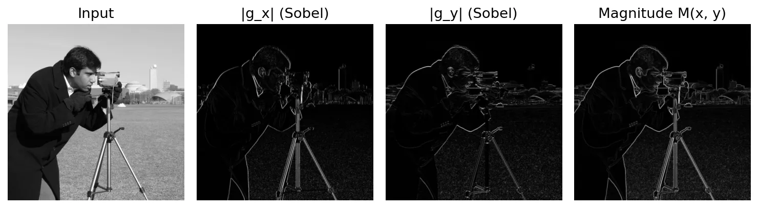

Try the Sobel kernel yourself. Swap it to the $y$ version, or change the $2$s to $1$s to get Prewitt, and watch the response change.

Kernel playgroundEdit any cell or pick a preset. The output updates as you type.

Thresholding $M$ gives a poor edge map: thick edges, lost weak edges, and clutter from texture. The next two detectors build smoothing and thinning into the design.

The Marr–Hildreth edge detector

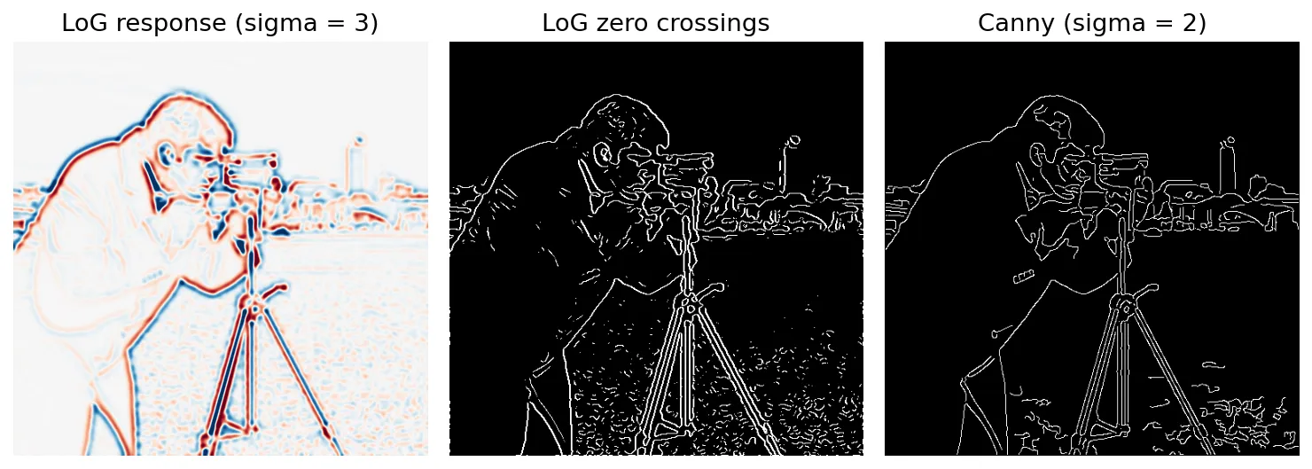
Marr and Hildreth [2] argued that intensity changes occur at many scales, so a detector needs an adjustable size, and that second-derivative zero crossings mark edge centres. Their operator is the Laplacian of a Gaussian (LoG), $\nabla^2 G$, where

$$G(x, y) = e^{-\frac{x^2 + y^2}{2\sigma^2}}, \qquad \nabla^2 G(x, y) = \frac{x^2 + y^2 - 2\sigma^2}{\sigma^4}\, e^{-\frac{x^2 + y^2}{2\sigma^2}}.$$

$\sigma$ is the Gaussian’s standard deviation and sets the scale (larger $\sigma$, only coarser edges survive); the normalizing constant is dropped since only zero crossings matter. Its shape earns $\nabla^2 G$ the name Mexican hat. The algorithm:

1. Smooth with an $n \times n$ Gaussian, $n$ the smallest odd integer $\geq 6\sigma$.
2. Take the Laplacian of the result (by linearity, steps 1–2 are one convolution with $\nabla^2 G$).
3. Mark zero crossings: pixels where some pair of opposite neighbours has different signs and an absolute difference above a threshold; without the threshold, every ripple in a flat area becomes an “edge”.

A difference of Gaussians (DoG), $G_{\sigma_1} - G_{\sigma_2}$ with $\sigma_1 / \sigma_2 \approx 1.6$, approximates the LoG [1]. Zero crossings form closed contours, but they produce “spaghetti” in texture and round off corners.

The Canny edge detector

Canny [3] turned edge detection into an optimization problem with three criteria:

1. Low error rate: find all true edges and no spurious ones.
2. Good localization: the detected edge should be as close as possible to the true edge.
3. Single response: one true edge should produce one detected edge, not a double line.

For a 1-D step in white noise, the optimal filter is well approximated by the first derivative of a Gaussian. The practical 2-D algorithm follows:

1. Smooth the image with a Gaussian of standard deviation $\sigma$: $f_s = G_\sigma \star f$.
2. Compute the gradient magnitude $M$ and angle $\alpha$ of $f_s$.
3. Non-maximum suppression. Quantize $\alpha$ into four directions. Zero any pixel whose $M$ is smaller than either neighbour along the gradient direction. Ridges become one pixel thick.
4. Double thresholding. Pick $T_H$ and $T_L$ with $T_H / T_L$ about $2$ to $3$ [1]. Pixels above $T_H$ are strong; pixels between are weak.
5. Hysteresis. Keep a weak pixel only if it connects, through weak pixels, to a strong one.

Hysteresis is the key idea. One threshold either breaks contours or admits noise; two thresholds plus connectivity keep faint contours anchored to strong ones and drop isolated weak responses.

import cv2
from scipy import ndimage as ndi
from skimage import data, feature

f8 = data.camera()
canny_cv = cv2.Canny(cv2.GaussianBlur(f8, (0, 0), 2), 30, 90)      # uint8 0/255
canny_sk = feature.canny(f8 / 255.0, sigma=2, low_threshold=0.05, high_threshold=0.15)
log = ndi.gaussian_laplace(f8 / 255.0, sigma=3)                   # Marr-Hildreth steps 1-2

cv2.Canny has no smoothing parameter, so we blur first; scikit-image takes sigma directly.

Drag the slider to see which structures Canny keeps (edges are shown dark on white).

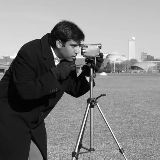
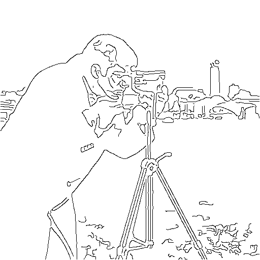InputCanny σ=2

Linking edge points

Even Canny leaves gaps. Edge linking assembles edge pixels into meaningful boundaries.

Local processing. In a small neighbourhood $S_{xy}$ of each edge pixel $(x, y)$, link a neighbour $(s, t)$ if both magnitude and angle are similar:

$$|M(s, t) - M(x, y)| \leq E, \qquad |\alpha(s, t) - \alpha(x, y)| \leq A,$$

where $E$ and $A$ are positive tolerances. A cheaper variant thresholds $M$, keeps pixels whose angle is near a desired direction, and fills short gaps along each row; rotating the image handles other directions.

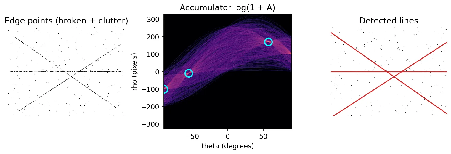
Global processing with the Hough transform. When the shape is known, let every edge pixel vote for all shapes that could pass through it. For lines, Duda and Hart [4] proposed the normal representation

$$\rho = x \cos\theta + y \sin\theta ,$$

where $\theta$ is the angle of the line’s normal and $\rho$ its signed distance from the origin; unlike slope–intercept, this stays bounded for vertical lines. Each point $(x_k, y_k)$ becomes a sinusoid in the $\rho\theta$ plane, and the sinusoids of collinear points meet in one cell. The algorithm:

1. Compute a binary edge map (e.g. Canny).
2. Quantize the $\rho\theta$ plane into accumulator cells $A(\rho, \theta)$, all zero.
3. For each edge pixel and each $\theta$, compute $\rho$ and increment $A(\rho, \theta)$.
4. Local maxima with large counts are lines; optionally check the continuity of their voters to get segments.

# continues from the Canny snippet above (uses cv2, np and canny_cv)
import numpy as np

lines = cv2.HoughLines(canny_cv, rho=1, theta=np.pi / 180, threshold=120)
for rho, theta in lines[:5, 0]:
    print(f"rho = {rho:6.1f} px, theta = {np.degrees(theta):5.1f} deg")

OpenCV reports $\theta \in [0°, 180°)$ with signed $\rho$, the same convention over a different range. Voting extends to circles and other shapes with more parameters.

Thresholding

In plain words: pick a grey level; everything brighter is “object” and everything darker is “background”. The art is in picking the level.

Foundation

Given an intensity threshold $T$, global thresholding produces

$$g(x, y) = \begin{cases} 1 & \text{if } f(x, y) > T \\ 0 & \text{otherwise.} \end{cases}$$

A constant $T$ is a global threshold; one that changes with position is variable (local, adaptive); several thresholds give multiple thresholding. It works when the histogram has well separated modes. Noise widens the modes, uneven illumination and reflectance shift them, and a tiny object makes a bump that is easy to miss.

Basic global thresholding

An easy iterative rule works well when the modes are clearly separated:

1. Pick an initial $T$, such as the mean intensity.
2. Split the pixels into $G_1$ (values $> T$) and $G_2$ (values $\leq T$).
3. Compute the mean of each group, $m_1$ and $m_2$.
4. Set $T = \tfrac{1}{2}(m_1 + m_2)$.
5. Repeat 2–4 until $T$ changes by less than a small $\Delta T$.

def basic_global(img, dT=0.5):
    T = img.mean()
    while True:
        m1, m2 = img[img > T].mean(), img[img <= T].mean()
        T_new = 0.5 * (m1 + m2)
        if abs(T_new - T) < dT:
            return T_new
        T = T_new

Otsu’s optimum global thresholding

Otsu [5] picks the threshold that makes the two classes most separable, measured by the between-class variance. It needs only the histogram.

Let the image have $L$ levels, $n_i$ pixels at level $i$ and $MN$ pixels in total, so the normalized histogram is $p_i = n_i / MN$. A threshold $k$ splits the levels into $C_1 = [0, k]$ and $C_2 = [k+1, L-1]$. Define

$$P_1(k) = \sum_{i=0}^{k} p_i, \qquad m(k) = \sum_{i=0}^{k} i\, p_i, \qquad m_G = \sum_{i=0}^{L-1} i\, p_i ,$$

where $P_1(k)$ is the probability that a pixel falls in $C_1$, $m(k)$ is the cumulative mean up to level $k$, and $m_G$ is the global mean. Then $P_2 = 1 - P_1$, and the class means are $m_1 = m / P_1$ and $m_2 = (m_G - m)/P_2$.

Derivation. The global mean is $m_G = P_1 m_1 + P_2 m_2$. The between-class variance is the weighted spread of the class means around it:

$$\sigma_B^2 = P_1 (m_1 - m_G)^2 + P_2 (m_2 - m_G)^2 .$$

Substitute $m_G = P_1 m_1 + P_2 m_2$. Then $m_1 - m_G = P_2 (m_1 - m_2)$ and $m_2 - m_G = P_1 (m_2 - m_1)$, so

$$\sigma_B^2 = P_1 P_2^2 (m_1 - m_2)^2 + P_2 P_1^2 (m_1 - m_2)^2 = P_1 P_2 (m_1 - m_2)^2 .$$

The farther apart the class means, the larger $\sigma_B^2$. Substituting $m_1 = m/P_1$ and $m_2 = (m_G - m)/(1-P_1)$ gives a form that needs only cumulative sums:

$$\sigma_B^2(k) = \frac{\big(m_G P_1(k) - m(k)\big)^2}{P_1(k)\,\big(1 - P_1(k)\big)} .$$

The optimum is $k^\ast = \arg\max_k \sigma_B^2(k)$ (average ties). Since the global variance $\sigma_G^2$ is the sum of between- and within-class variance and does not depend on $k$, this also minimizes the within-class variance. The ratio

$$\eta = \frac{\sigma_B^2(k^\ast)}{\sigma_G^2}, \qquad 0 \le \eta \le 1,$$

measures separability: near $1$ for two clean modes, lower when they overlap.

import numpy as np
from skimage import data, filters

def otsu(img):
    p = np.bincount(img.ravel(), minlength=256) / img.size   # normalized histogram
    P1 = np.cumsum(p)                                         # class-1 probability
    m = np.cumsum(np.arange(256) * p)                         # cumulative mean
    mG = m[-1]                                                # global mean
    with np.errstate(divide="ignore", invalid="ignore"):
        sB2 = (mG * P1 - m) ** 2 / (P1 * (1 - P1))
    sB2 = np.nan_to_num(sB2)
    k = int(np.argmax(sB2))
    return k, sB2[k] / np.var(img)                            # threshold, separability

coins = data.coins()
k, eta = otsu(coins)          # k = 107, eta ≈ 0.76
assert k == filters.threshold_otsu(coins)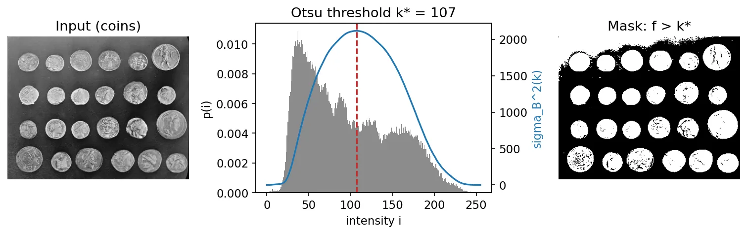

Using smoothing and edges to improve thresholding

• Smooth first. Noise widens the modes until they merge; smoothing narrows them again, as long as the object is large compared with the filter.
• Use only pixels near edges. A small object’s mode is buried under the background’s. Keep pixels where an edge indicator (gradient magnitude or $|\nabla^2 f|$) is high, say above its 99.7th percentile, and compute the histogram from those pixels only. They lie roughly half on each side of a boundary, so the histogram becomes balanced and bimodal. Apply the resulting threshold to the whole image.

Multiple thresholds

Otsu’s criterion generalizes to $K$ classes separated by $K-1$ thresholds:

$$\sigma_B^2 = \sum_{k=1}^{K} P_k (m_k - m_G)^2 ,$$

with $P_k$ and $m_k$ the probability and mean of class $k$, found by exhaustive search. skimage.filters.threshold_multiotsu(coins, classes=3) returns [77, 139].

Variable thresholding

When illumination varies, no single $T$ works. Three remedies:

1. Partitioning. Threshold each tile with its own Otsu value; each tile must contain both classes.
2. Local properties. With $m_{xy}$ and $\sigma_{xy}$ the mean and standard deviation in a window around $(x, y)$, use $T_{xy} = a\,\sigma_{xy} + b\,m_{xy}$ ($a, b \ge 0$), or more generally a predicate $Q(\sigma_{xy}, m_{xy})$. Sauvola and Pietikäinen’s document rule [7], $T_{xy} = m_{xy}\big(1 + k(\sigma_{xy}/R - 1)\big)$ with $R$ the dynamic range of $\sigma$ and small $k > 0$, belongs to this family.
3. Moving averages. For text, scan in a zigzag and threshold each pixel at $c \cdot m(k)$, where $m(k)$ is the mean of the last $n$ pixels and $c$ is slightly below $1$.

from skimage import data, filters

page = data.page()
global_mask = page > filters.threshold_otsu(page)
local_T = filters.threshold_local(page, block_size=35, offset=10)  # Gaussian-weighted local mean - 10
local_mask = page > local_T
sauvola_mask = page > filters.threshold_sauvola(page, window_size=25, k=0.2)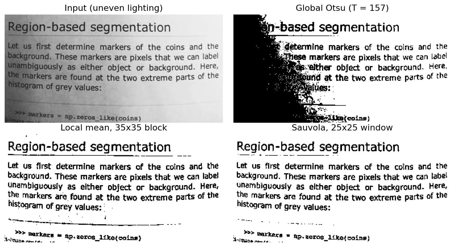

Region growing, splitting, and merging

In plain words: start from a few “seed” pixels and keep adding neighbours that look like them; or start from the whole image and keep cutting it into four until every piece is uniform.

Region growing

Region growing adds to each seed the neighbouring pixels that satisfy a similarity predicate. Choose the seeds (by hand, by a safe threshold, or from histogram peaks), the predicate (e.g. $|f(x, y) - f(\text{seed})| \leq T$, or a test on region statistics), the connectivity (4 or 8), and the stopping rule (no neighbour passes; size or shape limits make it more robust).

from collections import deque
import numpy as np

def region_grow(img, seed, tol):
    """Grow from `seed` over 8-connected pixels whose value is within `tol` of the seed value."""
    H, W = img.shape
    ref = float(img[seed])
    mask = np.zeros((H, W), bool)
    mask[seed] = True
    q = deque([seed])
    while q:
        r, c = q.popleft()
        for dr in (-1, 0, 1):
            for dc in (-1, 0, 1):
                rr, cc = r + dr, c + dc
                if 0 <= rr < H and 0 <= cc < W and not mask[rr, cc] \
                        and abs(float(img[rr, cc]) - ref) <= tol:
                    mask[rr, cc] = True
                    q.append((rr, cc))
    return mask

skimage.segmentation.flood(img, seed, tolerance=tol) does the same in compiled code.

Region splitting and merging with quadtrees

Instead of seeds, start with the whole image $R$ and a predicate $Q$:

1. Split any region $R_i$ for which $Q(R_i) = \text{FALSE}$ into four equal quadrants.
2. Repeat until every region passes $Q$, or the region reaches a minimum size.
3. Merge any two adjacent regions $R_j, R_k$ for which $Q(R_j \cup R_k) = \text{TRUE}$.
4. Stop when no more splits or merges are possible.

Splitting is stored as a quadtree: the root is the image, each node has four children. Splitting alone gives blocky regions; merging lets regions cross quadrant borders. A typical predicate: “standard deviation above $a$ and mean between $b$ and $c$”.

Region segmentation using clustering and superpixels

In plain words: treat every pixel as a point described by a few numbers (its colour, maybe its position) and gather nearby points into groups.

k-means clustering

Represent each pixel by a feature vector $\mathbf{z} \in \mathbb{R}^n$, for example its Lab colour ($n = 3$). k-means looks for $k$ cluster centres $\mathbf{m}_1, \dots, \mathbf{m}_k$ and sets $C_1, \dots, C_k$ that minimize

$$J = \sum_{i=1}^{k} \sum_{\mathbf{z} \in C_i} \lVert \mathbf{z} - \mathbf{m}_i \rVert^2 ,$$

the total squared distance to the cluster means. The global minimum is NP-hard to find, so the standard algorithm alternates: assign each vector to its nearest centre, then move each centre to the mean of its vectors. It reaches a local minimum, so run it from several starts. Clustering on colour alone ignores position, so one cluster can be scattered over the image.

Superpixels and SLIC

A superpixel is a small, compact group of similar connected pixels. A few hundred superpixels instead of $10^5$ pixels shrink later problems without moving important boundaries. SLIC by Achanta et al. [8] is k-means in the 5-D space $[l, a, b, x, y]$. With $N$ pixels and $K$ superpixels, the grid spacing is $S = \sqrt{N / K}$.

1. Place $K$ centres on a grid of spacing $S$, each nudged to the lowest gradient in its $3 \times 3$ neighbourhood.
2. Search only a $2S \times 2S$ window around each centre and assign pixels by

$$D = \sqrt{d_c^2 + \left(\frac{d_s}{S}\right)^2 m^2 },$$

where $d_c$ and $d_s$ are Euclidean distances in Lab colour and in $(x, y)$, and $m$ is the compactness: large $m$ gives square-ish superpixels, small $m$ hugs colour edges. 3. Move each centre to the mean of its pixels; repeat about ten times. 4. Enforce connectivity by merging stray fragments into a neighbour.

The local search makes each iteration $O(N)$, independent of $K$.

from skimage import data, segmentation

img = data.astronaut()
sp = segmentation.slic(img, n_segments=300, compactness=10, start_label=1)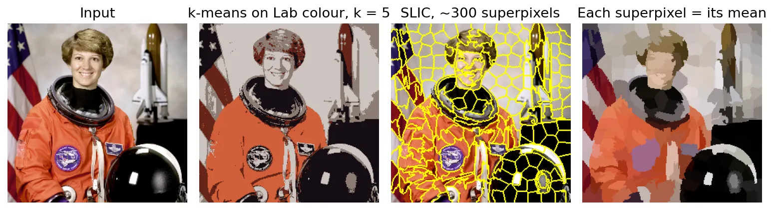

Region segmentation using graph cuts

In plain words: draw the image as a net in which neighbouring pixels are tied together by strings, strong strings for similar pixels and weak strings for different ones. Segmenting is cutting the net into pieces while snapping only weak strings.

Images as graphs

A graph $G = (V, E)$ has nodes $V$ and edges $E$. Each pixel (or superpixel) is a node; nearby nodes are joined by an edge with a nonnegative similarity weight $w(i, j)$, for example

$$w(i, j) = \exp\!\left(-\frac{\lVert \mathbf{F}_i - \mathbf{F}_j \rVert^2}{\sigma_I^2}\right) \exp\!\left(-\frac{\lVert \mathbf{X}_i - \mathbf{X}_j \rVert^2}{\sigma_X^2}\right) \ \text{ if } \lVert \mathbf{X}_i - \mathbf{X}_j \rVert \le r, \text{ else } 0,$$

where $\mathbf{F}$ is a feature vector (intensity, colour), $\mathbf{X}$ a spatial position, $\sigma_I$ and $\sigma_X$ scale parameters, and $r$ a radius that keeps the graph sparse.

Minimum graph cuts

A cut splits $V$ into two disjoint sets $A$ and $B$ by removing the edges between them. Its cost is

$$\operatorname{cut}(A, B) = \sum_{u \in A,\, v \in B} w(u, v).$$

The minimum cut removes as little similarity as possible. A popular formulation adds a source node (object) and a sink node (background), linked to every pixel with weights saying how much it resembles each. A minimum source–sink cut labels every pixel and can be found efficiently with maximum-flow algorithms; it underlies interactive tools where a user scribbles a few object and background pixels.

Normalized cuts

Without source and sink, a plain minimum cut prefers to cut off a single node or tiny group, because few edges are removed. Shi and Malik [9] fixed this with the normalized cut

$$\operatorname{Ncut}(A, B) = \frac{\operatorname{cut}(A, B)}{\operatorname{assoc}(A, V)} + \frac{\operatorname{cut}(A, B)}{\operatorname{assoc}(B, V)}, \qquad \operatorname{assoc}(A, V) = \sum_{u \in A,\, t \in V} w(u, t),$$

the total connection from $A$ to all nodes. A tiny $A$ has a tiny $\operatorname{assoc}$, so cutting it off is now expensive. Exact minimization is NP-hard, but a relaxation gives an eigenproblem; with $W$ the weight matrix and $D$ the diagonal matrix of degrees $d_i = \sum_j w(i, j)$,

$$(D - W)\, \mathbf{y} = \lambda D\, \mathbf{y}.$$

The eigenvector of the second smallest eigenvalue is a soft partition indicator; thresholding it splits the graph, and recursion gives more segments. Practical code runs it on a superpixel graph.

import numpy as np
from skimage import data, segmentation, graph

img = data.coffee()
sp = segmentation.slic(img, n_segments=400, compactness=30, start_label=1)
rag = graph.rag_mean_color(img, sp, mode="similarity")   # edge weight = exp(-|c_i - c_j|^2 / sigma)
ncut = graph.cut_normalized(sp, rag, rng=0)              # recursive two-way Ncut
print(sp.max(), "superpixels ->", len(np.unique(ncut)), "regions")

Segmentation using morphological watersheds

In plain words: think of the image as a landscape where bright means high. Pour water in from every valley; where water from two valleys is about to meet, build a wall. The walls are the segmentation.

Background: basins and dams

Treat intensity as height. Each regional minimum has a catchment basin, the points whose water drains to it; watershed lines separate basins. We usually flood the gradient magnitude, not the image: interiors are low, boundaries are ridges, so each basin is one object.

A dam uses Chapter 9’s morphology. When two flooded components are about to merge, dilate both with a $3 \times 3$ structuring element, restricted to pixels below the current level; pixels reached by both in the same step become dam pixels, set higher than the image maximum. The dams are one pixel thick and connected.

The watershed algorithm

Let $M_1, \dots, M_R$ be the regional minima of an image $g$, let $\min$ and $\max$ be its extreme values, and let $T[n] = \{(s, t) : g(s, t) < n\}$ be the set of pixels below level $n$. Let $C[n]$ be the union of the flooded parts of all catchment basins at level $n$. Flooding proceeds for $n = \min + 1, \dots, \max + 1$. Start with $C[\min + 1] = T[\min + 1]$. At each level, take each connected component $q$ of $T[n]$ and compare it with $C[n-1]$:

1. $q \cap C[n-1]$ is empty: a new minimum has appeared; $q$ becomes a new basin.
2. $q \cap C[n-1]$ contains one component of $C[n-1]$: $q$ lies inside one existing basin; add it.
3. $q \cap C[n-1]$ contains two or more components: two basins are meeting; build a dam inside $q$ as above.

Vincent and Soille [10] gave the efficient implementation used today: sort pixels by height, then flood level by level with a FIFO queue (“immersion simulation”).

The use of markers

On a raw gradient the watershed over-segments: noise and texture create thousands of minima. The cure is markers, components known in advance to be inside objects (internal) or background (external). Flooding starts only from markers, so there are as many regions as markers. Markers come from safe thresholds, smoothed minima, distance-transform peaks, or user clicks.

import numpy as np
from scipy import ndimage as ndi
from skimage import data, filters, morphology, segmentation

coins = data.coins()
elevation = filters.sobel(coins.astype(float))
markers = np.zeros_like(coins, dtype=np.int32)
markers[coins < 30] = 1        # sure background
markers[coins > 150] = 2       # sure object
ws = segmentation.watershed(elevation, markers)
coins_mask = morphology.remove_small_objects(ndi.binary_fill_holes(ws == 2), 100)
labels, n = ndi.label(coins_mask)   # n = 24 coins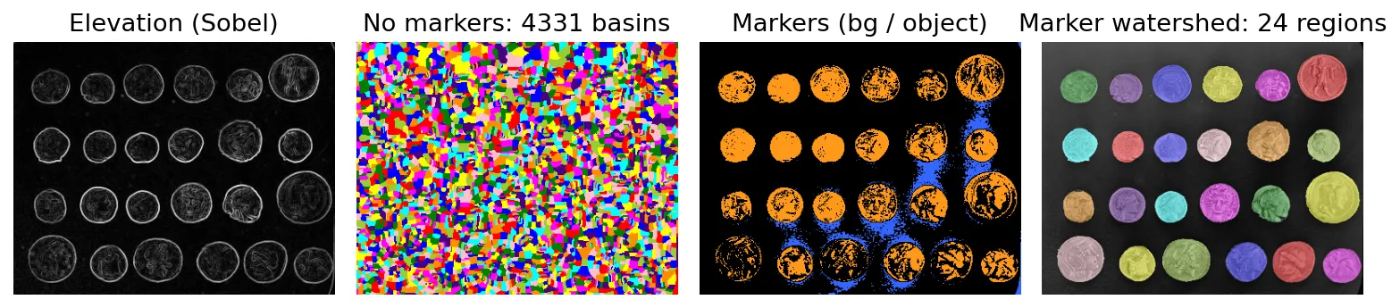

The use of motion in segmentation

In plain words: if the camera is still, the things that moved between two frames are the things you care about. Subtract the frames and the moving objects light up.

Spatial techniques: difference images

Given two frames $f(x, y, t_i)$ and $f(x, y, t_j)$ of a static scene with a static camera, the difference image is

$$d_{ij}(x, y) = \begin{cases} 1 & \text{if } |f(x, y, t_i) - f(x, y, t_j)| > T \\ 0 & \text{otherwise,} \end{cases}$$

with $T$ just above the noise level. Noise specks are removed by discarding small connected components.

Accumulative differences

One difference shows a moving object twice: where it was and where it is. An accumulative difference image (ADI) compares a reference frame $R = f(x, y, t_1)$ with each later frame and counts:

$$\begin{aligned} A_k &= A_{k-1} + 1 \ \text{ if } |R - f_k| > T, \\ P_k &= P_{k-1} + 1 \ \text{ if } R - f_k > T, \\ N_k &= N_{k-1} + 1 \ \text{ if } R - f_k < -T, \end{aligned}$$

each unchanged otherwise and starting at zero ($f_k = f(x, y, t_k)$). For an object brighter than the background, the positive ADI $P$ marks where the object was in the reference frame; the negative ADI grows in the direction of motion, at a rate set by the speed; the absolute ADI $A$ contains both.

import numpy as np

def accumulative_differences(frames, T):
    R = frames[0].astype(float)
    A = np.zeros(R.shape, int); P = np.zeros(R.shape, int); N = np.zeros(R.shape, int)
    for f in frames[1:]:
        d = R - f.astype(float)
        A += np.abs(d) > T
        P += d > T
        N += d < -T
    return A, P, N

Building a reference image

A reference with no moving objects is rare. Once the positive ADI shows that an object has fully left its initial location, copy those pixels from the current frame into the reference; doing this for every mover gives a background reference image. Background subtraction methods extend this idea with per-pixel statistical models.

Modern view

Five surveys map the field; below each is what deep learning did and did not change.

Classical thresholding. Sezgin and Sankur [6] sort thresholding methods into six families by the information they exploit (histogram shape, measurement-space clustering, entropy, object attributes, spatial correlation, local grey-level surface) and evaluate forty of them on non-destructive testing and document images, singling out those that perform consistently in both. Otsu’s method sits in the clustering family.

Deep segmentation. Minaee et al. [11] survey deep semantic and instance segmentation, grouping models into fully convolutional networks, encoder–decoders, multi-scale and pyramid models, recurrent networks, attention models and adversarial generative models, and reviewing datasets and results. The landmark designs echo classical ideas:

• FCN [13] made classification networks fully convolutional so they output a label map, fusing coarse deep features with fine shallow ones: learned multi-scale analysis.
• U-Net [14] added a symmetric expanding path with skip connections, giving precise boundaries from little training data, and became a default in biomedical imaging.
• DeepLab [16] used atrous convolution and atrous spatial pyramid pooling for resolution and context, plus a fully connected CRF to sharpen boundaries.
• Mask R-CNN [15] added a mask branch to an object detector, separating touching objects of one class, the job markers did for the watershed.

Foundation models and promptable segmentation. Segment Anything (SAM) [17] is a model prompted with points, boxes or masks, trained on SA-1B, over one billion masks on 11 million images. Click-in, mask-out is the interface of seeded region growing and interactive graph cuts, with learned instead of hand-made similarity. Zhou et al. [12] review over 300 methods of this “foundation model era”, split into generic tasks (semantic, instance, panoptic) and promptable ones (interactive, referring, few-shot), and show how large pretrained models carry segmentation knowledge.

Edge detection. Sun et al. [18] group traditional edge detectors into gradient, Gaussian-difference, multi-scale and structured-learning methods, and deep ones into encoder–decoder, network-reconstruction and multi-scale fusion designs. HED [19], the key early deep design, fuses side outputs from several network depths into one edge map, a learned heir to Marr and Hildreth’s multi-scale argument. The survey concludes that learned detectors now perform close to, or beyond, human level on standard benchmarks, leaving lightweight models, weak supervision and interpretability as open problems.

Superpixels. Stutz, Hermans and Leibe [20] benchmark 28 algorithms, stressing tuned parameters and strictly enforced connectivity, with metrics independent of the number of superpixels and robustness tests against noise, blur and affine transforms.

What changed and what did not. Learned features replaced hand-designed predicates and edge strengths, dramatically so on natural images. The classical skeleton remains: network outputs are probability maps that get thresholded; touching instances still need separating, by boxes, learned markers or a watershed on a predicted distance map; and Otsu, Canny and Hough still win where data are scarce, compute is tight or behaviour must be predictable, as in document scanning and industrial inspection.

Key takeaways

• Segmentation partitions an image into connected, non-overlapping regions that each satisfy a predicate $Q$; methods look either for discontinuities (edges) or for similarity (regions).
• First derivatives give thick edge responses; second derivatives give double responses with a zero crossing at the edge centre and are very sensitive to noise, so smooth before differentiating.
• Canny = Gaussian smoothing + gradient + non-maximum suppression + double threshold with hysteresis; the last step is what keeps faint but connected edges.
• The Hough transform turns line finding into voting in $(\rho, \theta)$ space, which is robust to gaps and clutter.
• Otsu’s threshold maximizes the between-class variance $\sigma_B^2 = P_1 P_2 (m_1 - m_2)^2$, computable from cumulative histogram sums; use local thresholds when lighting is uneven.
• Region methods (growing, split-and-merge, k-means, SLIC, normalized cuts) group by similarity; normalized cuts avoid the small-segment bias of plain minimum cuts.
• The watershed floods a gradient image from its minima and builds dams where floods meet; markers are essential to avoid over-segmentation.
• Deep networks learned the similarity and edge measures, but thresholding, multi-scale fusion, seeds or prompts, and instance separation are still the skeleton of modern pipelines.

Exercises

1. A 1-D signal is flat at 10 for five samples, rises linearly to 50 over four samples, then stays at 50. Write down its first and second differences, and mark where the zero crossing of the second difference lies relative to the ramp.

Hint

The first difference is 10 on the four ramp steps, 0 elsewhere. The second difference is +10 at the ramp’s start, −10 at its end, 0 between, so the zero crossing lies mid-ramp.

2. Show that maximizing the between-class variance $\sigma_B^2$ is equivalent to minimizing the weighted within-class variance $\sigma_W^2 = P_1 \sigma_1^2 + P_2 \sigma_2^2$.

Hint

Split $\sum_i (i - m_G)^2 p_i$ at $k$ and add and subtract each class mean; cross terms vanish, leaving $\sigma_G^2 = \sigma_W^2 + \sigma_B^2$, with $\sigma_G^2$ independent of $k$.

3. In Canny’s detector, what happens if you set $T_L = T_H$? What if $T_L = 0$? Predict the result, then test with skimage.feature.canny on data.camera().

Hint

$T_L = T_H$ disables hysteresis: broken contours. $T_L = 0$ keeps every thinned pixel connected to a strong edge, so edges leak into the grass texture.

4. A Hough accumulator uses $\theta$ in 1° steps over $[-90°, 90°)$ and $\rho$ in 1-pixel steps for a $640 \times 480$ image. How many accumulator cells are there, and how many increments does an edge map with 20,000 edge pixels cause?

Hint

$|\rho| \le \sqrt{640^2 + 480^2} = 800$, so about 1,601 $\rho$ bins and 180 $\theta$ bins, which is about 288,000 cells. Each edge pixel votes once per $\theta$: $20{,}000 \times 180 = 3.6$ million increments.

5. Explain why plain minimum cut tends to isolate single pixels, using a 4-connected pixel graph with uniform weights $w$. Then compute Ncut for isolating one interior pixel in an $N$-pixel image and show that it is close to 1, whereas a balanced cut along a short boundary scores close to 0.

Hint

Isolating one pixel costs $4w$, less than any long boundary. For Ncut, $\operatorname{assoc}(A, V) = 4w$, so the first term is $1$ and the second is tiny: Ncut ≈ 1, a bad score.

6. Run the marker-controlled watershed on data.coins() with background markers at coins < 30 and object markers at coins > 150, as above, then change the object threshold to 120, 190 and 230. Which coins merge or vanish, and why?

Hint

At 120, object markers land on the bright top band, so coins merge with the background into big regions (we counted 11). At 190 there are still 24, since one marker pixel per coin suffices; at 230 darker coins lose their markers and vanish (13 left). Markers decide the result.

References

1. R. C. Gonzalez and R. E. Woods, Digital Image Processing, 4th ed., Pearson, 2018, Ch. 10. publisher page
2. D. Marr and E. Hildreth, “Theory of edge detection,” Proceedings of the Royal Society of London. Series B, vol. 207, no. 1167, pp. 187–217, 1980. doi
3. J. Canny, “A Computational Approach to Edge Detection,” IEEE Transactions on Pattern Analysis and Machine Intelligence, vol. PAMI-8, no. 6, pp. 679–698, 1986. doi
4. R. O. Duda and P. E. Hart, “Use of the Hough transformation to detect lines and curves in pictures,” Communications of the ACM, vol. 15, pp. 11–15, 1972. doi
5. N. Otsu, “A Threshold Selection Method from Gray-Level Histograms,” IEEE Transactions on Systems, Man, and Cybernetics, vol. 9, no. 1, pp. 62–66, 1979. doi
6. M. Sezgin and B. Sankur, “Survey over image thresholding techniques and quantitative performance evaluation,” Journal of Electronic Imaging, vol. 13, no. 1, pp. 146–165, 2004. doi
7. J. Sauvola and M. Pietikäinen, “Adaptive document image binarization,” Pattern Recognition, vol. 33, no. 2, pp. 225–236, 2000. doi
8. R. Achanta, A. Shaji, K. Smith, A. Lucchi, P. Fua and S. Süsstrunk, “SLIC Superpixels Compared to State-of-the-Art Superpixel Methods,” IEEE Transactions on Pattern Analysis and Machine Intelligence, vol. 34, no. 11, pp. 2274–2282, 2012. doi
9. J. Shi and J. Malik, “Normalized cuts and image segmentation,” IEEE Transactions on Pattern Analysis and Machine Intelligence, vol. 22, no. 8, pp. 888–905, 2000. doi
10. L. Vincent and P. Soille, “Watersheds in digital spaces: an efficient algorithm based on immersion simulations,” IEEE Transactions on Pattern Analysis and Machine Intelligence, vol. 13, no. 6, pp. 583–598, 1991. doi
11. S. Minaee, Y. Boykov, F. Porikli, A. Plaza, N. Kehtarnavaz and D. Terzopoulos, “Image Segmentation Using Deep Learning: A Survey,” IEEE Transactions on Pattern Analysis and Machine Intelligence, vol. 44, no. 7, pp. 3523–3542, 2022. doi · arXiv
12. T. Zhou, W. Xia, F. Zhang, B. Chang, W. Wang, Y. Yuan, E. Konukoglu and D. Cremers, “Image Segmentation in Foundation Model Era: A Survey,” arXiv:2408.12957, 2024. arXiv
13. J. Long, E. Shelhamer and T. Darrell, “Fully Convolutional Networks for Semantic Segmentation,” arXiv:1411.4038, 2014. arXiv
14. O. Ronneberger, P. Fischer and T. Brox, “U-Net: Convolutional Networks for Biomedical Image Segmentation,” MICCAI 2015, arXiv:1505.04597. arXiv
15. K. He, G. Gkioxari, P. Dollár and R. Girshick, “Mask R-CNN,” arXiv:1703.06870, 2017. arXiv
16. L.-C. Chen, G. Papandreou, I. Kokkinos, K. Murphy and A. L. Yuille, “DeepLab: Semantic Image Segmentation with Deep Convolutional Nets, Atrous Convolution, and Fully Connected CRFs,” IEEE Transactions on Pattern Analysis and Machine Intelligence, vol. 40, no. 4, pp. 834–848, 2018. doi · arXiv
17. A. Kirillov, E. Mintun, N. Ravi et al., “Segment Anything,” arXiv:2304.02643, 2023. arXiv
18. R. Sun, T. Lei, Q. Chen, Z. Wang, X. Du, W. Zhao and A. K. Nandi, “Survey of Image Edge Detection,” Frontiers in Signal Processing, 2022. doi
19. S. Xie and Z. Tu, “Holistically-Nested Edge Detection,” arXiv:1504.06375, 2015. arXiv
20. D. Stutz, A. Hermans and B. Leibe, “Superpixels: An Evaluation of the State-of-the-Art,” Computer Vision and Image Understanding, vol. 166, pp. 1–27, 2018. doi