Chapter 9 · Morphological Image Processing

What you’ll learn

• How to treat a binary image as a set of pixel coordinates, and how a small structuring element probes it
• The two primitive operations, erosion and dilation, and how they combine into opening and closing
• How the hit-or-miss transform finds exact pixel patterns such as corners and isolated points
• Classic algorithms built from those primitives: boundaries, hole filling, connected components, convex hulls, thinning, skeletons and pruning
• Morphological reconstruction, which removes objects without distorting the ones that survive
• Grayscale morphology: gradients, top-hat correction of uneven lighting, and size distributions (granulometry)

The big picture

Most of the filters you met in earlier chapters were linear: each output pixel is a weighted sum of input pixels. Morphology is different. It asks yes-or-no questions about shape: “Does this little shape fit here?” “Does it touch anything here?” The answers are built only from minimum, maximum, intersection and union. No multiplication is involved.

Why it matters: morphology is the standard toolbox for cleaning binary masks (from thresholding in Chapter 10, or from a neural network), for measuring objects (counting, sizing, finding their skeletons), and for correcting uneven backgrounds. Its theory, mathematical morphology, grew out of work by Georges Matheron and Jean Serra on random sets and on the geometry of porous materials [2], [3]. Haralick, Sternberg and Zhuang’s tutorial brought it to the wider image-analysis community [4], and Soille’s book remains the standard practical reference [5]. This chapter follows the topic order of Gonzalez and Woods [1] and uses scikit-image [12] and SciPy for the code.

Preliminaries

In plain words: a binary image is a list of “on” pixel positions, and a structuring element is a tiny stencil with a marked centre that we slide over that list.

Images as sets

Let a binary image have foreground pixels (value 1) and background pixels (value 0). We describe the foreground by the set

$$A = \{ (x, y) \in \mathbb{Z}^2 \mid I(x, y) = 1 \},$$

where $I$ is the image and $(x, y)$ are integer pixel coordinates. The usual set operations now have image meanings: the complement $A^c$ is the background, the union $A \cup C$ is a pixel-wise OR, the intersection $A \cap C$ is a pixel-wise AND, and the difference $A - C = A \cap C^c$ removes from $A$ everything in $C$.

Structuring elements

A structuring element (SE) $B$ is a second, small set of offsets with a designated origin, usually its centre. Think of it as the probe. Common choices are a $3 \times 3$ square, a cross (4-neighbourhood), a disk, or a line segment. The SE’s shape decides which features the operation responds to: a disk is direction-neutral, a horizontal line responds only to horizontal structure. scikit-image calls an SE a footprint. In practice, an SE is stored as a small Boolean array whose True entries are its members; elements shown as “don’t care” in diagrams are simply not in the set.

Reflection and translation

Two operations on sets appear in every definition below. The reflection of $B$ is

$$\hat{B} = \{ w \mid w = -b,\ b \in B \},$$

that is, every offset $b$ is replaced by $-b$: the SE is rotated 180° about its origin. The translation of $B$ by a vector $z = (z_1, z_2)$ is

$$(B)_z = \{ c \mid c = b + z,\ b \in B \},$$

which places the SE’s origin at pixel $z$. For symmetric SEs such as disks and squares, $\hat{B} = B$, so the reflection is invisible; for asymmetric ones it matters.

import numpy as np
from skimage import morphology

B = morphology.disk(2)            # 5x5 disk; origin at the centre (2, 2)
B_hat = B[::-1, ::-1]             # reflection: flip both axes
L = np.array([[1, 1, 0],
              [0, 1, 0],
              [0, 0, 0]], bool)   # an asymmetric element
print(L[::-1, ::-1].astype(int))  # its reflection points the other way

Erosion and dilation

In plain words: erosion keeps a pixel only if the whole stencil fits inside the shape there; dilation turns a pixel on if the stencil touches the shape at all.

Erosion

The erosion of $A$ by $B$ is

$$A \ominus B = \{ z \mid (B)_z \subseteq A \},$$

the set of all positions $z$ at which the translated SE lies entirely inside the foreground. Equivalently, $A \ominus B = \{ z \mid (B)_z \cap A^c = \emptyset \}$: the SE must not overlap any background pixel. Erosion shrinks objects by roughly the SE’s radius, deletes any part thinner than the SE, and separates objects joined by thin bridges. If $B$ contains its origin, erosion is anti-extensive: $A \ominus B \subseteq A$.

Dilation

The dilation of $A$ by $B$ is

$$A \oplus B = \{ z \mid (\hat{B})_z \cap A \neq \emptyset \},$$

the set of positions at which the reflected SE overlaps at least one foreground pixel. An equivalent form is the union of copies of $B$ placed at every foreground pixel: $A \oplus B = \bigcup_{a \in A} (B)_a$. Dilation grows objects, bridges gaps narrower than the SE, and fills small holes. It is extensive ($A \subseteq A \oplus B$) when $B$ contains its origin. Unlike erosion, dilation is commutative: $A \oplus B = B \oplus A$.

The reflection in the dilation formula is what makes dilation a true Minkowski sum and keeps it consistent with convolution’s flip. For symmetric SEs it changes nothing.

Duality

Erosion and dilation are duals with respect to complement and reflection:

$$(A \ominus B)^c = A^c \oplus \hat{B}, \qquad (A \oplus B)^c = A^c \ominus \hat{B}.$$

Eroding the foreground is the same as dilating the background (with the reflected SE), then flipping the result. The proof is one line: $z \notin A \ominus B$ exactly when $(B)_z$ meets $A^c$, which is the definition of $z \in A^c \oplus \hat{B}$ (because $\hat{\hat{B}} = B$). In code, duality holds exactly only if you treat the image border consistently: pixels outside the image must count as foreground for the erosion when they count as background for the dilation of the complement.

import numpy as np
from scipy import ndimage as ndi
from skimage import data, morphology

A = ~data.horse()                 # True = horse pixels
B = morphology.disk(3)

eroded  = ndi.binary_erosion(A, structure=B)
dilated = ndi.binary_dilation(A, structure=B)
print(A.sum(), eroded.sum(), dilated.sum())     # erosion shrinks, dilation grows

# Duality check. border_value=1 treats outside pixels as foreground for the
# erosion, which matches background-outside for the dilation of ~A.
lhs = ~ndi.binary_erosion(A, structure=B, border_value=1)
rhs = ndi.binary_dilation(~A, structure=B[::-1, ::-1])
print("duality holds:", np.array_equal(lhs, rhs))   # True

Opening and closing

In plain words: opening is “erode, then dilate back”: it removes specks and thin parts but leaves big shapes nearly unchanged. Closing is “dilate, then erode back”: it fills small holes and narrow cracks.

Definitions

The opening of $A$ by $B$ is erosion followed by dilation with the same SE,

$$A \circ B = (A \ominus B) \oplus B,$$

and the closing is dilation followed by erosion,

$$A \bullet B = (A \oplus B) \ominus B.$$

Erosion alone throws away detail but also shrinks everything; the second step restores the size of whatever survived. The pair is dual, just like erosion and dilation: $(A \bullet B)^c = A^c \circ \hat{B}$ and $(A \circ B)^c = A^c \bullet \hat{B}$. Closing the foreground is opening the background.

Geometric interpretation: the rolling ball

Opening has a direct picture. It equals the union of all translates of $B$ that fit inside $A$:

$$A \circ B = \bigcup \{ (B)_z \mid (B)_z \subseteq A \}.$$

Roll a ball (the SE) around inside the foreground, staying fully inside. Every pixel the ball can reach is kept; corners sharper than the ball, thin necks and specks smaller than the ball are lost. Closing is the same picture applied from the outside: roll the ball around in the background; every background pixel the ball cannot reach (narrow gaps, small holes, deep thin bays) becomes foreground.

Properties

Opening and closing are both morphological filters in the technical sense: they are increasing and idempotent [5].

• Opening is anti-extensive: $A \circ B \subseteq A$. It only removes pixels.
• Closing is extensive: $A \subseteq A \bullet B$. It only adds pixels.
• Increasing: if $C \subseteq D$ then $C \circ B \subseteq D \circ B$, and the same for closing. Bigger input never gives smaller output.
• Idempotent: $(A \circ B) \circ B = A \circ B$ and $(A \bullet B) \bullet B = A \bullet B$. Applying the same opening twice changes nothing, because whatever survived the first pass already consists of places where the ball fits.

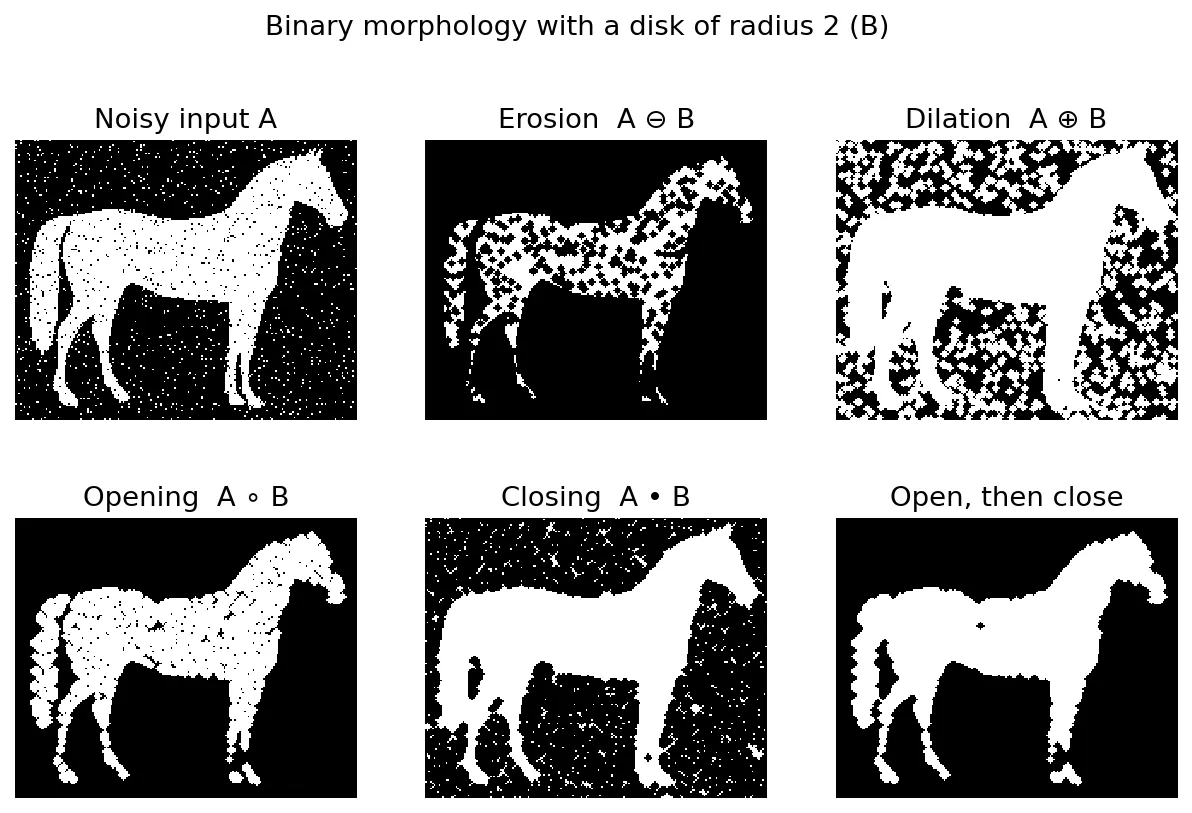
Idempotence is the property that separates opening and closing from erosion and dilation: repeated erosions keep shrinking, while repeated openings stop. Figure 9.1 shows all four operations on a noisy silhouette. The opening removes the white specks in the background; the closing removes the black specks inside the horse; opening followed by closing removes both, a simple and very common morphological noise filter.

import numpy as np
from skimage import data, morphology

A = ~data.horse()
B = morphology.disk(4)
op = morphology.binary_opening(A, B)
cl = morphology.binary_closing(A, B)
print("opening is anti-extensive:", not (op & ~A).any())
print("closing is extensive:     ", not (A & ~cl).any())
print("opening is idempotent:    ", np.array_equal(morphology.binary_opening(op, B), op))

The hit-or-miss transform

In plain words: the hit-or-miss transform (HMT) is a template matcher for binary patterns. You say which pixels must be foreground and which must be background, and it lights up exactly where both conditions hold.

Use two disjoint SEs: $B_1$, the pixels that must lie in the foreground, and $B_2$, the pixels that must lie in the background. The HMT of $A$ is

$$A \circledast B_{1,2} = \{ z \mid (B_1)_z \subseteq A \ \text{and}\ (B_2)_z \subseteq A^c \} = (A \ominus B_1) \cap (A^c \ominus B_2).$$

Here $B_{1,2}$ denotes the pair $(B_1, B_2)$, $A \ominus B_1$ finds positions where the foreground pattern fits, and $A^c \ominus B_2$ finds positions where the background pattern fits. Pixels in neither $B_1$ nor $B_2$ are don’t-care positions. It is common to draw the pair as one small grid with 1 (must be foreground), 0 (must be background) and blank (don’t care).

Some useful templates:

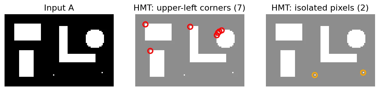
• Isolated point: $B_1$ is the centre pixel; $B_2$ is its 8 neighbours.
• Upper-left corner: $B_1$ is the centre plus its right and lower neighbours; $B_2$ is the upper and left neighbours.
• End point of a one-pixel line: the centre and exactly one neighbour are foreground; the rest are background. You need one template per direction (8 rotations).

Figure 9.2 applies the first two templates. Note that the staircase outline of a digital disk contains several genuine upper-left corners at pixel level: the HMT is literal, not geometric.

import numpy as np
from scipy import ndimage as ndi

A = np.zeros((7, 9), bool)
A[1:5, 1:6] = True                # a rectangle
A[5, 7] = True                    # an isolated pixel
hit  = np.array([[0, 0, 0], [0, 1, 1], [0, 1, 0]], bool)   # must be foreground
miss = np.array([[0, 1, 0], [1, 0, 0], [0, 0, 0]], bool)   # must be background
corners = ndi.binary_hit_or_miss(A, structure1=hit, structure2=miss)
print(np.argwhere(corners))       # [[1 1]]: the upper-left corner only

The HMT is the building block of thinning, thickening and the convex hull algorithm below.

Some basic morphological algorithms

In plain words: with erosion, dilation and the HMT you can build many practical tools. Most of them are short loops that repeat one operation until nothing changes.

Boundary extraction

The inner boundary of a set is what erosion removes:

$$\beta(A) = A - (A \ominus B),$$

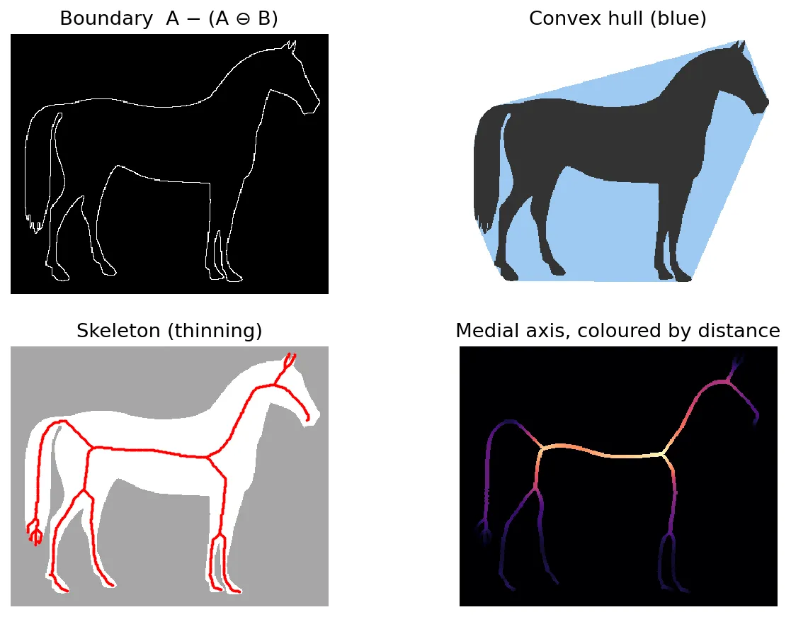
where $B$ is a $3 \times 3$ square (giving an 8-connected boundary) or a cross (giving a thicker, 4-connected one). Using a larger $B$ gives a thicker boundary. The first panel of Figure 9.3 shows $\beta(A)$ for the horse.

Hole filling

A hole is a background region completely surrounded by foreground. Given one seed pixel inside a hole, grow the seed by repeated dilation but clip it to the background at every step:

$$X_k = (X_{k-1} \oplus B) \cap A^c, \qquad k = 1, 2, 3, \ldots$$

Here $X_0$ contains only the seed, $B$ is the 4-connected cross, and the intersection with $A^c$ stops the growth at the hole’s wall. Stop when $X_k = X_{k-1}$; then $X_k \cup A$ is the filled shape. This “dilate, then clip” pattern is called conditional dilation, and it reappears below as geodesic dilation. Using the cross (not the square) as $B$ matters: with an 8-connected foreground wall, the 4-connected background fill cannot leak diagonally through the wall.

import numpy as np
from scipy import ndimage as ndi

def fill_hole(A, seed):
    """Grow X from a seed inside one hole: X_k = dilate(X_{k-1}) AND not A."""
    B = np.array([[0, 1, 0], [1, 1, 1], [0, 1, 0]], bool)   # 4-connected cross
    X = np.zeros_like(A); X[seed] = True
    while True:
        X_next = ndi.binary_dilation(X, structure=B) & ~A
        if np.array_equal(X_next, X):
            return A | X
        X = X_next

yy, xx = np.mgrid[-12:13, -12:13]
ring = (np.hypot(yy, xx) <= 10) & (np.hypot(yy, xx) > 6)   # boolean ring
print(ring.sum(), fill_hole(ring, (12, 12)).sum())        # 204 -> 317

Extraction of connected components

Swap the roles: to extract the connected component of $A$ that contains a seed pixel, grow the seed by dilation but clip it to the foreground:

$$X_k = (X_{k-1} \oplus B) \cap A.$$

With $B$ a $3 \times 3$ square the result is the seed’s 8-connected component; with a cross it is the 4-connected component. Repeating this for every unlabelled seed labels all components. Real libraries use faster one- or two-pass labelling algorithms, but the result is the same: scipy.ndimage.label(A, structure=np.ones((3, 3))) returns a label image and the number of components.

Convex hull

A set is convex if the straight segment between any two of its points stays inside it. The convex hull $C(A)$ is the smallest convex set containing $A$. A purely morphological approximation uses four HMT templates $B^i$, $i = 1, \ldots, 4$, each one detecting background pixels that have foreground on one side (left, top, right, bottom). Starting from $X_0^i = A$, iterate

$$X_k^i = (X_{k-1}^i \circledast B^i) \cup X_{k-1}^i$$

until convergence, giving $D^i$, and take $C(A) = \bigcup_{i=1}^4 D^i$. Each template keeps adding pixels in one direction until no concavity facing that direction remains. The result is the convex hull with respect to those four directions; it can grow beyond the true Euclidean hull, so implementations often limit growth to the bounding box. In practice skimage.morphology.convex_hull_image computes the polygonal hull of the foreground pixel coordinates and rasterises it, which is faster and closer to the Euclidean hull.

Thinning

Thinning removes boundary pixels selectively, without breaking the shape apart, until only a one-pixel-wide line remains. One thinning step with template $B$ is

$$A \otimes B = A - (A \circledast B),$$

which deletes exactly the pixels matched by the HMT. A full thinning cycles through a sequence of templates $\{B^1, B^2, \ldots, B^n\}$, usually 8 rotations of an “edge pixel” pattern,

$$A \otimes \{B\} = (( \cdots ((A \otimes B^1) \otimes B^2) \cdots ) \otimes B^n),$$

and repeats the whole cycle until no pixel changes. The templates are designed so that deleting a matched pixel never disconnects the shape and never removes the endpoint of a line. Zhang and Suen’s parallel thinning algorithm is a widely used, efficient version of this idea [6]; skimage.morphology.skeletonize uses it by default for 2-D images, and skimage.morphology.thin implements a related parallel thinning.

Thickening

Thickening is the dual of thinning: it adds background pixels matched by a template,

$$A \odot B = A \cup (A \circledast B).$$

Rather than designing separate thickening templates, the usual practical route is to thin the background and complement the result. Carried to convergence, thinning the background leaves a thin network of background lines running midway between objects, so thickening is a classic way to grow objects until they meet without ever merging.

Skeletons

The skeleton $S(A)$ is a thin set of lines running down the middle of a shape. One formal definition uses maximal disks: a point is on the skeleton if it is the centre of a disk that fits inside $A$ and is not contained in any other fitting disk. Such disks touch the boundary in at least two places. The skeleton has a purely morphological formula:

$$S(A) = \bigcup_{k=0}^{K} S_k(A), \qquad S_k(A) = (A \ominus kB) - \big( (A \ominus kB) \circ B \big),$$

where $A \ominus kB$ means $k$ successive erosions of $A$ by $B$ and $K$ is the last $k$ before the erosion becomes empty. Each $S_k(A)$ holds the points that are “ridge” points at erosion depth $k$: they are present after $k$ erosions but would not survive an opening at that depth. The decomposition is invertible:

$$A = \bigcup_{k=0}^{K} \big( S_k(A) \oplus kB \big),$$

so storing each $S_k$ with its index $k$ is a lossless shape code. The catch is that this skeleton is not guaranteed to be connected. Thinning gives connected, one-pixel-wide skeletons, and the medial axis (computed from a distance transform) attaches the radius of the maximal disk to each skeleton point, as in the right panel of Figure 9.3.

Pruning

Skeletons are sensitive to boundary noise: a single bump on the outline sprouts a short spur (parasitic branch), visible at the horse’s tail in Figure 9.3. Pruning removes spurs shorter than some length $L$:

1. Thin the skeleton by removing end points (pixels with exactly one 8-neighbour) $L$ times. Every spur of length at most $L$ disappears, but every genuine branch also loses $L$ pixels at its tip.
2. Find the end points of the shortened skeleton.
3. Grow those end points back by $L$ conditional dilations, constrained to the original skeleton, to restore the main branches to full length.
4. Take the union of the shortened skeleton and the regrown tips.

import numpy as np
from scipy import ndimage as ndi
from skimage import data, morphology

def endpoints(S):
    n = ndi.convolve(S.astype(int), np.ones((3, 3), int), mode="constant") - S
    return S & (n == 1)            # foreground pixels with exactly one neighbour

def prune_tips(S, L):
    """Step 1 of pruning: strip L layers of end points."""
    S = S.copy()
    for _ in range(L):
        S &= ~endpoints(S)
    return S

skel = morphology.skeletonize(~data.horse())
print(skel.sum(), prune_tips(skel, 10).sum())

Morphological reconstruction

In plain words: reconstruction lets you say “keep every object that contains this seed” and get the object back exactly, not a rounded copy of it. It uses two images: a marker, which says where to start, and a mask, which says how far you may grow.

Geodesic dilation and erosion

Let $F$ be the marker and $G$ the mask, with $F \subseteq G$. The geodesic dilation of size 1 of $F$ with respect to $G$ is

$$D_G^{(1)}(F) = (F \oplus B) \cap G,$$

where $B$ is a small SE (usually the $3 \times 3$ square). The marker grows by one step but may not leave the mask. Size $n$ means $n$ repetitions: $D_G^{(n)}(F) = D_G^{(1)}\big(D_G^{(n-1)}(F)\big)$. The word geodesic refers to distances measured along paths that stay inside $G$, like walking inside a building rather than through its walls.

The dual geodesic erosion of size 1 is

$$E_G^{(1)}(F) = (F \ominus B) \cup G,$$

with $F \supseteq G$: the marker shrinks, but never below the mask.

Reconstruction by dilation and by erosion

Iterate geodesic dilation until nothing changes. The result is the reconstruction by dilation of mask $G$ from marker $F$:

$$R_G^D(F) = D_G^{(k)}(F) \quad \text{with } k \text{ such that } D_G^{(k)}(F) = D_G^{(k+1)}(F).$$

In binary images, $R_G^D(F)$ is exactly the union of the connected components of $G$ that contain at least one marker pixel. Likewise, the reconstruction by erosion $R_G^E(F)$ iterates geodesic erosion to stability. Vincent’s paper gives the standard efficient algorithms (queue-based, visiting each pixel a bounded number of times rather than iterating full-image passes) and many applications [7]; skimage.morphology.reconstruction follows that approach.

Opening by reconstruction

An ordinary opening removes small objects but also rounds the corners and erases the thin parts of the large ones. Opening by reconstruction avoids that:

$$O_R^{(n)}(F) = R_F^D\big(F \ominus nB\big),$$

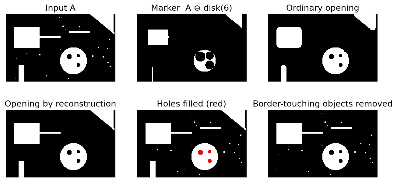
where $F$ is the input image, $F \ominus nB$ is $n$ erosions by $B$ (the marker), and the input itself is the mask. Erosion decides which objects survive (those that contain at least one placement of the SE); reconstruction restores each survivor to its original shape. Compare the “ordinary opening” and “opening by reconstruction” panels of Figure 9.4: the thin arm on the square and the sharp corners return intact. Closing by reconstruction is the dual, built from dilation and reconstruction by erosion.

Automatic hole filling

Reconstruction also fills all holes at once without seeds. Holes are background regions that cannot be reached from the image frame. So build a marker that is the complement of the image on the frame and zero elsewhere,

$$F(x, y) = \begin{cases} 1 - I(x, y) & \text{if } (x, y) \text{ is on the image border,} \\ 0 & \text{otherwise,} \end{cases}$$

reconstruct the background from it, and complement:

$$H = \big[ R_{I^c}^D(F) \big]^c .$$

$R_{I^c}^D(F)$ is the background reachable from the border; everything else, $H$, is the foreground plus its holes.

Border clearing

Objects that touch the image border are often incomplete and should be excluded from measurements. Using the image itself on the border as the marker,

$$F(x, y) = \begin{cases} I(x, y) & \text{if } (x, y) \text{ is on the border,} \\ 0 & \text{otherwise,} \end{cases} \qquad X = I - R_I^D(F),$$

the reconstruction recovers every object that touches the border, and subtracting it leaves only interior objects.

import numpy as np
from skimage import morphology, segmentation

def open_by_reconstruction(A, footprint):
    marker = morphology.binary_erosion(A, footprint)
    return morphology.reconstruction(marker.astype(np.uint8), A.astype(np.uint8),
                                     method="dilation").astype(bool)

def fill_holes_auto(A):
    """Background reachable from the image frame is background; the rest is hole."""
    Ac = ~A
    marker = np.zeros_like(Ac)
    marker[0, :], marker[-1, :] = Ac[0, :], Ac[-1, :]
    marker[:, 0], marker[:, -1] = Ac[:, 0], Ac[:, -1]
    reached = morphology.reconstruction(marker.astype(np.uint8), Ac.astype(np.uint8),
                                        method="dilation").astype(bool)
    return ~reached

# Library shortcuts: scipy.ndimage.binary_fill_holes(A), segmentation.clear_border(A)

Summary of binary operations

The table collects the binary operations of this chapter. Throughout, $A$ is the input set, $B$ the structuring element, $F$ a marker, $G$ a mask, and $B$ is assumed to contain its origin.

Operation	Formula	What it does
Translation	$(B)_z = \{ b + z \}$	Moves the SE’s origin to $z$
Reflection	$\hat{B} = \{ -b \}$	Rotates the SE by 180°
Complement	$A^c$	Swaps foreground and background
Erosion	$A \ominus B$	Keeps positions where $B$ fits; shrinks, removes thin parts
Dilation	$A \oplus B$	Keeps positions where $\hat{B}$ touches $A$; grows, bridges gaps
Opening	$(A \ominus B) \oplus B$	Removes specks, thin necks, sharp corners; idempotent
Closing	$(A \oplus B) \ominus B$	Fills small holes and narrow gaps; idempotent
Hit-or-miss	$(A \ominus B_1) \cap (A^c \ominus B_2)$	Finds an exact foreground/background pattern
Boundary	$A - (A \ominus B)$	One-pixel inner outline
Hole filling	$X_k = (X_{k-1} \oplus B) \cap A^c$	Fills the hole that contains the seed
Connected component	$X_k = (X_{k-1} \oplus B) \cap A$	Extracts the component that contains the seed
Convex hull	union of iterated HMTs	Fills concavities
Thinning	$A - (A \circledast B)$, over a template sequence	Peels pixels to a 1-pixel skeleton, keeps connectivity
Thickening	$A \cup (A \circledast B)$	Dual of thinning
Skeleton	$\bigcup_k (A \ominus kB) - (A \ominus kB) \circ B$	Medial lines; invertible with the index $k$
Pruning	end-point removal, then conditional regrowth	Removes short spurs
Geodesic dilation	$(F \oplus B) \cap G$	One step of growth inside a mask
Geodesic erosion	$(F \ominus B) \cup G$	One step of shrinking above a mask
Reconstruction by dilation	$D_G^{(k)}(F)$ at stability	Components of $G$ hit by $F$
Opening by reconstruction	$R_F^D(F \ominus nB)$	Removes small objects, keeps others exact
Hole filling (auto)	$[R_{I^c}^D(F)]^c$	Fills all holes, no seeds
Border clearing	$I - R_I^D(F)$	Removes border-touching objects

Grayscale morphology

In plain words: for gray images, “fits inside” becomes “local minimum” and “touches” becomes “local maximum”. Picture the image as a landscape where brightness is height. Erosion lowers each pixel to the lowest ground under the stencil; dilation raises it to the highest.

Grayscale erosion and dilation

With a flat SE $b$ (a set of offsets, all of height zero), grayscale erosion and dilation of an image $f$ are

$$[f \ominus b](x, y) = \min_{(s, t) \in b} f(x + s,\ y + t), \qquad [f \oplus b](x, y) = \max_{(s, t) \in b} f(x - s,\ y - t),$$

where $(s, t)$ runs over the SE’s offsets. The minus sign in dilation is the reflection again. On a binary image these reduce exactly to the set definitions. Erosion darkens the image, shrinks bright features and widens dark ones; dilation does the opposite.

A nonflat SE $b_N$ also has heights $b_N(s, t)$:

$$[f \ominus b_N](x, y) = \min_{(s, t) \in b_N} \big\{ f(x + s,\ y + t) - b_N(s, t) \big\}, \qquad [f \oplus b_N](x, y) = \max_{(s, t) \in b_N} \big\{ f(x - s,\ y - t) + b_N(s, t) \big\}.$$

Nonflat SEs are rarely used in practice: the result depends on the image’s intensity scale, and erosion can go below the image’s minimum. Duality carries over with the gray complement $f^c = -f$ (or $L - 1 - f$ for an $L$-level image): $(f \ominus b)^c = f^c \oplus \hat{b}$.

Opening and closing

The definitions are unchanged: $f \circ b = (f \ominus b) \oplus b$ and $f \bullet b = (f \oplus b) \ominus b$. The geometric picture is a ball pushed up from beneath the intensity surface: the opening is the highest surface the ball can reach while staying below $f$. Bright peaks narrower than the ball are cut down; everything wider is left alone. Closing pushes the ball down from above: dark valleys narrower than the ball are filled. The properties (anti-extensive/extensive, increasing, idempotent) carry over with $\le$ in place of $\subseteq$.

Morphological smoothing

Because opening suppresses small bright details and closing suppresses small dark details, the sequence opening followed by closing with the same SE removes both kinds of small structure, while keeping sharp edges of larger regions. This is the grayscale version of the noise filter in Figure 9.1. A related scheme, alternating sequential filtering, applies opening–closing pairs with SEs of increasing size, which avoids the artefacts of using one large SE at once.

Morphological gradient

Dilation minus erosion gives a measure of local contrast:

$$g = (f \oplus b) - (f \ominus b).$$

Inside uniform regions the max and min are nearly equal, so $g \approx 0$; across an edge they differ by the edge height. Unlike a Sobel derivative, $g$ is non-negative and direction-independent (for a symmetric $b$). Using only one side gives the internal gradient $f - (f \ominus b)$ or the external gradient $(f \oplus b) - f$, which place the edge response just inside or just outside the brighter region.

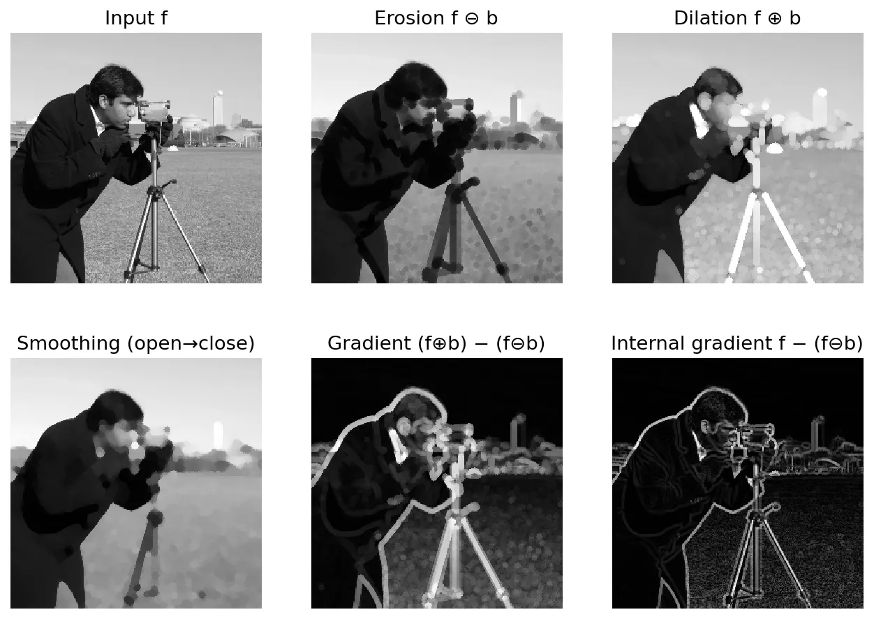
from skimage import data, morphology, util

f = util.img_as_float(data.camera())
b = morphology.disk(3)                       # flat structuring element
ero  = morphology.erosion(f, b)              # local minimum
dil  = morphology.dilation(f, b)             # local maximum
grad = dil - ero                             # morphological gradient (>= 0)
smooth = morphology.closing(morphology.opening(f, b), b)

Top-hat and bottom-hat transforms

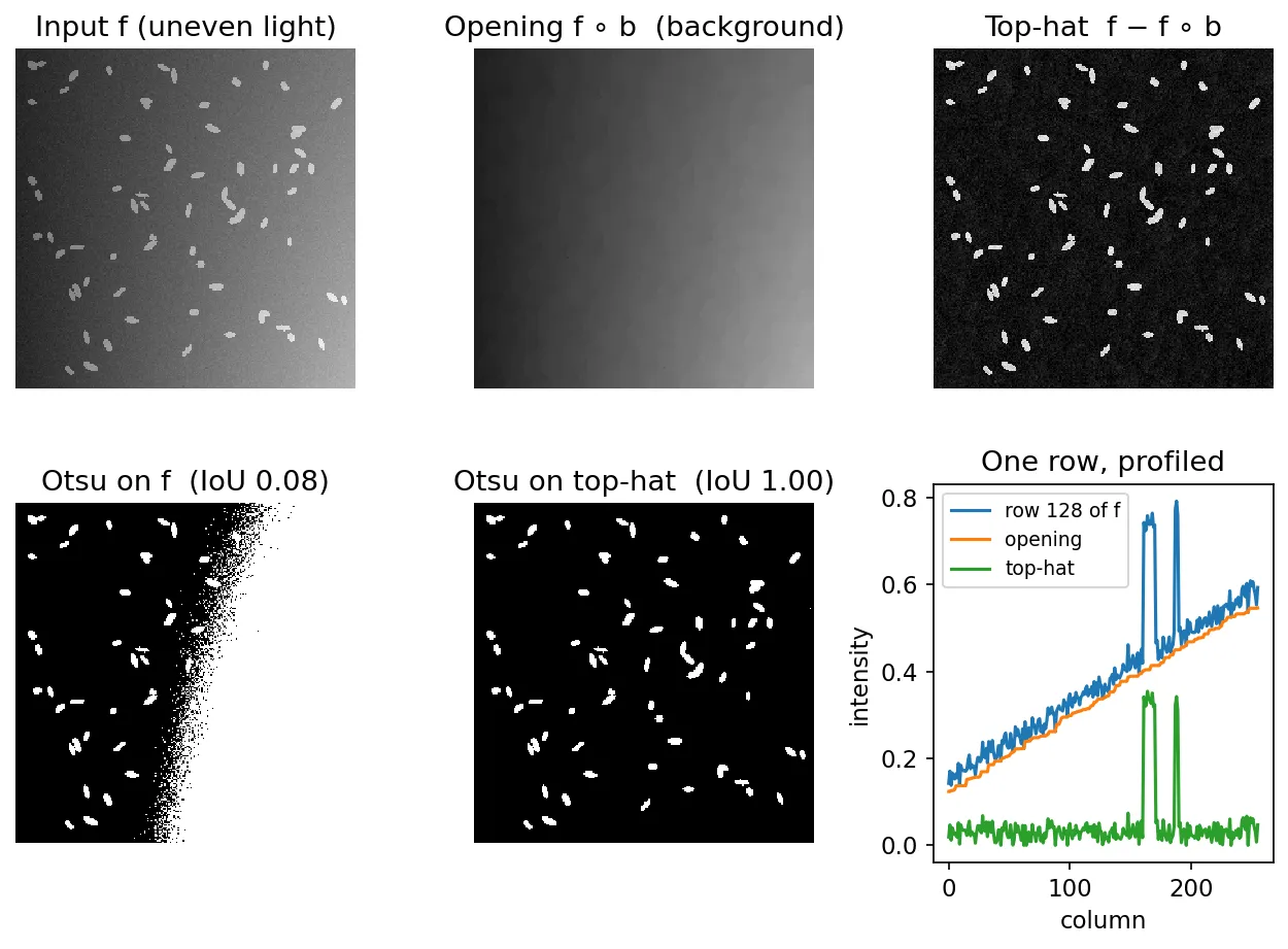
Opening with an SE larger than the bright objects removes those objects but keeps the slowly varying background. Subtracting the opening from the image therefore leaves only the objects. This is the top-hat (or white top-hat) transform:

$$T_{\text{hat}}(f) = f - (f \circ b).$$

Its dual, the bottom-hat (or black top-hat) transform, extracts dark objects on a lighter background:

$$B_{\text{hat}}(f) = (f \bullet b) - f.$$

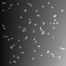
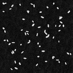
Both are non-negative. The main use is correcting uneven illumination before thresholding. In Figure 9.6, a synthetic image of grains lit from one side defeats a global Otsu threshold (Chapter 10): the bright side of the background is brighter than the grains on the dark side. After a top-hat with a disk of radius 8 (larger than any grain), the background is flat and a single threshold separates the grains almost perfectly. The SE size is the only parameter: it must be larger than the objects and smaller than the scale over which the background changes.

Drag the slider to compare the input with its top-hat:

InputTop-hat (disk r=8)

from skimage import data, filters, morphology, util

coins = util.img_as_float(data.coins())
th = morphology.white_tophat(coins, morphology.disk(30))   # bright objects
bh = morphology.black_tophat(coins, morphology.disk(30))   # dark objects
mask = th > filters.threshold_otsu(th)

Granulometry

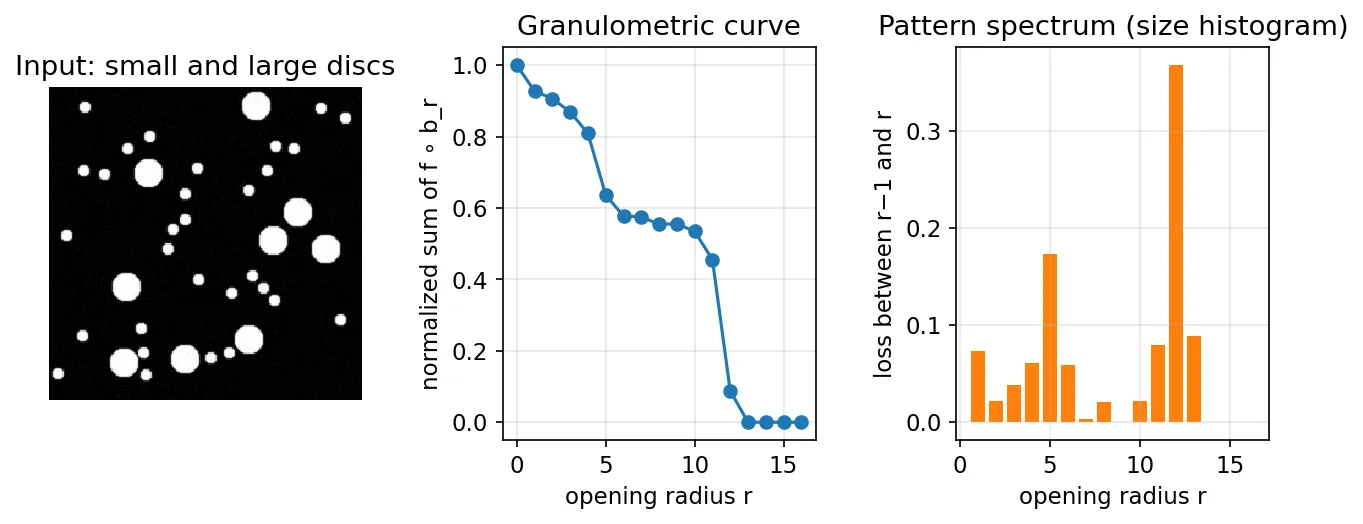
Granulometry measures the size distribution of particles in an image without segmenting them. Open the image with SEs of increasing size $r$; each opening removes the bright particles smaller than $b_r$. Record the total intensity that remains,

$$V(r) = \sum_{x, y} [f \circ b_r](x, y), \qquad r = 0, 1, 2, \ldots,$$

where $b_r$ is a disk of radius $r$ and $b_0$ is a single pixel (so $V(0)$ is the sum of $f$). $V(r)$ never increases, because larger disks fit in fewer places. Its negative discrete derivative,

$$PS(r) = V(r - 1) - V(r),$$

is a size histogram called the pattern spectrum [8]: a large value at $r$ means a lot of image “mass” lives in features of radius about $r$. Figure 9.7 shows a scene with two particle sizes and the two corresponding peaks. The idea of a family of openings indexed by size, with the “sieve” interpretation, goes back to Matheron [2]; Maragos developed the pattern spectrum as a multiscale shape descriptor [8].

import numpy as np
from skimage import morphology

def granulometry(f, radii):
    total = f.sum()
    vol = np.array([morphology.opening(f, morphology.disk(r)).sum() / total
                    for r in radii])
    spectrum = -np.diff(vol)                 # loss from radius r-1 to r
    return vol, spectrum

Textural segmentation

Morphology can also separate regions that differ in the size of their texture elements, for example a field of small blobs next to a field of large blobs. The recipe uses the same size logic as granulometry:

1. Close the image with an SE larger than the gaps between the small blobs (for bright blobs on a dark background, closing fills those dark gaps). The small-blob region turns into a nearly uniform bright patch, while the large blobs, whose gaps are wider than the SE, stay separate.
2. Open the result with an SE larger than the large blobs but smaller than the merged patch. This erases the isolated large blobs and leaves the merged small-blob patch.
3. Take the morphological gradient (or a threshold) of the result. The boundary between the two textures appears as a single strong edge.

The exact SE sizes depend on the blob and gap sizes in your data, which you can measure with a granulometry first.

Grayscale reconstruction

All reconstruction definitions carry over, with $\cap$ replaced by the point-wise minimum $\wedge$ and $\cup$ by the maximum $\vee$. Geodesic dilation of a marker image $f$ under a mask image $g$ (with $f \le g$) is

$$D_g^{(1)}(f) = (f \oplus b) \wedge g,$$

and reconstruction by dilation iterates this to stability. Grayscale reconstruction powers several useful filters [7]:

• Opening by reconstruction, $R_f^D(f \ominus nb)$: removes bright details smaller than the SE but restores the exact shape of everything else. A top-hat by reconstruction, $f - R_f^D(f \ominus nb)$, is cleaner than the ordinary top-hat because the background estimate does not have rounded “shoulders”.
• Regional maxima and the h-dome transform: reconstruct $f$ from the marker $f - h$. The reconstruction flattens every peak of height at most $h$; subtracting it from $f$ keeps only the “domes” (peaks), each at most $h$ tall. Thresholding the domes detects bright blobs regardless of the local background level.

from skimage import data, morphology, util
import numpy as np

f = util.img_as_float(data.camera())
h = 0.1
background = morphology.reconstruction(np.clip(f - h, 0, None), f, method="dilation")
domes = f - background                     # bright peaks, each at most h tall

Modern view

Morphology is old, but it is far from finished. Five lines of work are worth knowing.

Foundations and tutorials. Matheron’s work on random sets [2] and Serra’s Image Analysis and Mathematical Morphology [3] set up the algebra: erosion and dilation as Minkowski operations, openings as “sieves”, and the lattice-theoretic view that later extended everything from sets to gray-level functions. Haralick, Sternberg and Zhuang’s 1987 tutorial [4] is still one of the clearest introductions to binary and grayscale morphology for engineers; it defines the operators, proves their basic properties, and connects them to practical algorithms. Soille’s Morphological Image Analysis [5] is the practitioner’s reference: it covers geodesic transforms, reconstruction, watersheds, granulometries, and efficient implementations, and it is the place to look when a library’s documentation is too terse.

Reconstruction and efficient algorithms. Vincent’s 1993 paper [7] made reconstruction practical. Its main takeaway is that the naive “iterate until stable” loop can be replaced by queue-based algorithms whose cost grows roughly linearly with the image size, which turned reconstruction into an everyday tool for hole filling, regional extrema, and h-domes.

Connected operators and component trees. A filter is connected if it can only remove or merge flat zones (connected regions of constant value) and never creates new contours. Openings by reconstruction are the simplest example. Salembier and Wilkinson’s review [10] explains the family: area openings, attribute filters, levelings, and tree-based filtering. Breen and Jones introduced attribute openings and thinnings [9], which keep or remove a connected component based on an attribute (area, elongation, moment of inertia) rather than whether an SE fits. Efficient implementations represent an image as a max-tree or min-tree (a tree of the connected components of all threshold sets) and filter by pruning the tree. Carlinet and Géraud compare many max-tree construction algorithms in a single framework and give a decision tree for choosing one [11]. scikit-image exposes these as area_opening, area_closing, diameter_opening and max_tree.

Size distributions. Maragos’s pattern spectrum [8] formalised granulometry as a multiscale shape descriptor; it is still used for texture and particle-size analysis, and attribute-based granulometries [9] extend it to shape attributes other than size.

Morphology meets deep learning. Deep learning has changed morphology in two directions.

Morphology inside networks. Max pooling is already a flat grayscale dilation followed by subsampling, so the connection is natural. Several groups have built layers whose structuring elements are learned by gradient descent. Mondal et al. study networks built from learnable dilation and erosion neurons and show that two blocks of dilations and erosions, each followed by a linear combination, can approximate any continuous function [13]. Nogueira et al. propose DeepMorphNet, which replaces convolutions with learnable morphological operations and compares the features it learns with standard convolutional networks [14]. A practical difficulty is that min and max have sparse gradients. Kirszenberg et al. [16] and Hermary et al. [15] build smooth morphological layers from differentiable approximations of max and min (generalised means and soft-max functions whose sharpness is set by a learnable parameter), improving on earlier p-convolution layers, and study when such layers actually recover erosions and dilations. These remain research tools: morphological layers are not a standard component of mainstream vision backbones.

Morphology around networks. In segmentation, morphology is used constantly as post-processing of predicted masks: opening to remove false-positive specks, closing or hole filling to repair fragmented objects, remove_small_objects, border clearing, and skeletons for measuring tubular structures. It also appears inside loss functions. clDice [17] computes a differentiable “soft skeleton” by iterating min- and max-pooling (soft erosion and dilation), and uses overlap between the predicted and true skeletons as a loss that encourages topologically correct segmentation of vessels, roads and neurons.

What has not changed: for cleaning, measuring and correcting binary or grayscale images, the classical operators of this chapter are still the fastest, most predictable tools, and they come with guarantees (idempotence, connectivity, exact shape preservation) that learned filters do not offer.

Key takeaways

• Morphology works with shape, not frequency. It uses only min, max, union and intersection, controlled by a structuring element whose size and shape encode the question you ask.
• Erosion keeps positions where the SE fits; dilation keeps positions where the reflected SE touches. They are duals: eroding the foreground equals dilating the background.
• Opening (erode then dilate) removes small bright parts; closing (dilate then erode) fills small dark gaps. Both are idempotent filters, and opening followed by closing is a robust noise cleaner.
• The hit-or-miss transform matches an exact foreground/background pattern and underlies thinning, thickening, and convex hulls.
• Reconstruction (marker plus mask, grow until stable) keeps whole objects exactly: opening by reconstruction, automatic hole filling and border clearing all follow from it.
• In grayscale, erosion and dilation are local min and max. The gradient, top-hat and bottom-hat give edges, background correction, and small-object extraction; granulometry gives size distributions without segmentation.
• Today morphology lives on as post-processing for neural-network masks, as differentiable building blocks in losses such as clDice, and as a research topic in learnable morphological layers.

Exercises

1. A binary image contains a rectangle 40 pixels wide and 10 pixels tall. Describe its erosion and its opening by (a) a $5 \times 5$ square, (b) a horizontal line 15 pixels long, (c) a vertical line 15 pixels long. Which SE removes the rectangle entirely, and why?

Hint

Erosion keeps the positions of the SE’s origin where the whole SE fits. The $5 \times 5$ square fits at a $36 \times 6$ block of positions, and the opening restores the full rectangle, because the rectangle is a union of fitting squares. The horizontal line also fits, so its opening is again the full rectangle. The vertical line is taller than the rectangle and never fits: both its erosion and its opening are empty.

2. Show that dilation is commutative and associative for sets: $A \oplus B = B \oplus A$ and $(A \oplus B) \oplus C = A \oplus (B \oplus C)$. Use the second identity to explain why dilating twice with a $3 \times 3$ square equals dilating once with a $5 \times 5$ square. Is the same true for erosion?

Hint

Write dilation as the Minkowski sum $\{ a + b \mid a \in A, b \in B \}$; both identities follow from the commutativity and associativity of vector addition. A $3 \times 3$ square plus itself is a $5 \times 5$ square. For erosion, use $(A \ominus B) \ominus C = A \ominus (B \oplus C)$, which follows from duality.

3. Design the hit-or-miss template pair $(B_1, B_2)$ that detects the end points of a one-pixel-wide 8-connected line pointing to the right (the line arrives from the left). How many rotated templates do you need to catch all end points? Test your answer with scipy.ndimage.binary_hit_or_miss on skimage.morphology.skeletonize(~skimage.data.horse()).

Hint

Centre in $B_1$ plus the left neighbour in $B_1$; the other seven neighbours in $B_2$. A line can also arrive diagonally, so you need 8 templates (4 axis directions and 4 diagonals). Compare your total count with the count from a neighbour-counting function like endpoints() in the pruning snippet.

4. Your segmentation network outputs masks of cells. Many masks have small holes, a few single-pixel false positives, and some cells are cut by the image border. Write a five-line post-processing pipeline in scikit-image and justify the order of the steps.

Hint

One reasonable order: remove_small_objects (or a small opening) first, so that specks do not get filled or merged; then binary_fill_holes; then a small closing if contours are ragged; then clear_border; finally label to count. Discuss what would go wrong if you closed before removing specks (nearby specks can merge into a “cell”).

5. For a grayscale image $f$ and a flat SE $b$, prove that the top-hat $T(f) = f - (f \circ b)$ is non-negative and that it is idempotent: $T(T(f)) = T(f)$.

Hint

Non-negativity follows from $f \circ b \le f$. For idempotence, show that $T(f) \circ b = 0$. Take any translate $W$ of $b$ and let $y$ be the point of $W$ where $f$ is smallest. Since the opening is at least $\min_W f$ everywhere on $W$ and at most $f$, it equals $f(y)$ at $y$, so $T(f)(y) = 0$. Every translate of $b$ therefore contains a zero of $T(f)$, the erosion of $T(f)$ by $b$ is zero, and so is its opening.

References

1. R. C. Gonzalez and R. E. Woods, Digital Image Processing, 4th ed., Pearson, 2018, Ch. 9. publisher page
2. G. Matheron, Random Sets and Integral Geometry, Wiley, 1975. library record
3. J. Serra, Image Analysis and Mathematical Morphology, Academic Press, 1982. library record
4. R. M. Haralick, S. R. Sternberg, and X. Zhuang, “Image Analysis Using Mathematical Morphology,” IEEE Trans. Pattern Analysis and Machine Intelligence, vol. PAMI-9, pp. 532–550, 1987. doi
5. P. Soille, Morphological Image Analysis, Springer, 2004. doi
6. T. Y. Zhang and C. Y. Suen, “A Fast Parallel Algorithm for Thinning Digital Patterns,” Communications of the ACM, vol. 27, pp. 236–239, 1984. doi
7. L. Vincent, “Morphological Grayscale Reconstruction in Image Analysis: Applications and Efficient Algorithms,” IEEE Trans. Image Processing, vol. 2, pp. 176–201, 1993. doi
8. P. Maragos, “Pattern Spectrum and Multiscale Shape Representation,” IEEE Trans. Pattern Analysis and Machine Intelligence, vol. 11, no. 7, pp. 701–716, 1989. doi
9. E. J. Breen and R. Jones, “Attribute Openings, Thinnings, and Granulometries,” Computer Vision and Image Understanding, vol. 64, no. 3, pp. 377–389, 1996. doi
10. P. Salembier and M. H. F. Wilkinson, “Connected Operators: A Review of Region-Based Morphological Image Processing Techniques,” IEEE Signal Processing Magazine, vol. 26, no. 6, pp. 136–157, 2009. doi
11. E. Carlinet and T. Géraud, “A Comparative Review of Component Tree Computation Algorithms,” IEEE Trans. Image Processing, vol. 23, pp. 3885–3895, 2014. doi
12. S. van der Walt et al., “scikit-image: Image Processing in Python,” PeerJ, 2014. arXiv
13. R. Mondal, S. Santra, S. S. Mukherjee, and B. Chanda, “Morphological Network: How Far Can We Go with Morphological Neurons?,” BMVC, 2022. arXiv
14. K. Nogueira, J. Chanussot, M. Dalla Mura, and J. A. dos Santos, “An Introduction to Deep Morphological Networks,” arXiv:1906.01751, 2019. arXiv
15. R. Hermary, G. Tochon, É. Puybareau, A. Kirszenberg, and J. Angulo, “Learning Grayscale Mathematical Morphology with Smooth Morphological Layers,” Journal of Mathematical Imaging and Vision, vol. 64, pp. 736–753, 2022. doi
16. A. Kirszenberg, G. Tochon, É. Puybareau, and J. Angulo, “Going Beyond p-convolutions to Learn Grayscale Morphological Operators,” arXiv:2102.10038, 2021. arXiv
17. S. Shit et al., “clDice — A Novel Topology-Preserving Loss Function for Tubular Structure Segmentation,” CVPR, 2021. arXiv