Chapter 12 · Feature Extraction

What you’ll learn

• The difference between a feature and a descriptor, and the four invariances most descriptors try to have: translation, rotation, scale and illumination.
• How to turn a segmented boundary into something measurable: chain codes, polygons, signatures and skeletons, and then into numbers such as shape numbers and Fourier descriptors.
• How to describe whole regions by size, shape, topology (Euler number), texture (histogram moments, co-occurrence matrices, spectra) and moment invariants.
• How principal component analysis (PCA) aligns objects and compresses many measurements into a few.
• How the Harris–Stephens corner detector, maximally stable extremal regions (MSER) and SIFT find and describe interest points that can be matched across two photos.
• How surveys of the last two decades judge these handcrafted features, and where learned features (SuperPoint, LoFTR, LightGlue, DINOv2) have replaced them.

The big picture

Segmentation (Chapters 10 and 11) told us where objects are. A program still cannot “look at” a region the way we do. It needs a short list of numbers that says what the region is like, so that it can compare, sort, search and recognize. Producing that list is feature extraction.

This chapter follows the order of Gonzalez and Woods [1]. We start with boundaries, move to regions, then to statistics over many measurements (PCA), and end with features that need no segmentation at all: corners, stable regions and SIFT keypoints. These last ones connect classical image processing to modern computer vision tasks such as panorama stitching, 3D reconstruction and visual localization.

Background: features, descriptors and invariance

Plain version. A feature is something interesting you found in an image (a corner, a blob, a region). A descriptor is the list of numbers you use to describe it. We want descriptors that do not change when things that do not matter change.

Precise version. Following [1], we separate two steps:

• Feature detection finds where a feature is: a boundary, a region, a point with its scale and orientation.
• Feature description assigns a vector $\mathbf{d} \in \mathbb{R}^n$ to each detected feature.

A descriptor $\mathbf{d}(\cdot)$ is invariant to a family of transformations $\mathcal{T}$ if

$$\mathbf{d}(T(f)) = \mathbf{d}(f) \quad \text{for all } T \in \mathcal{T},$$

where $f$ is the image (or region) and $T$ a transformation applied to it. It is covariant if the detected quantity changes with the transformation in a predictable way (for example, a keypoint’s position moves with the object, and its detected scale doubles when the object doubles). Detectors should be covariant; descriptors should be invariant.

The transformations we care about most are:

Change	What it does to the image	Typical cure
Translation	shifts coordinates	subtract a centroid, or use differences
Rotation	rotates coordinates	use a canonical orientation, magnitudes, or rotation-free quantities
Scale	multiplies coordinates	normalize by size, or search over scale
Illumination	changes intensities, roughly $f \mapsto af + b$	use gradients (remove $b$) and normalize (remove $a$)

There is always a trade-off between invariance and discriminative power. A descriptor invariant to everything describes nothing: a “6” rotated by 180° is a “9”. Choosing features is choosing which differences matter for your task.

Boundary preprocessing

Plain version. Before we can measure a boundary, we must list its pixels in order and, often, simplify it so that noise and pixel staircases do not dominate.

Boundary following

A segmented region is a set of pixels. Most boundary descriptors need the boundary as an ordered, closed sequence of points. The standard Moore boundary-following procedure [1] starts at the uppermost-leftmost foreground pixel $b_0$ and its background neighbor $c_0$ to the west. It then walks clockwise around the 8-neighborhood of the current boundary pixel, starting at $c$, until it hits a foreground pixel. That pixel becomes the next boundary point, the background pixel just checked before it becomes the new $c$, and the walk repeats until it returns to $b_0$ moving toward the second point. The result is a list $(x_0, y_0), \dots, (x_{K-1}, y_{K-1})$. OpenCV’s cv2.findContours and scikit-image’s measure.find_contours give you this list directly.

Chain codes

A chain code replaces the list of points with a list of directions. Each step from one boundary pixel to the next is one of 4 or 8 directions, coded 0–3 or 0–7 counterclockwise from east [1]. The code is compact (3 bits per step for 8 directions) and already independent of translation.

Two problems remain. The code depends on the start point, and it depends on rotation. The fixes are simple:

• Start point. Treat the code as circular and choose the rotation of the sequence that forms the smallest integer.
• Rotation (by multiples of 45°). Use the first difference: the number of direction changes, counted counterclockwise, between consecutive elements, $d_k = (c_k - c_{k-1}) \bmod 8$, where $c_k$ is the $k$-th code element. Turning the object by 90° adds 2 to every $c_k$ and leaves every $d_k$ unchanged.

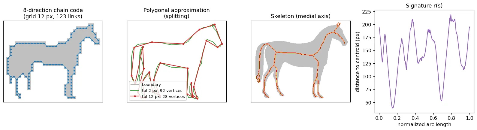
Raw chain codes on the full pixel grid are long and noisy. In practice the boundary is first resampled on a coarser grid, so that each link spans several pixels (Figure 12.1, left).

import numpy as np, cv2
from skimage import data

mask = (data.horse() == 0).astype(np.uint8)          # True inside the horse
cnts, _ = cv2.findContours(mask, cv2.RETR_EXTERNAL, cv2.CHAIN_APPROX_NONE)
pts = max(cnts, key=len)[:, 0, :]                    # (x, y), 8-connected boundary

# Freeman 8-direction code: 0 = east, counted counter-clockwise (y points down)
DIRS = {(1, 0): 0, (1, -1): 1, (0, -1): 2, (-1, -1): 3,
        (-1, 0): 4, (-1, 1): 5, (0, 1): 6, (1, 1): 7}
steps = np.diff(np.vstack([pts, pts[:1]]), axis=0)
code = np.array([DIRS[tuple(s)] for s in steps])

diff = (code - np.roll(code, 1)) % 8                 # first difference: rotation invariant
shifts = [tuple(np.roll(diff, -i)) for i in range(len(diff))]
shape_number = min(shifts)                           # start-point invariant
print(len(code), code[:12], diff[:12])

Slope chain codes

Ordinary chain codes only know eight directions. A slope chain code (SCC) [1] instead places straight segments of equal length along the curve, end to end, and records the change of slope between consecutive segments as a real number, normalized to the interval $(-1, 1]$ (so $\pm 1$ means a full reversal). Because only changes in direction are recorded, the SCC is invariant to translation and rotation; because all segments have the same length, it becomes invariant to scale once the segment length is set relative to the curve length. The sum of the absolute slope changes is a natural measure of how winding (tortuous) a curve is.

Polygonal approximation

A polygon can capture the essence of a boundary with a few vertices.

Minimum-perimeter polygons (MPP). Cover the boundary with a strip of square cells (a “cellular complex”). Its inner and outer walls form two closed fences. Now imagine a rubber band placed between the fences and allowed to shrink: it settles into the shortest closed path that stays inside the strip. That path is the MPP [1]. Its vertices are always at convex corners of the inner wall or concave corners of the outer wall, which leads to an efficient algorithm. The cell size controls the detail: big cells give a coarse polygon.

Merging. Walk along the boundary and keep adding points to the current segment while the least-squares line-fit error stays below a threshold $T$. When the error exceeds $T$, start a new segment. This is simple, but vertices may not land at true corners.

Splitting. Join the two most distant boundary points with a chord. Find the boundary point farthest from that chord; if its distance exceeds $T$, make it a vertex and split the problem in two. Repeat recursively. Splitting tends to place vertices at real inflection points. skimage.measure.approximate_polygon implements this recursive splitting idea; Figure 12.1 (second panel) shows two tolerances.

Signatures

A signature reduces a 2-D boundary to a 1-D function. The simplest is the distance from the centroid to the boundary as a function of angle, $r(\theta)$, or of normalized arc length, $r(s)$ [1]. A circle gives a constant; a square gives four identical bumps. Signatures are translation invariant by construction. Rotation becomes a circular shift of the function, and scale becomes a multiplication, so we normalize by choosing a canonical start (for example the farthest point) and dividing by the maximum or by the standard deviation. $r(\theta)$ is a function only for star-shaped regions; for shapes like the horse in Figure 12.1, a ray from the centroid can cross the boundary more than once, which is why $r(s)$ is used there.

Skeletons and the medial axis

Plain version. Light a fire on the entire edge of a grass field at the same moment. The places where fire fronts from different sides meet form the skeleton.

Precise version. The medial axis of a region $R$ with border $B$ is the set of points in $R$ that have more than one closest point on $B$ [1]. Each medial-axis point, together with its distance to the border, defines a maximal inscribed disk; the union of these disks reconstructs $R$ exactly (the medial axis transform). Computing it directly is expensive, so practical skeletons are found by thinning: repeatedly deleting border pixels that are not endpoints and whose removal does not break connectivity, until nothing more can be removed. Skeletons are very sensitive to small bumps on the boundary, so smoothing or pruning short branches is usually needed.

Boundary feature descriptors

Plain version. Once a boundary is an ordered list, we can measure it: how long it is, how wide, how bent, and how it looks when written as a sum of waves.

Basic descriptors

• Length. The number of pixels on the boundary is a rough estimate. With an 8-connected chain code, count horizontal and vertical steps as 1 and diagonal steps as $\sqrt{2}$.
• Diameter. $\operatorname{Diam}(B) = \max_{i,j} D(p_i, p_j)$, where $p_i, p_j$ are boundary points and $D$ is a distance (usually Euclidean). The segment joining the two maximizing points is the major axis; the minor axis is perpendicular to it, with length chosen so that a box with these two sides encloses the boundary. That box is the basic rectangle.
• Eccentricity. The ratio of major-axis length to minor-axis length. (Region-based eccentricity, below, uses second moments instead.)
• Curvature. The rate of change of slope along the boundary. On a digital boundary it is noisy, so we usually compute the slope difference between line segments fitted on either side of a point. Where curvature changes sign, the boundary has an inflection; positive curvature (in the walking direction) marks a convex part, negative a concave part.

Shape numbers

The shape number of a boundary is the first difference of its 4-direction chain code, circularly shifted to form the smallest integer [1]. Its length is the order $n$ of the shape. For a closed boundary on a 4-connected grid, $n$ is always even, and only a finite number of shapes exist for each order. To compare two shapes fairly, we first fix the orientation: align the grid with the shape’s basic rectangle (or major axis), pick the grid size that gives the desired order, compute the chain code there, then the shape number. Two shapes can then be compared by their degree of similarity, the largest order for which their shape numbers still agree.

Fourier descriptors

Plain version. Walk around the boundary and write each point as a complex number. The sequence repeats every lap, so we can decompose it into waves. The first few, slow waves give the rough outline; fast waves add the details.

Precise version. Let the boundary be $K$ points $(x_k, y_k)$, $k = 0, \dots, K-1$, and write each as

$$s(k) = x(k) + j\,y(k).$$

The discrete Fourier transform of $s(k)$ gives the Fourier descriptors

$$a(u) = \sum_{k=0}^{K-1} s(k)\, e^{-j 2\pi u k / K}, \qquad u = 0, 1, \dots, K-1,$$

and the inverse rebuilds the boundary. If we keep only $P$ of the coefficients (the lowest frequencies, both positive and negative) and set the rest to zero, we get an approximation $\hat{s}(k)$ that is smooth and keeps the overall shape (Figure 12.2). This is why a handful of Fourier descriptors can represent a shape compactly.

The descriptors react to basic geometric changes in simple ways [1]:

Change to the boundary	Effect on $a(u)$
Translation by $\Delta_{xy} = \Delta_x + j\Delta_y$	only $a(0)$ changes: $a(0) + K\Delta_{xy}$
Rotation by $\theta$	every coefficient is multiplied by $e^{j\theta}$
Scaling by $\alpha$	every coefficient is multiplied by $\alpha$
Start point moved by $k_0$	$a(u)$ is multiplied by $e^{-j 2\pi k_0 u / K}$

So we can build an invariant descriptor: drop $a(0)$ (translation), divide by $|a(1)|$ (scale), and keep only magnitudes $|a(u)|$ (rotation and start point). The cost of keeping only magnitudes is losing phase, which carries part of the shape information.

import numpy as np
from skimage import data, measure

mask = data.horse() == 0
c = max(measure.find_contours(mask.astype(float), 0.5), key=len)
z = c[:, 1] + 1j * c[:, 0]                       # boundary as complex numbers x + jy

def fourier_descriptor(z, n=16):
    a = np.fft.fft(z)
    a[0] = 0                                     # drop DC   -> translation invariance
    a = a / np.abs(a[1])                         # divide by |a(1)| -> scale invariance
    return np.abs(np.r_[a[1:n + 1], a[-n:]])     # magnitudes -> rotation and start-point invariance

f1 = fourier_descriptor(z)
f2 = fourier_descriptor(0.5 * np.exp(1j * 0.7) * np.roll(z, 300) + (40 + 10j))
print(np.abs(f1 - f2).max())                     # ~1e-16: same descriptor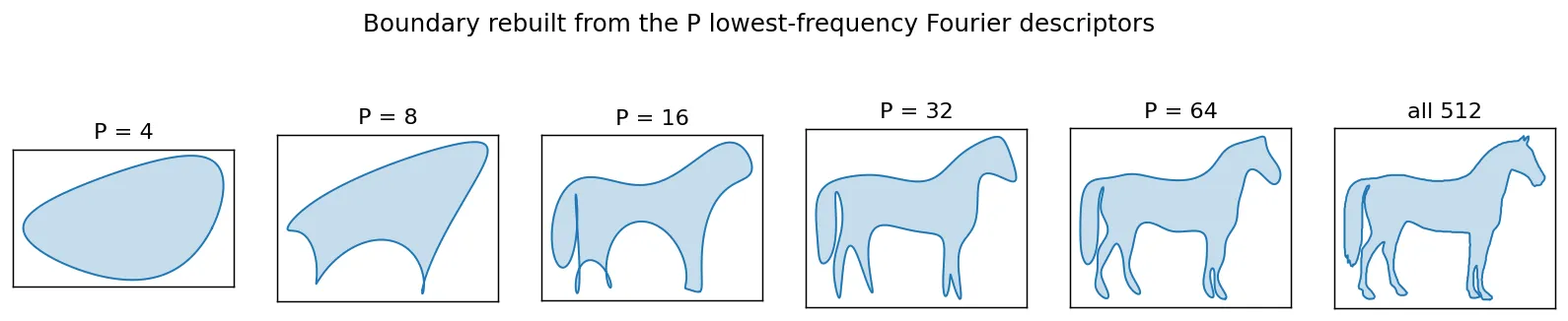

Statistical moments of a boundary

A boundary segment, or a signature, is a 1-D function $g(r)$. Treat its amplitude as a random variable $v$ and form a histogram $p(v_i)$, $i = 0, \dots, A-1$, where $A$ is the number of amplitude bins. Then

$$\mu_n(v) = \sum_{i=0}^{A-1} (v_i - m)^n\, p(v_i), \qquad m = \sum_{i=0}^{A-1} v_i\, p(v_i),$$

where $m$ is the mean amplitude and $\mu_n$ the $n$-th central moment [1]. $\mu_2$ measures spread and $\mu_3$ asymmetry. Alternatively, normalize $g(r)$ to unit area and treat it as a density over $r$; the moments then describe the shape of the curve. Moments are cheap, physically interpretable, and insensitive to rotation (if computed on a rotation-normalized signature).

Region feature descriptors

Plain version. Instead of tracing the edge, we can look at the whole patch: how big it is, how round, how many holes it has, and how its inside looks (smooth, grainy, striped).

Basic descriptors

• Area $A$: the number of pixels in the region.
• Perimeter $P$: the length of its boundary.
• Compactness: $P^2 / A$. It is dimensionless, so it is invariant to scale (and to translation and rotation, up to digitization error). A disk minimizes it.
• Circularity: $R_c = 4\pi A / P^2$. It equals 1 for a disk and decreases for elongated or ragged regions. It is the inverse of compactness, rescaled.
• Effective diameter: $d_e = 2\sqrt{A/\pi}$, the diameter of a disk with the same area.
• Eccentricity (from moments): with $\lambda_1 \ge \lambda_2$ the eigenvalues of the covariance matrix of the pixel coordinates, $e = \sqrt{1 - \lambda_2/\lambda_1}$. It is 0 for a disk and approaches 1 for a line segment. (This is the definition used by scikit-image.)

import numpy as np
from skimage import data, filters, measure, morphology, segmentation

img = data.coins()
bw = img > filters.threshold_otsu(img)
bw = morphology.binary_closing(bw, morphology.disk(2))
bw = segmentation.clear_border(morphology.remove_small_objects(bw, 200))
for r in measure.regionprops(measure.label(bw))[:4]:
    circ = 4 * np.pi * r.area / r.perimeter ** 2  # 1 for a perfect disk
    print(f"area={r.area:5.0f}  circularity={circ:.2f}  "
          f"eccentricity={r.eccentricity:.2f}  euler={r.euler_number}  "
          f"hu1={r.moments_hu[0]:.4f}")

On the coins image, the well-segmented coins have circularity around 0.9 and eccentricity around 0.3–0.4 (digital perimeters are slightly overestimated, so even a perfect digital disk scores a bit below 1).

Topological descriptors

Topology studies properties that survive rubber-sheet deformations: stretching and bending without tearing or gluing. Area and perimeter are not topological; the number of pieces and the number of holes are. The Euler number is

$$E = C - H,$$

where $C$ is the number of connected components and $H$ the number of holes [1]. The letter “A” has $E = 0$ (one component, one hole); “B” has $E = -1$. For regions represented as straight-line networks (polygonal networks), Euler’s formula connects topology to counting:

$$V - Q + F = C - H = E,$$

where $V$ is the number of vertices, $Q$ the number of edges and $F$ the number of faces. Note that $E$ depends on the connectivity convention (4 or 8) used for foreground and background.

Texture

Plain version. Texture is how a surface “feels” to the eye: smooth, coarse, regular. We describe it with statistics of the pixel values and of how pixel values sit next to each other.

Statistical moments of the histogram. Let $z$ be a random variable for intensity, $p(z_i)$ the normalized histogram, $i = 0, \dots, L-1$, and $m = \sum_i z_i p(z_i)$ the mean. Then [1]:

$$\begin{aligned} \mu_n(z) &= \sum_{i=0}^{L-1} (z_i - m)^n\, p(z_i) && \text{(}n\text{-th central moment)}\\ R(z) &= 1 - \frac{1}{1 + \sigma^2(z)} && \text{(relative smoothness; } \sigma^2 = \mu_2\text{)}\\ U(z) &= \sum_{i=0}^{L-1} p^2(z_i) && \text{(uniformity)}\\ e(z) &= -\sum_{i=0}^{L-1} p(z_i) \log_2 p(z_i) && \text{(entropy)} \end{aligned}$$

$R$ is 0 for a constant region and approaches 1 for high variance (normalize $\sigma^2$ to $[0,1]$ first, for example by dividing by $(L-1)^2$). $\mu_3$ measures histogram skew. These measures ignore where pixels are, so a checkerboard and its shuffled version get identical values.

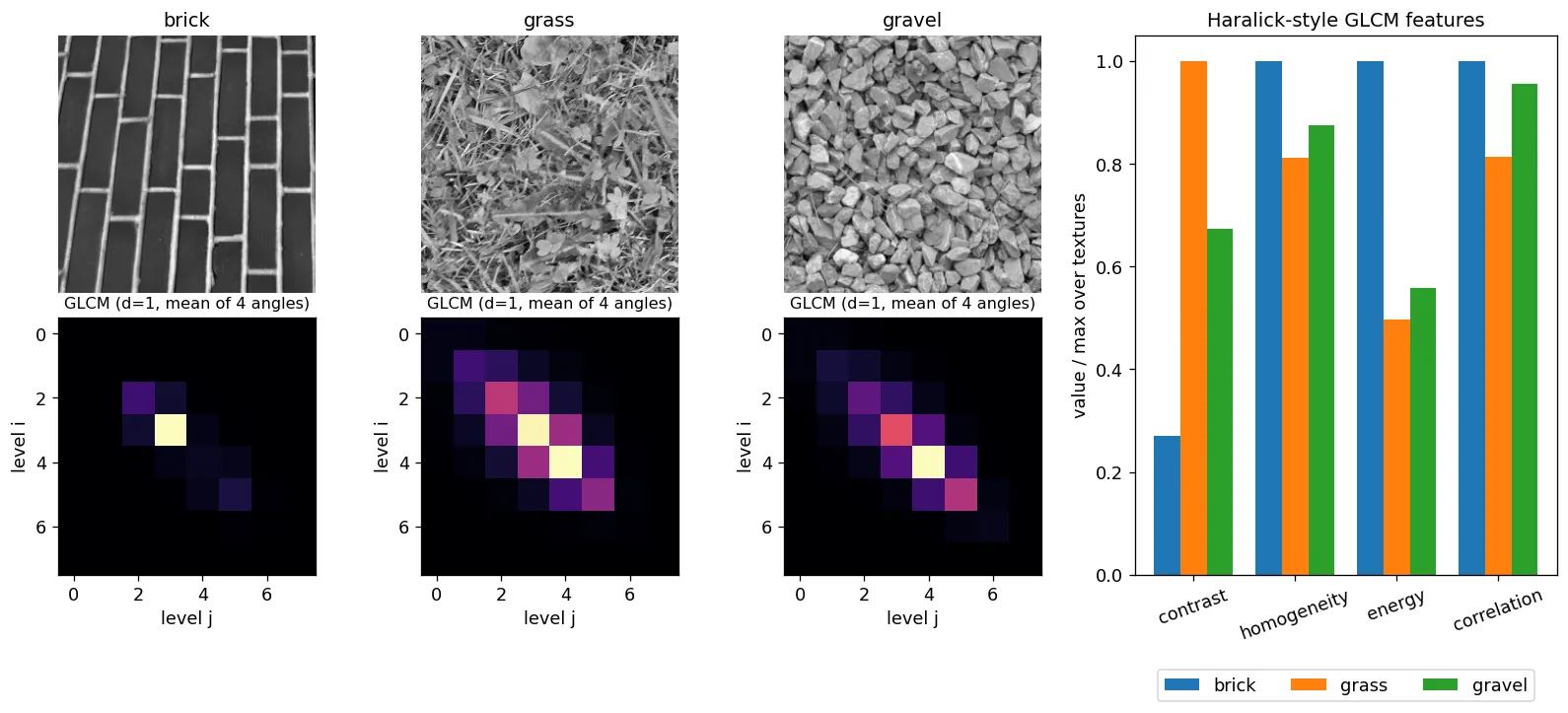
Co-occurrence matrices. To capture spatial arrangement, Haralick, Shanmugam and Dinstein proposed the gray-level co-occurrence matrix (GLCM) [3]. Fix a position operator $Q$, for example “one pixel to the right”. Then $G$ is an $L \times L$ matrix whose element $g_{ij}$ counts how many times a pixel with level $i$ has a pixel with level $j$ in position $Q$. Let $n = \sum_{i,j} g_{ij}$ and

$$p_{ij} = g_{ij} / n,$$

the estimated probability of that pair. Useful descriptors computed from $p_{ij}$ include (with $m_r, m_c$ and $\sigma_r, \sigma_c$ the means and standard deviations of the row and column marginals):

$$\begin{aligned} \text{Contrast} &= \sum_{i,j} (i - j)^2\, p_{ij} \qquad \text{Homogeneity} = \sum_{i,j} \frac{p_{ij}}{1 + |i - j|}\\ \text{Uniformity (energy)} &= \sum_{i,j} p_{ij}^2 \qquad \text{Entropy} = -\sum_{i,j} p_{ij} \log_2 p_{ij}\\ \text{Correlation} &= \sum_{i,j} \frac{(i - m_r)(j - m_c)\, p_{ij}}{\sigma_r \sigma_c} \end{aligned}$$

(scikit-image’s graycoprops reports “energy” as the square root of the uniformity sum.) Mass near the diagonal means neighbors have similar values (smooth texture, high homogeneity, low contrast). Mass spread away from the diagonal means rapid changes (high contrast). In practice we quantize to few levels (8–32), compute $G$ for several angles and distances, and average over angles for approximate rotation invariance.

import numpy as np
from skimage import data
from skimage.feature import graycomatrix, graycoprops

for name in ["brick", "grass", "gravel"]:
    q = (getattr(data, name)()[:256, :256] // 32).astype(np.uint8)   # 8 gray levels
    P = graycomatrix(q, distances=[1], angles=[0, np.pi/4, np.pi/2, 3*np.pi/4],
                     levels=8, symmetric=True, normed=True)
    feats = {p: graycoprops(P, p).mean() for p in ["contrast", "homogeneity", "energy", "correlation"]}
    print(name, {k: round(float(v), 3) for k, v in feats.items()})

brick  {'contrast': 0.269, 'homogeneity': 0.883, 'energy': 0.579, 'correlation': 0.817}
grass  {'contrast': 0.995, 'homogeneity': 0.717, 'energy': 0.288, 'correlation': 0.664}
gravel {'contrast': 0.669, 'homogeneity': 0.772, 'energy': 0.323, 'correlation': 0.78}

The brick wall is dominated by large flat bricks, so its GLCM is concentrated on a few diagonal cells: high energy, low contrast. Grass changes from blade to blade, so its GLCM spreads out: highest contrast, lowest energy. Four numbers already separate the three textures (Figure 12.3).

Spectral texture. Periodic or directional texture produces strong, concentrated peaks in the Fourier spectrum. Write the spectrum in polar coordinates, $S(r, \theta)$, where $r$ is the distance from the origin (frequency) and $\theta$ the direction. Two 1-D functions summarize it [1]:

$$S(r) = \sum_{\theta=0}^{\pi} S_\theta(r), \qquad S(\theta) = \sum_{r=1}^{R_0} S_r(\theta),$$

where $S_\theta(r)$ is the spectrum along the ray at angle $\theta$, $S_r(\theta)$ the spectrum on the half-circle of radius $r$, and $R_0$ the largest radius considered. Peaks in $S(r)$ reveal the period of the pattern (the brick spacing); peaks in $S(\theta)$ reveal its dominant directions. Only half the circle is needed because the spectrum of a real image is symmetric about the origin.

Moment invariants

For a 2-D image (or region indicator) $f(x, y)$ of size $M \times N$, the moment of order $(p + q)$ is

$$m_{pq} = \sum_{x=0}^{M-1} \sum_{y=0}^{N-1} x^p y^q f(x, y),$$

and the central moment is

$$\mu_{pq} = \sum_{x}\sum_{y} (x - \bar{x})^p (y - \bar{y})^q f(x, y), \qquad \bar{x} = \frac{m_{10}}{m_{00}},\ \bar{y} = \frac{m_{01}}{m_{00}},$$

where $(\bar{x}, \bar{y})$ is the centroid. Central moments are translation invariant. Normalized central moments

$$\eta_{pq} = \frac{\mu_{pq}}{\mu_{00}^{\gamma}}, \qquad \gamma = \frac{p + q}{2} + 1,$$

are also scale invariant. Hu [2] derived seven combinations of the second- and third-order $\eta_{pq}$ that are invariant to translation, scale and rotation. The first two are

$$\phi_1 = \eta_{20} + \eta_{02}, \qquad \phi_2 = (\eta_{20} - \eta_{02})^2 + 4\eta_{11}^2.$$

$\phi_1$ is the normalized “moment of inertia” about the centroid: it grows as mass moves away from the center. $\phi_2$ measures elongation. The seventh invariant changes sign under reflection, so it can tell a shape from its mirror image. Because higher-order moments amplify noise, and their values span many orders of magnitude, people usually compare $\operatorname{sign}(\phi_i)\log|\phi_i|$. In scikit-image, regionprops(...).moments_hu returns all seven; in OpenCV, cv2.HuMoments(cv2.moments(mask)).

Principal components as feature descriptors

Plain version. When we measure many things about an object, some measurements tell the same story twice. PCA finds a new set of axes ordered from “most informative” to “least informative”, so we can keep the first few and drop the rest. For a 2-D shape, the first axis is simply the direction in which the shape is longest.

Precise version. Let $\mathbf{x}_1, \dots, \mathbf{x}_K$ be $n$-dimensional vectors: for example the $n$ band values of each pixel in a multispectral image, or the $(x, y)$ coordinates of each pixel of a region. Their mean and covariance are

$$\mathbf{m}_x = \frac{1}{K}\sum_{k=1}^{K} \mathbf{x}_k, \qquad \mathbf{C}_x = \frac{1}{K-1}\sum_{k=1}^{K} (\mathbf{x}_k - \mathbf{m}_x)(\mathbf{x}_k - \mathbf{m}_x)^{\mathsf T}.$$

$\mathbf{C}_x$ is real and symmetric, so it has $n$ orthonormal eigenvectors $\mathbf{e}_i$ with eigenvalues $\lambda_1 \ge \lambda_2 \ge \dots \ge \lambda_n \ge 0$. Stack the eigenvectors as rows of a matrix $\mathbf{A}$. The Hotelling transform (also called the discrete Karhunen–Loève transform, or PCA) is

$$\mathbf{y} = \mathbf{A}(\mathbf{x} - \mathbf{m}_x).$$

The new vectors have zero mean and a diagonal covariance, $\mathbf{C}_y = \mathbf{A}\mathbf{C}_x\mathbf{A}^{\mathsf T} = \operatorname{diag}(\lambda_1, \dots, \lambda_n)$: the components of $\mathbf{y}$ are uncorrelated, and the variance along the $i$-th axis is $\lambda_i$. If we keep only the first $k$ rows, $\mathbf{A}_k$, the reconstruction $\hat{\mathbf{x}} = \mathbf{A}_k^{\mathsf T}\mathbf{y} + \mathbf{m}_x$ has mean squared error

$$e_{\text{ms}} = \sum_{j=k+1}^{n} \lambda_j,$$

the sum of the discarded eigenvalues. No other linear projection onto $k$ dimensions does better in this sense.

Three uses in image processing [1]:

1. Compressing multispectral images. With $n$ registered bands, each pixel is an $n$-vector. Most of the variance usually sits in the first two or three principal-component images, so they can replace all $n$ bands for display or classification.
2. Normalizing object pose. Use the pixel coordinates of a region as the vectors. Then $\mathbf{y} = \mathbf{A}(\mathbf{x} - \mathbf{m}_x)$ moves the centroid to the origin and rotates the region so that its major axis lies along the first coordinate axis (Figure 12.4). Descriptors computed afterwards are translation and rotation invariant; dividing by $\sqrt{\lambda_1}$ adds scale invariance. One caveat: an eigenvector’s sign is arbitrary, so the aligned object may be flipped; a rule such as “the heavier third-moment side points right” resolves it.
3. Eigen-images. Flatten each of many same-size images of one object class into a vector. The leading eigenvectors, reshaped back to images, are “eigen-images” that span most of the variation in the set. Any new image can then be described by its handful of coordinates $\mathbf{y}$, a compact feature vector for recognition.

import numpy as np
from skimage import data, transform

mask = transform.rotate((data.horse() == 0).astype(float), 35, resize=True) > 0.5
X = np.argwhere(mask)[:, ::-1].astype(float)     # (x, y) of every object pixel
m = X.mean(axis=0)
C = np.cov((X - m).T)                            # 2x2 covariance matrix
evals, evecs = np.linalg.eigh(C)                 # ascending eigenvalues
A = evecs[:, ::-1].T                             # rows = eigenvectors, largest first
Y = (X - m) @ A.T                                # Hotelling transform y = A(x - m)
print(np.round(np.cov(Y.T), 3))                  # diagonal: the axes are decorrelated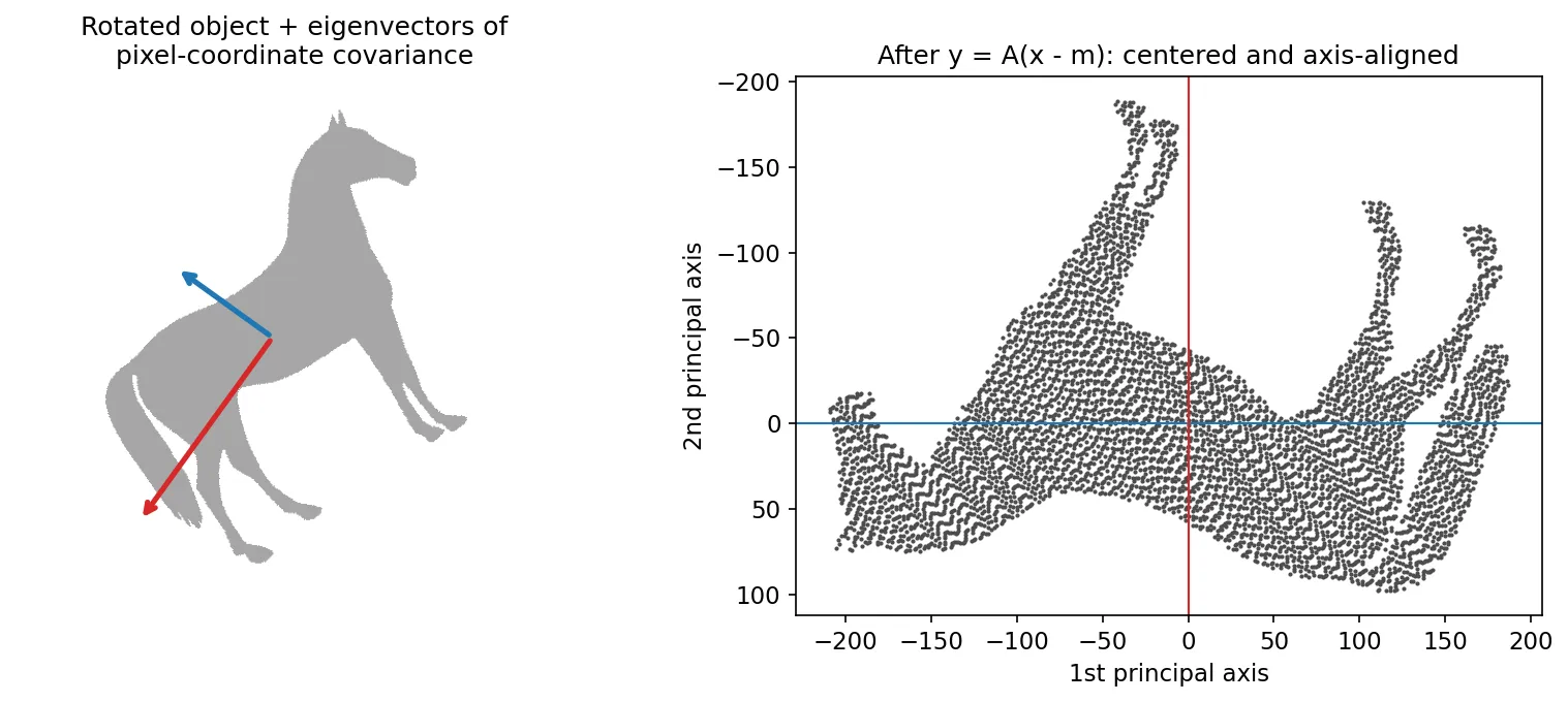

Whole-image features

Plain version. So far we needed a segmented object. Many tasks (stitching panoramas, tracking, 3D reconstruction) instead need landmarks that can be found automatically in any photo and found again in another photo of the same scene. Corners and stable blobs are good landmarks.

The Harris–Stephens corner detector

Plain version. Look at the image through a tiny window and slide it a little. In a flat area nothing changes. Along an edge, sliding along the edge changes nothing but sliding across does. At a corner, sliding in any direction changes the view. Harris and Stephens turned this into a formula [4].

Precise version. The change in a window $w$ caused by a shift $(u, v)$ is

$$E(u, v) = \sum_{x, y} w(x, y)\,\big[f(x + u, y + v) - f(x, y)\big]^2 \approx [u\ \ v]\, \mathbf{M} \begin{bmatrix} u \\ v \end{bmatrix},$$

using a first-order Taylor expansion, with the structure tensor (second-moment matrix)

$$\mathbf{M} = \sum_{x, y} w(x, y) \begin{bmatrix} f_x^2 & f_x f_y \\ f_x f_y & f_y^2 \end{bmatrix},$$

where $f_x, f_y$ are the image derivatives and $w$ is a window, usually Gaussian. The eigenvalues $\lambda_1, \lambda_2$ of $\mathbf{M}$ tell the story: both small means flat, one large means edge, both large means corner. Computing eigenvalues at every pixel was costly in 1988, so Harris and Stephens used the response

$$R = \det(\mathbf{M}) - k\,\operatorname{tr}(\mathbf{M})^2 = \lambda_1 \lambda_2 - k(\lambda_1 + \lambda_2)^2,$$

with $k$ a small constant (values around 0.04–0.06 are common). $R$ is large and positive at corners, negative at edges, and near zero in flat areas. Corners are local maxima of $R$ above a threshold, after non-maximum suppression.

Properties: $\mathbf{M}$ is built from derivatives, so $R$ ignores additive brightness changes; its eigenvalues do not depend on rotation, so the detector is rotation covariant. It is not scale covariant: a corner seen through a small window may look like an edge through a large one. Scale is what SIFT adds.

import numpy as np
from scipy import ndimage as ndi
from skimage import data, feature, util

def harris(img, sigma_d=1.0, sigma_i=1.5, k=0.05):
    Ix = ndi.gaussian_filter(img, sigma_d, order=(0, 1))   # derivative along x (columns)
    Iy = ndi.gaussian_filter(img, sigma_d, order=(1, 0))   # derivative along y (rows)
    Sxx = ndi.gaussian_filter(Ix * Ix, sigma_i)            # entries of the structure tensor M
    Syy = ndi.gaussian_filter(Iy * Iy, sigma_i)
    Sxy = ndi.gaussian_filter(Ix * Iy, sigma_i)
    det, tr = Sxx * Syy - Sxy ** 2, Sxx + Syy
    return det - k * tr ** 2                               # R > 0 corner, R < 0 edge, |R| small flat

img = util.img_as_float(data.camera())
R = harris(img)
corners = feature.corner_peaks(R, min_distance=7, threshold_rel=0.02)   # (row, col) list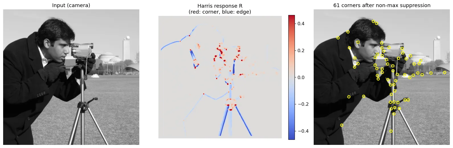

Maximally stable extremal regions (MSER)

Plain version. Imagine slowly flooding a gray-level landscape. Dark letters on bright paper become little lakes. As the water level rises, most lakes grow quickly or merge, but a letter’s lake keeps exactly its shape over a long range of levels, because the ink is much darker than the paper around it. Regions that barely change while the level changes a lot are maximally stable. Matas, Chum, Urban and Pajdla introduced them for wide-baseline stereo [5].

Precise version. Threshold the image at every level $t$. A connected component of $\{f \le t\}$ (or of $\{f \ge t\}$, for bright regions) is an extremal region $Q_t$: every pixel inside is darker (or brighter) than every pixel on its outer boundary. As $t$ increases, the components grow and merge, forming a tree. For each region, define the stability

$$q(t) = \frac{|Q_{t+\Delta} \setminus Q_{t-\Delta}|}{|Q_t|},$$

where $|\cdot|$ is area and $\Delta$ a step in gray levels. A region is maximally stable when $q(t)$ has a local minimum. The whole tree can be built in near-linear time using a union-find structure over pixels sorted by intensity.

Why it works: the definition uses only the order of intensities, so MSERs are invariant to any monotonic change of brightness. Connected regions map to connected regions under continuous geometric changes, so MSERs are covariant with affine transformations (commonly an ellipse is fitted to each region and normalized to a circle before describing it). MSERs work best on well-defined uniform blobs, such as text, signs and windows, and poorly on blurred or highly textured scenes.

import cv2
from skimage import data

img = data.page()                                    # uint8 grayscale
mser = cv2.MSER_create(delta=5, min_area=10, max_area=800, max_variation=0.5)
regions, boxes = mser.detectRegions(img)             # pixel lists + bounding boxes
print(len(regions), "regions")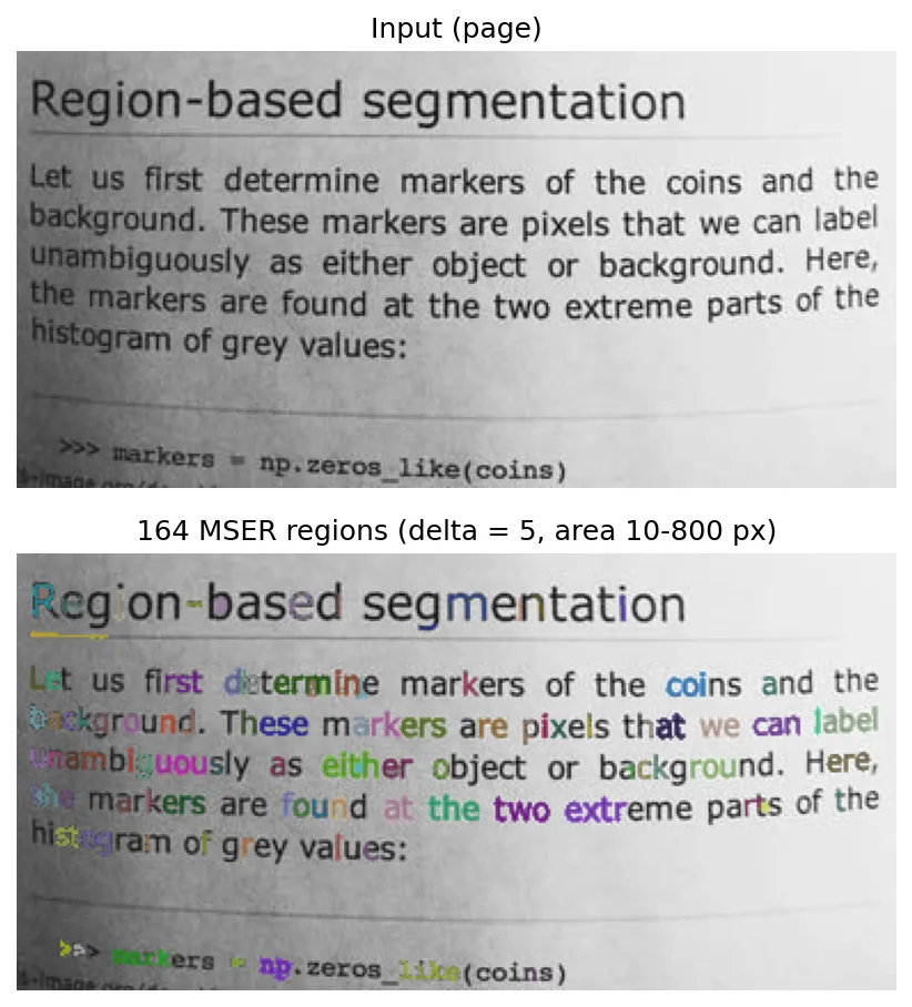

Scale-invariant feature transform (SIFT)

Plain version. SIFT, introduced by Lowe [6], answers three questions about every landmark: where is it, how big is it, and which way is it facing? Then it writes down a summary of the gradients around it, measured in that landmark’s own size and direction, so the summary is the same whether the photo was taken close up, far away, tilted, or in dim light.

Scale space

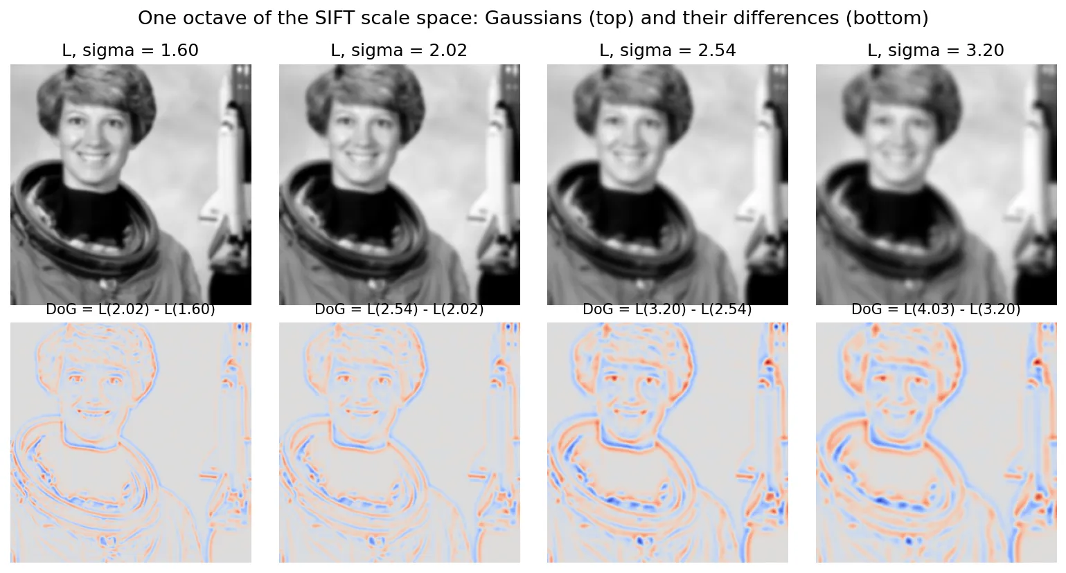
To find features at every size, SIFT builds a scale space: the image blurred by Gaussians of increasing width,

$$L(x, y, \sigma) = G(x, y, \sigma) \star f(x, y), \qquad G(x, y, \sigma) = \frac{1}{2\pi\sigma^2} e^{-(x^2 + y^2)/2\sigma^2},$$

where $\star$ denotes convolution and $\sigma$ the scale. The scales are grouped into octaves; each octave doubles $\sigma$ and is divided into $s$ intervals, so consecutive scales differ by a factor $k = 2^{1/s}$. Lowe [6] uses $s = 3$ and a base scale $\sigma_0 = 1.6$. After each octave the image is downsampled by 2, which keeps the cost low.

Keypoint detection with difference of Gaussians

Adjacent blurred images are subtracted:

$$D(x, y, \sigma) = L(x, y, k\sigma) - L(x, y, \sigma).$$

This difference of Gaussians (DoG) is a close approximation of the scale-normalized Laplacian of Gaussian, $\sigma^2 \nabla^2 G$, scaled by the constant $(k - 1)$. It responds strongly to blobs whose size matches $\sigma$ (Figure 12.7). Candidate keypoints are the pixels whose $D$ value is larger or smaller than all 26 neighbors: 8 in the same DoG image and 9 in each of the scales above and below. A keypoint therefore comes with a position and a characteristic scale.

Keypoint localization

Extrema are found on a discrete grid. To refine them, fit a 3-D quadratic to $D$ around the sample using its Taylor expansion,

$$D(\mathbf{x}) \approx D + \frac{\partial D}{\partial \mathbf{x}}^{\mathsf T} \mathbf{x} + \frac{1}{2}\mathbf{x}^{\mathsf T} \frac{\partial^2 D}{\partial \mathbf{x}^2}\mathbf{x}, \qquad \hat{\mathbf{x}} = -\left(\frac{\partial^2 D}{\partial \mathbf{x}^2}\right)^{-1} \frac{\partial D}{\partial \mathbf{x}},$$

where $\mathbf{x} = (x, y, \sigma)^{\mathsf T}$ is the offset from the sample point and $\hat{\mathbf{x}}$ the sub-pixel, sub-scale location of the extremum. Two tests then remove unstable points [6]:

• Low contrast: discard if $|D(\hat{\mathbf{x}})| < 0.03$ (for intensities in $[0, 1]$).
• Edge responses: DoG also responds along edges, where position is poorly defined. Using the $2 \times 2$ spatial Hessian $\mathbf{H}$ of $D$, keep the point only if

$$\frac{\operatorname{tr}(\mathbf{H})^2}{\det(\mathbf{H})} < \frac{(r + 1)^2}{r},$$

where $r$ bounds the ratio of the two principal curvatures; Lowe uses $r = 10$. This is the same idea as Harris: a good point must curve strongly in both directions.

Orientation assignment

Around each keypoint, compute gradient magnitudes and directions in $L$ at the keypoint’s scale. Build a 36-bin histogram of directions (10° per bin), each sample weighted by its gradient magnitude and by a Gaussian window with $\sigma$ equal to 1.5 times the keypoint scale. The highest peak gives the keypoint’s orientation; any other peak above 80% of the highest creates an additional keypoint with that orientation [6]. From now on, all measurements are made relative to this orientation, which gives rotation invariance.

The keypoint descriptor

Take a window around the keypoint, rotated to its orientation and sized by its scale. Divide it into a $4 \times 4$ grid of cells. In each cell, accumulate an 8-bin histogram of gradient directions, weighted by magnitude and a Gaussian centered on the keypoint, with trilinear interpolation so that small shifts do not cause sudden jumps between bins. This gives $4 \times 4 \times 8 = 128$ numbers [6]. Finally:

1. normalize the vector to unit length (cancels contrast changes $f \mapsto af$; gradients already cancel $+b$),
2. clip every element at 0.2 (limits the influence of a few very large gradients caused by nonlinear lighting such as glare),
3. renormalize to unit length.

Matching

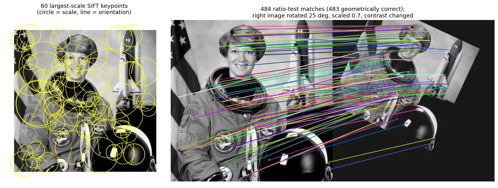
Descriptors from two images are compared by Euclidean distance. The nearest neighbor alone is not reliable: many keypoints have no true match at all. Lowe’s ratio test keeps a match only if

$$\frac{\lVert \mathbf{d} - \mathbf{d}_{1} \rVert}{\lVert \mathbf{d} - \mathbf{d}_{2} \rVert} < \tau,$$

where $\mathbf{d}_1, \mathbf{d}_2$ are the nearest and second-nearest descriptors in the other image and $\tau$ a threshold (Lowe suggests 0.8) [6]. A distinctive match is much closer than the runner-up. Large databases use approximate nearest-neighbor search, and the surviving matches are usually verified geometrically, for example by fitting a similarity, affine, or projective transformation with RANSAC (random sample consensus) [21] and keeping the inliers.

import numpy as np
from skimage import data, feature, transform
from skimage.color import rgb2gray
from skimage.measure import ransac

img1 = rgb2gray(data.astronaut())
tf = transform.AffineTransform(scale=0.7, rotation=np.deg2rad(25), translation=(140, -60))
img2 = 0.8 * transform.warp(img1, tf.inverse) + 0.1        # second "view"

sift = feature.SIFT()
sift.detect_and_extract(img1); k1, d1 = sift.keypoints, sift.descriptors
sift.detect_and_extract(img2); k2, d2 = sift.keypoints, sift.descriptors

matches = feature.match_descriptors(d1, d2, max_ratio=0.6, cross_check=True)  # ratio test
src, dst = k1[matches[:, 0]][:, ::-1], k2[matches[:, 1]][:, ::-1]           # (row, col) -> (x, y)
model, inliers = ransac((src, dst), transform.SimilarityTransform,
                        min_samples=3, residual_threshold=2, max_trials=500)
print(len(matches), "matches,", inliers.sum(), "inliers")
print("recovered scale %.3f, rotation %.1f deg" % (model.scale, np.degrees(model.rotation)))

On this synthetic pair the script finds 484 matches, 483 of them consistent with the true transformation, and recovers scale 0.700 and rotation 25.0°. Real photo pairs, with viewpoint changes, occlusion and repeated patterns, give far lower inlier ratios, which is why geometric verification is not optional.

Modern view

What the surveys say

Shape descriptors. Zhang and Lu’s review [9] sorts shape descriptors along two axes: contour-based versus region-based, and global (one vector for the whole shape) versus structural (the shape broken into primitives). Everything in the first half of this chapter fits that grid: chain codes and polygons are structural contour methods; Fourier descriptors and boundary moments are global contour methods; area, Euler number and Hu moments are global region methods; skeletons are structural region methods. For each technique the review describes the implementation and lists its advantages and disadvantages; the practical message is that no single descriptor is best for every application, so the choice depends on which invariances and how much detail the task needs.

Local feature detectors. Tuytelaars and Mikolajczyk [10] survey interest-point and region detectors: corner detectors (Harris and its scale- and affine-adapted versions), blob detectors (Laplacian/DoG, Hessian), and region detectors (MSER and others). They organize the field around properties a good local feature should have: repeatability, distinctiveness, locality, quantity, accuracy and efficiency. They point out that repeatability, the most important property, can be reached in two ways: by invariance (model large deformations mathematically and design the detector to ignore them) or by robustness (tolerate small ones such as noise, blur and compression). They also note that some properties compete: distinctiveness and locality cannot both be maximized, because a more local feature sees less intensity pattern and is harder to match correctly. Which compromise is right depends on the application. The two speed-oriented descendants of SIFT are good examples of trading accuracy for time: SURF [7] approximates Gaussian derivatives with box filters on integral images, and ORB [8] combines the FAST corner test with an oriented binary descriptor compared by Hamming distance, fast enough for phones.

Texture. Liu et al. [11] review roughly two decades of texture representation for classification, organized into bag-of-words pipelines (local descriptors, coding and pooling), CNN-based methods, and attribute-based methods. Co-occurrence statistics [3] sit at the root of this history: they are the first widely used descriptors of pairs of pixels. The survey, which covers more than 200 publications, traces how the field moved from hand-designed local descriptors encoded as bags of words to representations built on CNN features, and it closes with open questions and directions for future work.

Image matching, handcrafted to deep. Ma et al. [12] follow the full matching pipeline (detection, description, and matching with outlier removal) from handcrafted methods to trainable ones, and compare them experimentally on standard datasets. They show that learning has entered every stage of the pipeline, not only the descriptor. Jin et al. [13] built a benchmark that scores methods by the accuracy of the final camera poses rather than by intermediate metrics. Their key finding is a cautionary one: once each method’s settings (ratio-test threshold, RANSAC parameters, number of keypoints) are tuned properly, classical pipelines such as SIFT can still beat methods perceived as the state of the art, which suggests that some reported gains reflected untuned baselines.

How deep learning changed feature extraction

Learned keypoints and descriptors. SuperPoint [14] trains one fully convolutional network to output both a keypoint heatmap and dense descriptors. It is self-supervised: it first learns corners on synthetic shapes, then improves itself on real images through homographic adaptation, aggregating its own detections over many random warps of the same image. DISK [16] trains detection and description end to end with reinforcement learning (policy gradient), rewarding keypoints that lead to correct matches. These replace the formulas of Harris and SIFT with learned functions, but keep the same idea: sparse, repeatable points with descriptors.

Learned matching. SuperGlue [15] replaces the nearest-neighbor ratio test with a graph neural network that lets keypoints in both images attend to each other, then solves an optimal-transport assignment that can also say “no match”. LightGlue [18] reworks this design to be faster and adaptive, spending less computation on easy image pairs. LoFTR [17] removes the detector altogether: a Transformer with self- and cross-attention matches coarse feature maps densely and then refines positions, which helps in low-texture areas where detectors find nothing.

General-purpose deep features. The deepest change is that features are increasingly not designed for a task at all. Self-supervised foundation models such as DINOv2 [19] produce patch features that work across classification, segmentation, depth estimation and retrieval without fine-tuning. RoMa [20] shows the effect on matching: it uses frozen DINOv2 features for coarse matching, combined with fine convolutional features for precise localization. In other words, the handcrafted descriptor at the center of SIFT has been replaced by a network trained on a very large image collection.

What did not change. The problem decomposition of this chapter survives. Modern pipelines still detect, describe, match and verify geometrically, typically still with a RANSAC-style robust estimator [21]. Scale and rotation still have to be handled, either built in (SIFT’s scale space, ORB’s orientation) or learned from data augmentation. Invariance is still a design choice: a descriptor that is too invariant loses discriminative power, whether it was handcrafted or learned. And in measurement-driven fields (materials, microscopy, quality inspection), region descriptors such as area, circularity, Euler number and GLCM statistics remain popular because each number has a physical meaning a human can check.

Key takeaways

• A detector finds features (points, regions, boundaries); a descriptor turns each into a vector. Detectors should be covariant with geometric changes; descriptors should be invariant to the changes that do not matter for the task.
• Boundaries are first ordered (boundary following) and simplified (chain codes, minimum-perimeter polygons, merging and splitting, signatures, skeletons) before being measured.
• Fourier descriptors compress a closed contour into a few coefficients; dropping $a(0)$, dividing by $|a(1)|$ and keeping magnitudes gives translation, scale, rotation and start-point invariance.
• Region descriptors range from size and shape (area, circularity, eccentricity) to topology (Euler number $E = C - H$), texture (histogram moments, GLCM features, spectral signatures) and Hu’s moment invariants.
• PCA (the Hotelling transform) decorrelates measurements, aligns objects to their principal axes, and gives compact eigen-image descriptors; the error from dropping components equals the sum of the dropped eigenvalues.
• Harris finds corners from the structure tensor; MSER finds regions stable over many thresholds; SIFT adds scale space, orientation and a normalized 128-D gradient histogram, then matches with the ratio test.
• Learned detectors, matchers and foundation-model features are now the focus of most matching research, but carefully tuned classical pipelines remain strong baselines, and the detect–describe–match–verify structure has not changed.

Exercises

1. Chain codes by hand. Write the 8-direction chain code of an axis-aligned $3 \times 2$ rectangle of boundary links (3 links wide, 2 tall), starting at its lower-left corner and walking counterclockwise. Compute its first difference and the shape number (minimum circular rotation). Then rotate the rectangle by 90° and show the shape number does not change.

Hint

Walking counterclockwise from the lower-left corner (with 0 = east, 2 = north): $0\,0\,0\,2\,2\,4\,4\,4\,6\,6$. Each element of the first difference counts counterclockwise turns from the previous direction: $2\,0\,0\,2\,0\,2\,0\,0\,2\,0$ (the leading 2 comes from the wrap-around, $6 \to 0$). Its smallest circular rotation is $0\,0\,2\,0\,2\,0\,0\,2\,0\,2$. After a 90° turn every code element increases by 2 (mod 8), which leaves the differences unchanged.

2. Fourier descriptor invariance, tested. Take the fourier_descriptor function from this chapter. (a) Show numerically that it fails to distinguish a shape from its mirror image. (b) Explain why from the table of transformation effects, and propose a change that would tell mirror images apart.

Hint

Flip the mask with mask[:, ::-1] and trace both contours with find_contours; the descriptors agree to within about $10^{-4}$. A tracer walks every boundary in the same rotational sense, so the mirrored boundary is $s'(k) = \overline{s(-k)}$ (conjugate and reversed), up to a shift. Its DFT is $\overline{a(u)}$: the same magnitudes, opposite phases. Magnitudes cannot see the reflection. Keep some phase instead: the complex number $a(u)\,a(2-u)/a(1)^2$ (indices modulo $K$) is unchanged by translation, rotation, scale and start point, but it is conjugated by a reflection, so the sign of its imaginary part tells a shape from its mirror image.

3. Circularity on a grid. Compute $4\pi A / P^2$ for digital disks of radius 5, 10, 20 and 50 pixels using skimage.draw.disk and regionprops. Why is the result not exactly 1, and how does it change with radius? Try perimeter_crofton as well.

Hint

The digital perimeter is a staircase, and different estimators correct for this differently. Errors are relatively larger for small disks. Report both perimeter estimates; one of them should be noticeably closer to the true $2\pi r$.

4. Texture direction. Create a synthetic texture of horizontal stripes with period 8 pixels plus a little noise. Compute GLCM contrast for offsets of 1 pixel at angles 0°, 45°, 90° and 135°, and the angular spectral signature $S(\theta)$. Which angle stands out in each, and why do the two methods agree?

Hint

Moving along a stripe (0°) keeps intensity almost constant, so contrast is low; moving across stripes (90°) changes it. In the spectrum, horizontal stripes put energy on the vertical frequency axis. Watch the convention: scikit-image’s angle 0 means a horizontal pixel offset.

5. PCA by eigenvalues. For a filled ellipse with semi-axes $a = 40$ and $b = 10$, predict the ratio $\lambda_1 / \lambda_2$ of the coordinate-covariance eigenvalues, then verify it in code. Use your answer to relate $\lambda_1, \lambda_2$ to the eccentricity reported by regionprops.

Hint

For a uniform filled ellipse, the variance along a semi-axis of length $a$ is $a^2/4$. So $\lambda_1 / \lambda_2 = (a/b)^2 = 16$, and $e = \sqrt{1 - \lambda_2/\lambda_1} = \sqrt{1 - b^2/a^2} \approx 0.968$.

6. Ratio test trade-off. Using the SIFT matching script, vary max_ratio from 0.5 to 0.95 and plot (a) the number of matches and (b) the fraction of RANSAC inliers. Then add a 0.6× rescale plus 30° rotation plus Gaussian noise ($\sigma = 0.05$) and repeat. Where would you set the threshold, and why does the answer depend on the noise?

Hint

A loose ratio admits more matches but more of them are wrong; a strict ratio keeps few, mostly correct ones. RANSAC can tolerate many outliers but needs a minimum number of correct matches, so the best threshold sits between the two extremes and moves with image quality.

References

1. R. C. Gonzalez and R. E. Woods, Digital Image Processing, 4th ed., Pearson, 2018, Ch. 12. publisher page
2. M.-K. Hu, “Visual pattern recognition by moment invariants,” IRE Transactions on Information Theory, vol. 8, no. 2, pp. 179–187, 1962. doi
3. R. M. Haralick, K. Shanmugam, and I. Dinstein, “Textural features for image classification,” IEEE Transactions on Systems, Man, and Cybernetics, vol. SMC-3, no. 6, pp. 610–621, 1973. doi
4. C. Harris and M. Stephens, “A combined corner and edge detector,” in Proc. Alvey Vision Conference, pp. 23.1–23.6, 1988. doi
5. J. Matas, O. Chum, M. Urban, and T. Pajdla, “Robust wide-baseline stereo from maximally stable extremal regions,” Image and Vision Computing, vol. 22, no. 10, pp. 761–767, 2004. doi
6. D. G. Lowe, “Distinctive image features from scale-invariant keypoints,” International Journal of Computer Vision, vol. 60, no. 2, pp. 91–110, 2004. doi
7. H. Bay, A. Ess, T. Tuytelaars, and L. Van Gool, “Speeded-up robust features (SURF),” Computer Vision and Image Understanding, vol. 110, no. 3, pp. 346–359, 2008. doi
8. E. Rublee, V. Rabaud, K. Konolige, and G. Bradski, “ORB: An efficient alternative to SIFT or SURF,” in Proc. IEEE International Conference on Computer Vision (ICCV), pp. 2564–2571, 2011. doi
9. D. Zhang and G. Lu, “Review of shape representation and description techniques,” Pattern Recognition, vol. 37, no. 1, pp. 1–19, 2004. doi
10. T. Tuytelaars and K. Mikolajczyk, “Local invariant feature detectors: A survey,” Foundations and Trends in Computer Graphics and Vision, vol. 3, no. 3, pp. 177–280, 2008. doi
11. L. Liu, J. Chen, P. Fieguth, G. Zhao, R. Chellappa, and M. Pietikäinen, “From BoW to CNN: Two decades of texture representation for texture classification,” International Journal of Computer Vision, vol. 127, pp. 74–109, 2019. arXiv
12. J. Ma, X. Jiang, A. Fan, J. Jiang, and J. Yan, “Image matching from handcrafted to deep features: A survey,” International Journal of Computer Vision, vol. 129, pp. 23–79, 2021. doi
13. Y. Jin, D. Mishkin, A. Mishchuk, J. Matas, P. Fua, K. M. Yi, and E. Trulls, “Image matching across wide baselines: From paper to practice,” International Journal of Computer Vision, 2021. doi · arXiv
14. D. DeTone, T. Malisiewicz, and A. Rabinovich, “SuperPoint: Self-supervised interest point detection and description,” arXiv:1712.07629, 2017. arXiv
15. P.-E. Sarlin, D. DeTone, T. Malisiewicz, and A. Rabinovich, “SuperGlue: Learning feature matching with graph neural networks,” arXiv:1911.11763, 2019. arXiv
16. M. J. Tyszkiewicz, P. Fua, and E. Trulls, “DISK: Learning local features with policy gradient,” arXiv:2006.13566, 2020. arXiv
17. J. Sun, Z. Shen, Y. Wang, H. Bao, and X. Zhou, “LoFTR: Detector-free local feature matching with Transformers,” arXiv:2104.00680, 2021. arXiv
18. P. Lindenberger, P.-E. Sarlin, and M. Pollefeys, “LightGlue: Local feature matching at light speed,” arXiv:2306.13643, 2023. arXiv
19. M. Oquab, T. Darcet, T. Moutakanni, et al., “DINOv2: Learning robust visual features without supervision,” arXiv:2304.07193, 2023. arXiv
20. J. Edstedt, Q. Sun, G. Bökman, M. Wadenbäck, and M. Felsberg, “RoMa: Robust dense feature matching,” in Proc. IEEE/CVF Conference on Computer Vision and Pattern Recognition (CVPR), 2024. arXiv
21. M. A. Fischler and R. C. Bolles, “Random sample consensus: A paradigm for model fitting with applications to image analysis and automated cartography,” Communications of the ACM, vol. 24, no. 6, pp. 381–395, 1981. doi