Chapter 13 · Image Pattern Classification

What you’ll learn

• How patterns, pattern vectors and pattern classes turn “what is in this image?” into a precise decision problem
• How prototype matching works: the minimum-distance classifier, correlation-based template matching, SIFT feature matching and matching of structural descriptions
• Why the Bayes classifier is optimal, and what it becomes when each class is Gaussian
• How a perceptron learns, how multilayer networks are trained with backpropagation, and how a convolutional neural network (CNN) learns its own features
• The practical side of training: overfitting, data augmentation and regularization
• How image classification moved from AlexNet to Vision Transformers, CLIP and DINOv2, and why benchmark numbers deserve suspicion

The big picture

Chapters 10–12 carved an image into regions and described each region with numbers: areas, moments, Fourier descriptors, texture statistics, keypoint descriptors. This chapter closes the pipeline. It takes those descriptions and assigns each one a label: “coin”, “digit 7”, “water”, “tumor”, “cat”. Almost every practical vision system ends with such a decision, so this is where image processing meets machine learning.

The chapter follows a historical arc that is also a conceptual one [1]. First come classifiers that work directly with prototypes (a typical member of each class). Then comes the statistically optimal classifier, which needs the class probability distributions. Finally come neural networks, which learn the decision rule from data. In their convolutional form they also learn the features, which removes much of the hand-crafted feature engineering of Chapter 12. If you want a gentle refresher on supervised learning, cost functions and gradient descent first, see the blog post Introduction to Machine Learning.

Background

Plain version. A classifier is a function that looks at a description of something and answers “which group does this belong to?”. We build it from examples whose answers we already know.

A pattern is an arrangement of descriptors that represents an object or region. A pattern class is a family of patterns that share some property. We write the $W$ classes as $\omega_1, \omega_2, \dots, \omega_W$. Pattern recognition by machine means assigning each pattern to its class automatically and with as few mistakes as possible.

The work splits into two stages:

1. Representation. Choose what to measure: pixel values, region descriptors, keypoint descriptors, or learned features. Chapter 12 covered this stage.
2. Decision. Given the measurements, choose a class. This chapter covers this stage.

Methods are usually trained with supervised learning: we have a training set of patterns with known labels and use it to set the classifier’s parameters. We then measure performance on a separate test set that the classifier never saw. A third split, the validation set, is used to choose settings such as the network size or the stopping time. Mixing these sets up is the most common source of over-optimistic results.

A useful way to think about any classifier is through decision functions. For each class $\omega_j$ we define a function $d_j(\mathbf{x})$ and assign $\mathbf{x}$ to the class with the largest value:

$$\mathbf{x} \in \omega_i \quad \text{if} \quad d_i(\mathbf{x}) > d_j(\mathbf{x}) \quad \text{for all } j \neq i .$$

Here $\mathbf{x}$ is the pattern and $d_j$ is a scalar score for class $\omega_j$. The decision boundary between classes $i$ and $j$ is the set where $d_i(\mathbf{x}) - d_j(\mathbf{x}) = 0$. Every classifier in this chapter, from the simplest to a deep network, is a particular way of building these functions.

Patterns and pattern classes

Plain version. We describe objects either with a list of numbers (a vector) or with a description of how their parts connect (a string or a tree).

Pattern vectors

The most common representation is a column vector of $n$ measurements:

$$\mathbf{x} = \begin{bmatrix} x_1 \\ x_2 \\ \vdots \\ x_n \end{bmatrix} ,$$

where each $x_k$ is one descriptor, such as the area of a region, its hue, a moment invariant or the response of a texture filter. A vector is a point in $n$-dimensional feature space. Good features put patterns from the same class close together and patterns from different classes far apart. If the features are poor, no classifier can rescue them.

Two practical points matter here. First, features with different units need normalization; otherwise the one with the largest numeric range dominates any distance. In the fruit example, hue lies in $[0, 1]$ while diameter is measured in centimetres, so we standardize each feature to zero mean and unit variance before comparing distances. Second, the whole image can itself be a pattern vector: an $M \times N$ image flattened into an $MN$-dimensional vector. This is how neural networks see images, and it is why they need so much data, because the space is enormous.

Structural patterns: strings and trees

Some objects are better described by how their parts are arranged than by a list of numbers. A boundary traced as a chain code (Chapter 12) is a string of symbols, for example 0 0 1 2 2 3 .... A scene can be described by a tree: the root is the image, its children are the main regions, and their children are sub-regions. Structural descriptions keep relations such as “is inside”, “is above” or “follows”, which vectors throw away. They are useful for shapes, characters and diagrams, where the order and connection of parts carry the meaning.

Pattern classification by prototype matching

Plain version. Keep one typical example of each class. To classify something new, see which typical example it looks most like.

Minimum-distance classifier

The simplest prototype is the mean vector of each class, computed from its training patterns:

$$\mathbf{m}_j = \frac{1}{n_j} \sum_{\mathbf{x} \in \omega_j} \mathbf{x}, \qquad j = 1, 2, \dots, W ,$$

where $n_j$ is the number of training patterns of class $\omega_j$. A new pattern goes to the class whose mean is nearest in Euclidean distance, $D_j(\mathbf{x}) = \lVert \mathbf{x} - \mathbf{m}_j \rVert$.

Minimizing $D_j^2 = \mathbf{x}^\top\mathbf{x} - 2\mathbf{x}^\top \mathbf{m}_j + \mathbf{m}_j^\top \mathbf{m}_j$ over $j$ is the same as maximizing

$$d_j(\mathbf{x}) = \mathbf{x}^\top \mathbf{m}_j - \tfrac{1}{2}\, \mathbf{m}_j^\top \mathbf{m}_j ,$$

because $\mathbf{x}^\top\mathbf{x}$ does not depend on $j$. This $d_j$ is linear in $\mathbf{x}$. The boundary between classes $i$ and $j$ is

$$d_i(\mathbf{x}) - d_j(\mathbf{x}) = \mathbf{x}^\top(\mathbf{m}_i - \mathbf{m}_j) - \tfrac{1}{2}(\mathbf{m}_i - \mathbf{m}_j)^\top(\mathbf{m}_i + \mathbf{m}_j) = 0 ,$$

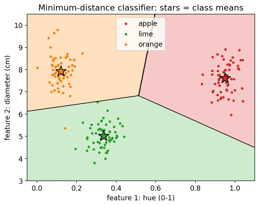
which is the perpendicular bisector of the segment joining $\mathbf{m}_i$ and $\mathbf{m}_j$: a line in 2-D, a plane in 3-D, a hyperplane in general. Figure 13.1 shows the result on our fruit data.

import numpy as np

def fit_min_distance(X, y):
    """X: (n, d) pattern vectors, y: (n,) labels -> class list and mean vectors."""
    classes = np.unique(y)
    M = np.stack([X[y == c].mean(axis=0) for c in classes])
    return classes, M

def predict_min_distance(X, classes, M):
    d2 = ((X[:, None, :] - M[None, :, :]) ** 2).sum(axis=-1)  # (n, W) squared distances
    return classes[d2.argmin(axis=1)]

rng = np.random.default_rng(0)
X = np.r_[rng.normal([0, 0], 1, (100, 2)), rng.normal([4, 3], 1, (100, 2))]
y = np.repeat([0, 1], 100)
classes, M = fit_min_distance(X, y)
print("training accuracy:", (predict_min_distance(X, classes, M) == y).mean())

The classifier works well when classes are compact, roughly round blobs whose means are far apart compared with their spread. It fails when a class is elongated, curved or made of several clusters, because one mean cannot represent it. Two simple extensions help: keep several prototypes per class, or keep all training patterns and use the nearest one (the nearest-neighbor rule).

Matching by correlation (template matching)

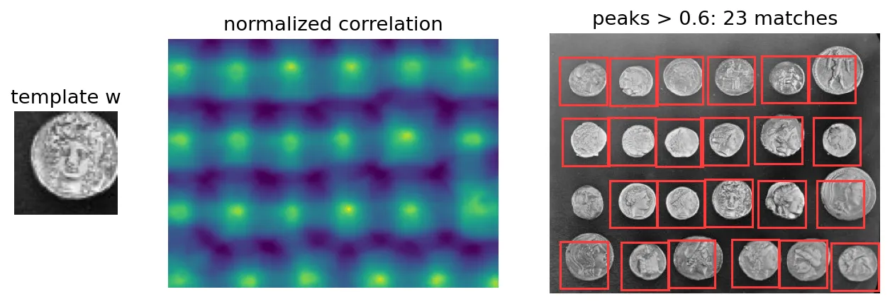
When the prototype is a small image rather than a vector, we compare it with every position of a larger image. This is the 2-D version of prototype matching. Raw correlation $\sum w\,f$ is biased toward bright regions, so we use the normalized correlation coefficient:

$$\gamma(x, y) = \frac{\sum_{s,t} \big[w(s,t) - \bar{w}\big]\big[f(x+s, y+t) - \bar{f}_{xy}\big]} {\sqrt{\sum_{s,t} \big[w(s,t) - \bar{w}\big]^2 \; \sum_{s,t} \big[f(x+s, y+t) - \bar{f}_{xy}\big]^2}} ,$$

where $w$ is the template, $\bar{w}$ its mean, $f$ the image, and $\bar{f}_{xy}$ the mean of the image patch under the template when its corner is at $(x, y)$. The sums run over the template’s support. Because of the subtraction and the division, $\gamma$ lies in $[-1, 1]$ and does not change if the patch’s brightness is scaled or offset. A value of $1$ means a perfect match up to brightness and contrast. Note that this operation is correlation, not convolution: the template is not flipped (see Convolution & Image Filtering).

import cv2
import numpy as np
from skimage import data

img = data.coins().astype(np.float32)
w = img[170:225, 180:235]                            # one coin as the template
R = cv2.matchTemplate(img, w, cv2.TM_CCOEFF_NORMED)  # values in [-1, 1]
y0, x0 = np.unravel_index(R.argmax(), R.shape)
print("best match at", (int(x0), int(y0)), "score", round(float(R.max()), 3))

Figure 13.2 also shows the method’s limits. The template finds almost every coin, because every coin is a bright disk of similar size on a dark background. It cannot tell one coin design from another at this resolution. Correlation is also sensitive to rotation and scale: a template rotated by 30° or enlarged by 30% may no longer produce a clear peak. The usual remedies are to search over a set of rotated and scaled templates, or to match invariant features instead of raw pixels.

Matching SIFT features

The scale-invariant feature transform (SIFT) from Chapter 12 [3] gives exactly those invariant features. Each keypoint has a location, scale, orientation and a 128-dimensional descriptor. To decide whether a prototype object appears in a scene image:

1. Extract keypoints and descriptors from the prototype and from the scene.
2. For each prototype descriptor, find its nearest and second-nearest scene descriptors in Euclidean distance.
3. Accept the match only if the nearest distance is clearly smaller than the second-nearest, for example $d_1 / d_2 < 0.8$. This ratio test [3] rejects ambiguous matches in repetitive texture.
4. Check that the accepted matches agree on one geometric transformation (a similarity, affine or projective map). Matches that disagree are outliers.

The decision is then “object present” if enough geometrically consistent matches survive. This is still prototype matching: the prototype is the set of descriptors, and the “distance” is the number of consistent correspondences. It tolerates rotation, scale change, partial occlusion and moderate viewpoint change, which template matching cannot.

Matching structural prototypes

For strings and trees, the distance must compare symbols and their order. Two simple measures:

• Shape-number similarity. If two closed boundaries are encoded as shape numbers (normalized chain-code differences, Chapter 12), their degree of similarity $k$ is the largest order (code length) at which the two shape numbers are still identical. Similar shapes agree up to high orders. A distance can then be defined as $D = 1/k$: zero for identical shapes, large for shapes that already differ at coarse orders.
• String similarity. Align two strings $a$ and $b$ symbol by symbol. Let $\alpha$ be the number of positions that match and $\beta = \max(|a|, |b|) - \alpha$ the number that do not, where $|a|$ is the length of $a$. Then $R = \alpha / \beta$ is infinite for a perfect match and $0$ when nothing matches. A more forgiving variant is the edit distance: the minimum number of insertions, deletions and substitutions that turns one string into the other, computed by dynamic programming.

A new string goes to the class whose prototype string is most similar. Structural matching is less common today, but the idea of comparing sequences and graphs of parts survives in graph matching and in transformer models that compare sets of tokens.

Optimum (Bayes) statistical classifiers

Plain version. If we know how often each class occurs and what its measurements usually look like, there is a best possible rule: pick the class that is most probable given what we measured. No other rule makes fewer mistakes on average.

Derivation

Let $p(\omega_k \mid \mathbf{x})$ be the probability that pattern $\mathbf{x}$ comes from class $\omega_k$. Let $L_{kj}$ be the loss incurred when a pattern that truly belongs to $\omega_k$ is assigned to $\omega_j$. The expected loss of choosing class $\omega_j$, called the conditional risk, is

$$r_j(\mathbf{x}) = \sum_{k=1}^{W} L_{kj}\, p(\omega_k \mid \mathbf{x}) .$$

Bayes’ rule, $p(\omega_k \mid \mathbf{x}) = p(\mathbf{x} \mid \omega_k)\, P(\omega_k) / p(\mathbf{x})$, rewrites this in terms of the class-conditional density $p(\mathbf{x} \mid \omega_k)$ (what patterns of class $\omega_k$ look like) and the prior $P(\omega_k)$ (how common the class is). The factor $1/p(\mathbf{x})$ is the same for every $j$, so it can be dropped when comparing risks.

The classifier that picks the $j$ with the smallest $r_j(\mathbf{x})$ for every $\mathbf{x}$ minimizes the total average loss. That is why it is called optimal: it is the best any rule can do, given the true distributions. With the common 0–1 loss ($L_{kj} = 0$ if $k = j$, otherwise $1$), every error costs the same and

$$r_j(\mathbf{x}) \propto p(\mathbf{x}) - p(\mathbf{x} \mid \omega_j)P(\omega_j) .$$

Minimizing it means maximizing the decision function

$$d_j(\mathbf{x}) = p(\mathbf{x} \mid \omega_j)\, P(\omega_j) .$$

In words: choose the class with the largest posterior probability. The catch is that we never know the true densities. We must estimate them from training data, and the classifier is only as good as those estimates.

Bayes classifier for Gaussian pattern classes

Assume each class is a multivariate Gaussian with mean $\mathbf{m}_j$ and covariance matrix $\mathbf{C}_j$:

$$p(\mathbf{x} \mid \omega_j) = \frac{1}{(2\pi)^{n/2} \lvert \mathbf{C}_j \rvert^{1/2}} \exp\!\Big[-\tfrac{1}{2}(\mathbf{x} - \mathbf{m}_j)^\top \mathbf{C}_j^{-1} (\mathbf{x} - \mathbf{m}_j)\Big] ,$$

where $n$ is the dimension of $\mathbf{x}$ and $\lvert \mathbf{C}_j \rvert$ the determinant of $\mathbf{C}_j$. Because the logarithm is increasing, we can maximize $\ln d_j$ instead and drop the constant $\tfrac{n}{2}\ln 2\pi$:

$$d_j(\mathbf{x}) = \ln P(\omega_j) - \tfrac{1}{2}\ln \lvert \mathbf{C}_j \rvert - \tfrac{1}{2}(\mathbf{x} - \mathbf{m}_j)^\top \mathbf{C}_j^{-1} (\mathbf{x} - \mathbf{m}_j) .$$

The last term is half the squared Mahalanobis distance, a distance that stretches space so that each class’s spread looks round. This $d_j$ is quadratic in $\mathbf{x}$, so boundaries between classes are quadrics: ellipses, parabolas or hyperbolas in 2-D. Two special cases connect back to earlier sections:

• Equal covariances ($\mathbf{C}_j = \mathbf{C}$ for all $j$). The quadratic term $\mathbf{x}^\top \mathbf{C}^{-1} \mathbf{x}$ is common to all classes and cancels, leaving a linear function $d_j(\mathbf{x}) = \ln P(\omega_j) + \mathbf{x}^\top \mathbf{C}^{-1} \mathbf{m}_j - \tfrac{1}{2}\mathbf{m}_j^\top \mathbf{C}^{-1} \mathbf{m}_j$. Boundaries become hyperplanes.
• Identity covariance and equal priors ($\mathbf{C} = \mathbf{I}$, $P(\omega_j) = 1/W$). The function reduces to $\mathbf{x}^\top \mathbf{m}_j - \tfrac{1}{2}\mathbf{m}_j^\top \mathbf{m}_j$: the minimum-distance classifier. So minimum distance is the Bayes-optimal rule for round, equally spread, equally likely Gaussian classes, and only then.

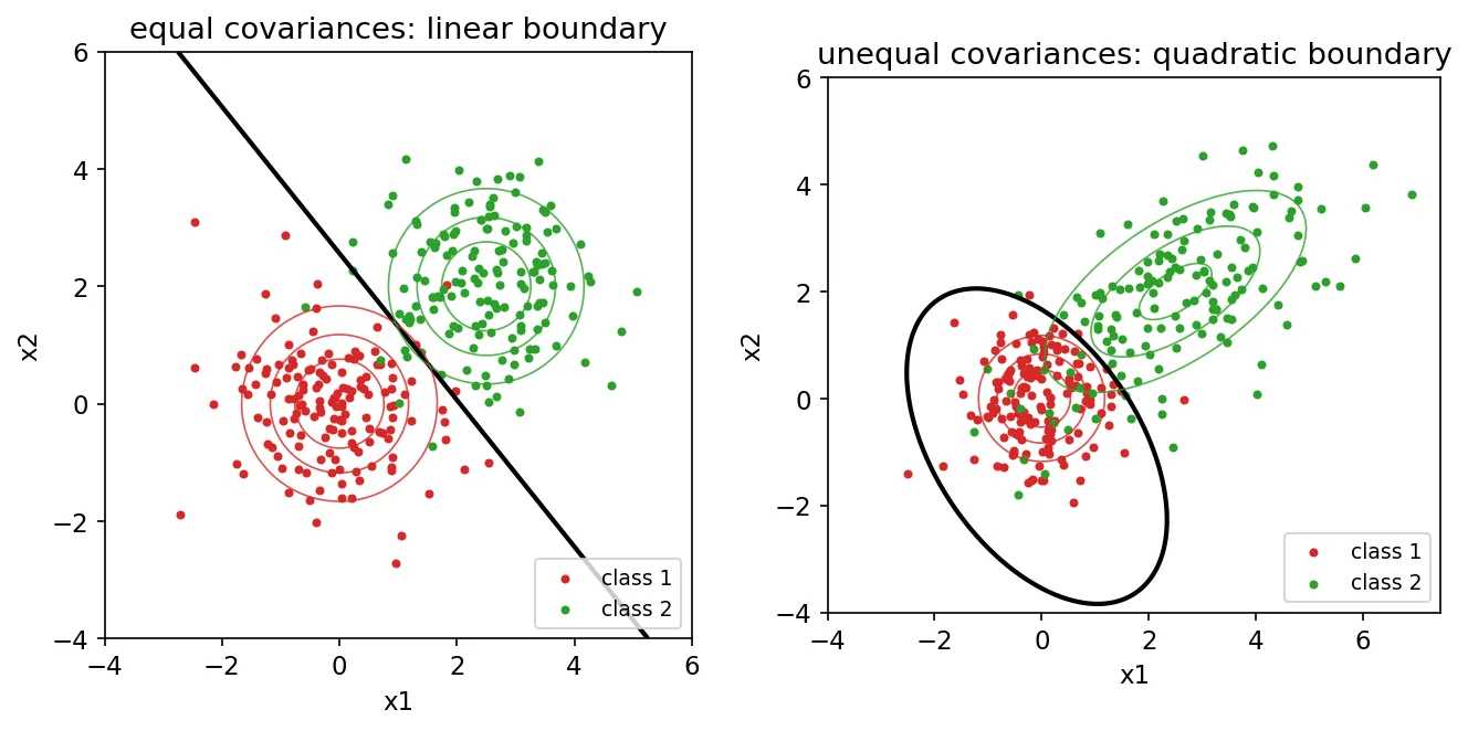
Estimating $\mathbf{m}_j$ and $\mathbf{C}_j$ from samples is easy: the sample mean and sample covariance. The priors can be the class frequencies in the training set, if those reflect reality.

import numpy as np

class GaussianBayes:
    def fit(self, X, y):
        self.classes = np.unique(y)
        self.m = [X[y == c].mean(0) for c in self.classes]
        self.C = [np.cov(X[y == c].T) for c in self.classes]
        self.logP = [np.log((y == c).mean()) for c in self.classes]
        return self

    def decision(self, X):
        scores = []
        for m, C, lp in zip(self.m, self.C, self.logP):
            d = X - m
            maha = np.einsum("ni,ij,nj->n", d, np.linalg.inv(C), d)
            scores.append(lp - 0.5 * np.linalg.slogdet(C)[1] - 0.5 * maha)
        return np.stack(scores, axis=1)            # (n, W): one d_j(x) per class

    def predict(self, X):
        return self.classes[self.decision(X).argmax(1)]

The number of covariance parameters grows as $n(n+1)/2$ per class. With 4 features that is 10 numbers per class, easily estimated. With 1,000 features it is about half a million, and the estimate becomes unreliable unless there is a huge amount of data. This is one reason the Gaussian Bayes classifier works best on short, well-chosen feature vectors.

Application: classifying pixels in a multispectral image

Remote-sensing satellites record each ground location in several spectral bands. Each pixel is then a natural pattern vector, $\mathbf{x} = (x_{\text{blue}}, x_{\text{green}}, x_{\text{red}}, x_{\text{NIR}})^\top$, where NIR is near-infrared. Healthy vegetation reflects strongly in NIR and weakly in red; water is dark in NIR; built-up areas are moderately bright everywhere.

We built a synthetic $128 \times 128$ scene with three classes (water, vegetation, built-up), gave each class a mean reflectance in four bands, and added independent Gaussian noise with standard deviation $0.06$ to every band. We picked only 50 random pixels per class as training data, estimated $\mathbf{m}_j$ and $\mathbf{C}_j$, and classified every pixel with the Gaussian Bayes rule.

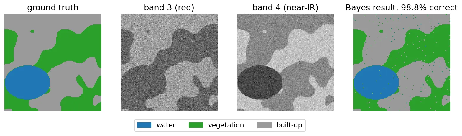
Two lessons stand out. First, no single band is enough: in the red band, water and vegetation have similar values. The combination of bands separates them. Second, the remaining errors are isolated pixels. The Bayes rule here treats each pixel independently and ignores neighbors. Adding spatial context, for example by smoothing the decision scores or using a classifier that sees a neighborhood, removes most of those errors. That observation leads naturally to convolutional networks.

Neural networks and deep learning

Plain version. A neural network is a stack of very simple units. Each unit adds up its inputs with weights, then decides how strongly to “fire”. By nudging the weights after each mistake, the network learns a decision rule on its own, without our writing down the probability distributions.

Background

The Bayes classifier needs density estimates, which are hard to get in high dimensions. An alternative is to learn the decision functions directly from training data. Neural networks do this with many simple, adjustable computing elements arranged in layers. The idea goes back to the perceptron of the late 1950s [4]. It became practical for multilayer networks once backpropagation was popularized in 1986 [5], and it became dominant for images after deep convolutional networks won the ImageNet challenge in 2012 [7]. For a compact Chinese-language summary of perceptrons, MLPs, activation functions and training tricks, see the blog notes 機器學習及類神經網路筆記 (in Traditional Chinese).

The perceptron

A perceptron computes a weighted sum of its inputs plus a bias and outputs the sign:

$$d(\mathbf{x}) = \mathbf{w}^\top \mathbf{x} + w_0 = \sum_{k=1}^{n} w_k x_k + w_0, \qquad \text{class} = \begin{cases} \omega_1 & d(\mathbf{x}) > 0 \\ \omega_2 & d(\mathbf{x}) \le 0 \end{cases}$$

where $\mathbf{w} = (w_1, \dots, w_n)^\top$ are the weights and $w_0$ is the bias. The boundary $d(\mathbf{x}) = 0$ is a hyperplane. To simplify notation, append a constant $1$ to every pattern, $\mathbf{y} = (x_1, \dots, x_n, 1)^\top$, and fold the bias into the weights, $\mathbf{w} = (w_1, \dots, w_n, w_0)^\top$, so that $d = \mathbf{w}^\top \mathbf{y}$.

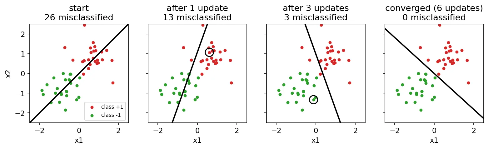
Learning rule. Encode the label as $t = +1$ for $\omega_1$ and $t = -1$ for $\omega_2$. Present the training patterns one at a time. At step $k$:

$$\mathbf{w}(k+1) = \begin{cases} \mathbf{w}(k) + \alpha\, t\, \mathbf{y}(k) & \text{if } t\, \mathbf{w}(k)^\top \mathbf{y}(k) \le 0 \ \text{(misclassified)} \\ \mathbf{w}(k) & \text{otherwise,} \end{cases}$$

where $\alpha > 0$ is the learning rate. Each correction moves the hyperplane so that the offending pattern is pushed toward its correct side: after the update, $t\,\mathbf{w}^\top\mathbf{y}$ increases by $\alpha \lVert \mathbf{y} \rVert^2$. If the two classes are linearly separable, this procedure is guaranteed to stop after a finite number of corrections with a separating hyperplane. If they are not, it never settles. In that case we instead minimize a smooth error, such as the squared difference between $\mathbf{w}^\top \mathbf{y}$ and $t$, by gradient descent (the least-mean-squares, or delta, rule). That idea leads directly to backpropagation.

import numpy as np

def train_perceptron(X, y, alpha=0.5, epochs=100):
    """X: (n, d), y in {-1, +1}. Returns augmented weights (w_1..w_d, w_0)."""
    Xa = np.c_[X, np.ones(len(X))]                 # append the constant input 1
    w = np.zeros(Xa.shape[1])
    for _ in range(epochs):
        mistakes = 0
        for xi, yi in zip(Xa, y):
            if yi * (w @ xi) <= 0:                 # wrong side (or on the line)
                w += alpha * yi * xi
                mistakes += 1
        if mistakes == 0:                          # a full clean pass: converged
            break
    return w

A single perceptron can only draw one hyperplane. It cannot solve XOR, where the two classes sit on opposite corners of a square. To draw curved or multi-piece boundaries we need more layers.

Multilayer feedforward networks

A multilayer feedforward network (or multilayer perceptron, MLP) stacks layers of units. Layer $\ell$ receives the outputs of layer $\ell - 1$, and nothing flows backward during prediction. Unlike the perceptron, each unit passes its weighted sum through a smooth, differentiable activation function $h$, such as the sigmoid $h(z) = 1/(1+e^{-z})$, the hyperbolic tangent, or the rectified linear unit $\text{ReLU}(z) = \max(0, z)$. Smoothness is what makes gradient-based training possible. Nonlinearity is what makes depth useful: a stack of purely linear layers collapses into one linear layer.

With two hidden layers and enough units, a network can form decision regions of essentially any shape. In practice the question is not whether a network can represent a boundary, but whether training will find it from the data available.

Forward pass

Number the layers $\ell = 1, \dots, L$, with layer $0$ being the input $\mathbf{a}^{(0)} = \mathbf{x}$. For each layer,

$$\mathbf{z}^{(\ell)} = \mathbf{W}^{(\ell)} \mathbf{a}^{(\ell-1)} + \mathbf{b}^{(\ell)}, \qquad \mathbf{a}^{(\ell)} = h\big(\mathbf{z}^{(\ell)}\big),$$

where $\mathbf{W}^{(\ell)}$ is the weight matrix (row $i$ holds the weights into unit $i$), $\mathbf{b}^{(\ell)}$ the bias vector, $\mathbf{z}^{(\ell)}$ the net inputs and $\mathbf{a}^{(\ell)}$ the activations, with $h$ applied element by element. For a $W$-class problem the output layer has $W$ units. Its net inputs are turned into probabilities with the softmax function,

$$p_j = \frac{e^{z_j^{(L)}}}{\sum_{i=1}^{W} e^{z_i^{(L)}}}, \qquad j = 1, \dots, W ,$$

and the predicted class is the one with the largest $p_j$. Notice that the output layer is a set of decision functions $d_j(\mathbf{x}) = z^{(L)}_j$, exactly as in the Background section. The hidden layers compute features in which those simple, linear decision functions suffice.

Backpropagation

Training adjusts all weights to reduce a loss $E$ that measures how wrong the outputs are. For classification the standard choice is the cross-entropy $E = -\sum_j t_j \ln p_j$, where $\mathbf{t}$ is the one-hot label (1 for the true class, 0 elsewhere). For a sigmoid output the classic alternative is the squared error $E = \tfrac{1}{2}\lVert \mathbf{a}^{(L)} - \mathbf{t} \rVert^2$. We need $\partial E / \partial \mathbf{W}^{(\ell)}$ for every layer. Backpropagation computes all of them with one backward sweep of the chain rule [5].

Define the error signal of layer $\ell$ as $\boldsymbol{\delta}^{(\ell)} = \partial E / \partial \mathbf{z}^{(\ell)}$.

Step 1: output layer. For softmax with cross-entropy the derivative is remarkably simple:

$$\boldsymbol{\delta}^{(L)} = \mathbf{p} - \mathbf{t} .$$

(For a sigmoid output with squared error it is $(\mathbf{a}^{(L)} - \mathbf{t}) \odot h'(\mathbf{z}^{(L)})$, where $\odot$ is element-wise multiplication.)

Step 2: propagate backward. Unit $i$ of layer $\ell$ affects $E$ only through the net inputs of layer $\ell+1$, and $\partial z^{(\ell+1)}_k / \partial a^{(\ell)}_i = W^{(\ell+1)}_{ki}$. The chain rule gives

$$\boldsymbol{\delta}^{(\ell)} = h'\big(\mathbf{z}^{(\ell)}\big) \odot \Big(\mathbf{W}^{(\ell+1)\top} \boldsymbol{\delta}^{(\ell+1)}\Big), \qquad \ell = L-1, \dots, 1 .$$

The errors travel backward through the same weights that carried the signal forward, transposed.

Step 3: gradients. Because $z^{(\ell)}_i = \sum_k W^{(\ell)}_{ik} a^{(\ell-1)}_k + b^{(\ell)}_i$,

$$\frac{\partial E}{\partial \mathbf{W}^{(\ell)}} = \boldsymbol{\delta}^{(\ell)} \, \mathbf{a}^{(\ell-1)\top}, \qquad \frac{\partial E}{\partial \mathbf{b}^{(\ell)}} = \boldsymbol{\delta}^{(\ell)} .$$

Each weight’s gradient is “error at its output end” times “activation at its input end”.

Step 4: update. Gradient descent with learning rate $\alpha$:

$$\mathbf{W}^{(\ell)} \leftarrow \mathbf{W}^{(\ell)} - \alpha \frac{\partial E}{\partial \mathbf{W}^{(\ell)}}, \qquad \mathbf{b}^{(\ell)} \leftarrow \mathbf{b}^{(\ell)} - \alpha \frac{\partial E}{\partial \mathbf{b}^{(\ell)}} .$$

The cost of the backward pass is about the same as the forward pass, which is why networks with millions of weights can be trained at all. The perceptron rule is the special case of one layer with a step activation.

Training

In practice we average the gradient over a small random mini-batch of training patterns, update, and repeat. This is stochastic gradient descent (SGD). One pass through the whole training set is an epoch. Training runs for many epochs while we watch the loss on the validation set. The learning rate is the most important setting: too large and the loss oscillates or explodes; too small and training crawls. Weights must start as small random numbers, not zeros, or all units in a layer would compute the same thing and receive the same updates forever.

The following NumPy program trains a two-layer network on XOR, the problem a single perceptron cannot solve:

import numpy as np

rng = np.random.default_rng(0)
X = np.array([[0, 0], [0, 1], [1, 0], [1, 1]], float)
y = np.array([[0], [1], [1], [0]], float)         # XOR: not linearly separable

W1, b1 = rng.normal(0, 1, (2, 8)), np.zeros(8)    # input -> 8 hidden units
W2, b2 = rng.normal(0, 1, (8, 1)), np.zeros(1)    # hidden -> 1 output
sig = lambda z: 1 / (1 + np.exp(-z))
alpha = 1.0

for step in range(5000):
    # forward pass
    a1 = np.tanh(X @ W1 + b1)
    out = sig(a1 @ W2 + b2)
    # backward pass (cross-entropy loss with a sigmoid output)
    d2 = (out - y) / len(X)                        # delta at the output layer
    d1 = (d2 @ W2.T) * (1 - a1 ** 2)               # delta at the hidden layer
    W2 -= alpha * a1.T @ d2;  b2 -= alpha * d2.sum(0)
    W1 -= alpha * X.T @ d1;   b1 -= alpha * d1.sum(0)

print(out.round(3).ravel())                        # close to [0, 1, 1, 0]

(Here patterns are rows, so the matrix products are transposed relative to the equations above.)

Deep convolutional neural networks

Plain version. Instead of telling the network which features to measure, we let it slide small learnable filters over the image, exactly like the filters of Chapter 3, and learn which filters help it classify. Early layers end up finding edges and blobs; later layers combine them into parts and whole objects.

Why fully connected networks struggle with images

Feed a $20 \times 20$ image into a fully connected layer with 2,048 hidden units, and that one layer has $400 \times 2048 = 819{,}200$ weights. The layer also ignores the fact that nearby pixels are related and that a “3” shifted two pixels to the right is still a “3”. A CNN builds both facts into its structure [6].

Convolutional layers

A convolutional layer applies $F$ small kernels (for example $5 \times 5$) to its input. With $C$ input channels $a_c$, the net input of output channel $f$ at pixel $(x, y)$ is

$$z_f(x, y) = \sum_{c=1}^{C} \sum_{s,t} w_{f,c}(s, t)\, a_c(x+s, y+t) + b_f ,$$

followed by an activation, usually ReLU: $a_f(x,y) = \max(0, z_f(x,y))$. The sum is a spatial correlation, as in Chapter 3, but the kernel values $w_{f,c}$ are learned. Each output channel is a feature map: it is large where its kernel’s pattern appears. Two ideas cut the parameter count dramatically:

• Local connectivity. Each output depends only on a small neighborhood (its receptive field).
• Weight sharing. The same kernel is used at every position, so a feature learned in one place is detected everywhere.

Eight $5 \times 5$ kernels on a single-channel image need $8 \times 25 + 8 = 208$ parameters, against the 819,200 above.

Pooling layers

A pooling layer shrinks each feature map, typically by taking the maximum (max-pooling) or average of each non-overlapping $2 \times 2$ block. It halves the width and height, makes the response tolerant to small shifts, and enlarges the receptive field of later layers. Stacking convolution and pooling several times yields features that respond to larger and more abstract structures.

Fully connected layers and the whole pipeline

After the last pooling layer the feature maps are flattened into one vector and passed through one or more fully connected layers ending in a softmax. Figure 13.6 shows the small network we trained.

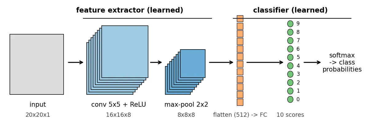
This is the key conceptual point of the chapter. The classical pipeline was hand-designed features → classifier. A CNN is learned features → classifier, with both parts trained together by backpropagation to minimize the same loss. The fully connected softmax layer at the end is just a set of linear decision functions, the same object we met in the minimum-distance and equal-covariance Bayes classifiers. What changed is that the space in which those linear functions operate is itself learned.

Training a CNN

Backpropagation works unchanged; only the local derivatives differ:

• Convolution. Because a weight is shared over all positions, its gradient is the sum over positions: $\partial E/\partial w_{f,c}(s,t) = \sum_{x,y} \delta_f(x,y)\, a_c(x+s, y+t)$, which is itself a correlation of the input with the error map. The error sent back to the input is a convolution of $\delta_f$ with the (flipped) kernel.
• Max-pooling. The gradient flows only to the input that was the maximum in each block; the others get zero.
• ReLU. The gradient passes where $z > 0$ and is blocked where $z \le 0$.

Here is the forward pass of one convolution, ReLU and pooling stage with SciPy:

import numpy as np
from scipy.signal import correlate2d
from skimage import data, transform

img = transform.resize(data.camera(), (64, 64), anti_aliasing=True)
k = np.array([[-1, 0, 1], [-2, 0, 2], [-1, 0, 1]], float)    # one 3x3 "filter"
fmap = np.maximum(correlate2d(img, k, mode="valid") + 0.0, 0)  # conv + bias + ReLU
pooled = fmap[:62, :62].reshape(31, 2, 31, 2).max(axis=(1, 3))  # 2x2 max-pooling
print(img.shape, "->", fmap.shape, "->", pooled.shape)

Worked example: digits

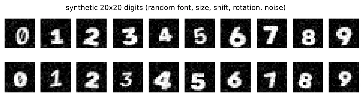
The classic test bed for CNNs is handwritten digit recognition, where LeNet-style networks were developed on the MNIST digits [6]. To keep everything self-contained and reproducible, we generate MNIST-like $20 \times 20$ digits: each digit 0–9 is drawn with one of six OpenCV fonts at a random size, stroke width, shift and rotation (±15°), then noise is added (Figure 13.7).

The network of Figure 13.6 (eight $5 \times 5$ filters, ReLU, $2 \times 2$ max-pooling, a fully connected layer to 10 outputs, softmax with cross-entropy) is written in about 80 lines of NumPy in scripts/figures/dip_ch13.py. We trained it with mini-batch SGD (batch size 32, learning rate 0.05, small weight decay) on 3,000 digits for 12 epochs. It reached 98.5% accuracy on 1,000 separate validation digits. Figure 13.8 shows what it learned.

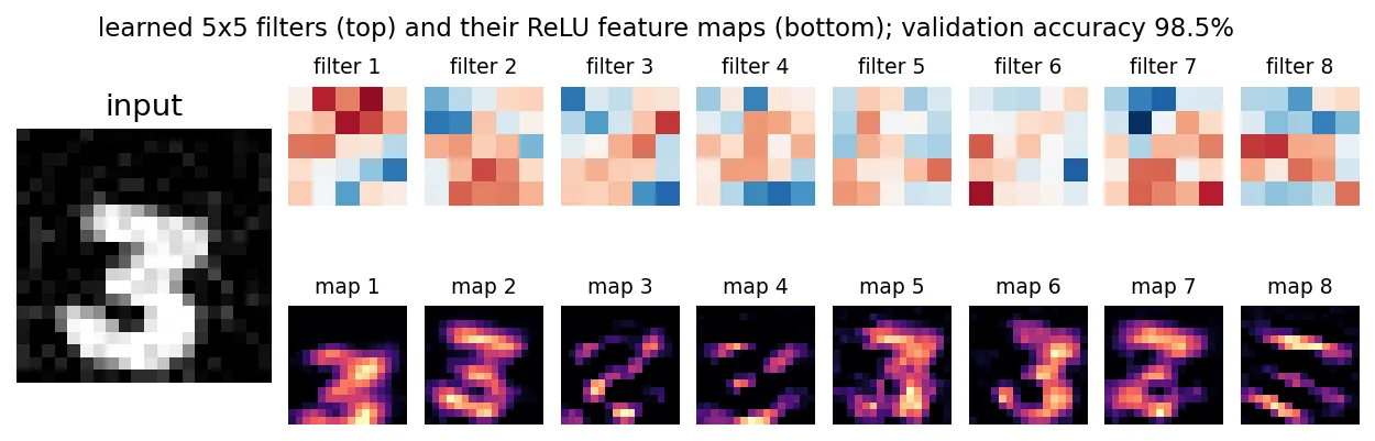
Nobody told the network to detect edges. Oriented, edge-like kernels emerge because they are useful for telling digits apart. Large networks trained on natural images show the same behavior in their first layer, with progressively more complex patterns in deeper layers.

Some additional details of implementation

Plain version. A network that memorizes its homework can still fail the exam. Most of the practical craft of training is about making it learn the general rule instead of the specific examples.

Overfitting

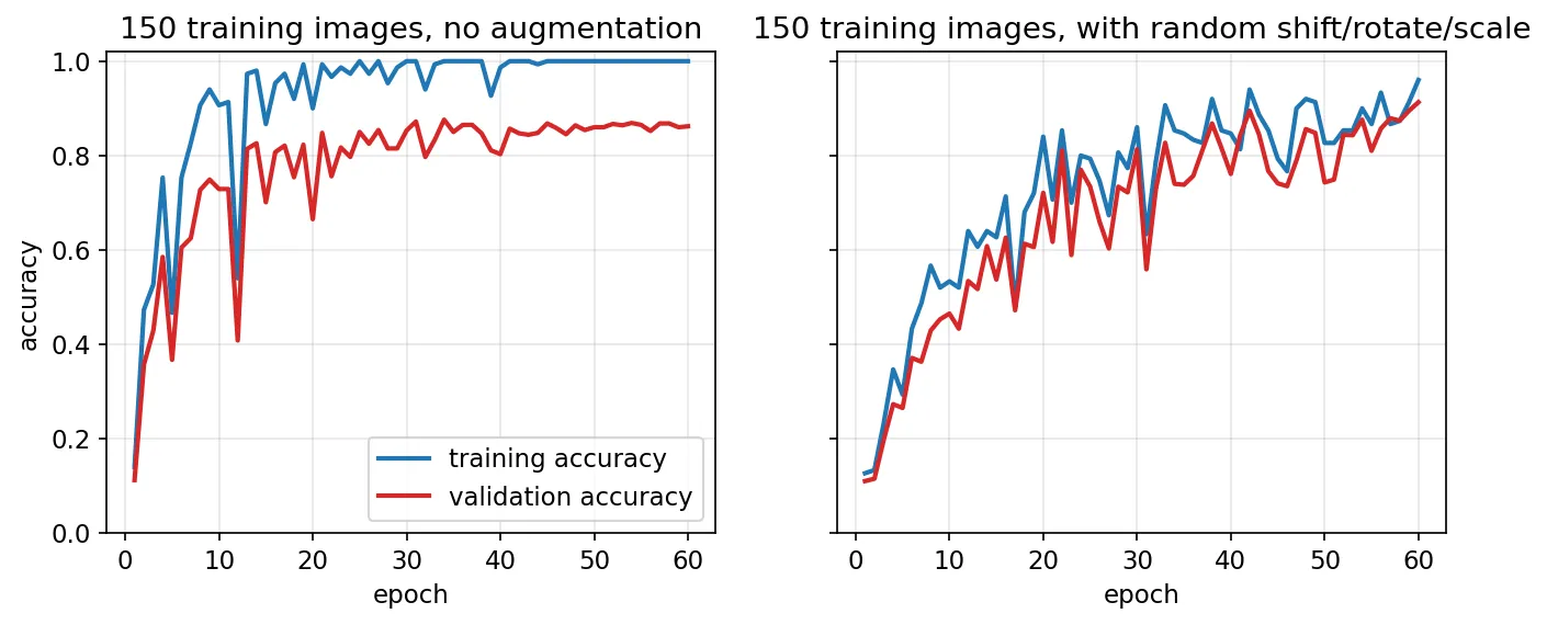
A network with many parameters and few training examples can drive its training error to zero by memorizing. Its error on new data then stays high. This gap between training and validation performance is overfitting. Figure 13.9 (left) shows it clearly: trained on only 150 digits, the CNN reaches 100% training accuracy but only 86.2% validation accuracy.

The basic defenses:

• More data. Nothing helps as reliably. Data augmentation (below) is a cheap way to get more.
• A validation set and early stopping. Track validation accuracy and keep the weights from the best epoch.
• Smaller or better-structured models. Weight sharing in CNNs is itself a strong regularizer compared with fully connected layers.

Data augmentation

Data augmentation creates new training examples by applying label-preserving transformations: small shifts, rotations, scaling, flips (where they make sense: a flipped “cat” is still a cat, but a flipped “b” becomes a “d”), crops, brightness and contrast changes, and added noise [18]. Each epoch sees a slightly different version of each image, so memorizing is harder and invariance to those transformations is learned from data.

Regularization

Regularization adds a preference for simpler solutions:

• Weight decay ($L_2$ regularization) adds $\tfrac{\lambda}{2}\sum w^2$ to the loss, which adds $\lambda w$ to every weight’s gradient and shrinks weights toward zero. Our training script uses $\lambda = 10^{-4}$.
• Dropout randomly sets a fraction of the units to zero at each training step, so no unit can rely on specific partners. At test time all units are used, with appropriately scaled weights. This behaves like averaging an ensemble of many thinned networks [17].

Other practical details matter just as much: normalizing inputs (zero mean, unit variance), initializing weights with a variance scaled to the number of inputs (so activations neither explode nor vanish through the layers), lowering the learning rate during training, and always reporting final results on a test set that was not used for any decision during development.

Modern view

The textbook chapter ends where modern image classification begins. Six survey and review papers map how the field has moved since.

Statistical pattern recognition before deep learning. Jain, Duin and Mao’s review [2] is still the clearest map of the classical territory: representation, feature extraction and selection, Bayes and nearest-neighbor rules, linear and nonlinear classifiers, classifier combination, and error estimation. Its main takeaway, that the feature representation and the evaluation protocol matter more than the choice of classifier, aged well. Deep learning did not refute it; it automated the representation part.

The CNN era. Rawat and Wang [11] review CNNs for image classification from their origins in the late 1980s to 2017, organizing more than 300 papers by architecture, regularization, optimization and practical tricks. The line they trace starts with LeCun et al.’s gradient-trained networks for document recognition [6]. It accelerates with AlexNet [7], which used GPUs, ReLU, dropout and data augmentation to win the ImageNet Large Scale Visual Recognition Challenge in 2012 [10]. VGG [8] showed that depth built from small $3 \times 3$ kernels helps. ResNet [9] made very deep networks trainable by learning residual functions through identity shortcut connections. Each of these is still recognizably the architecture of Figure 13.6: convolution, nonlinearity, pooling, a linear classifier, trained by backpropagation.

Transformers in vision. The Vision Transformer (ViT) [12] cuts an image into $16 \times 16$ patches, treats each patch as a token and processes the sequence with self-attention instead of convolution. With enough pre-training data it matches or exceeds CNNs. Khan et al.’s survey [13] covers the many vision transformer variants for classification, detection, segmentation and more, and discusses their dependence on large-scale pre-training. ConvNeXt [14] then showed that a pure CNN, modernized step by step with design choices borrowed from transformers, is competitive again. The practical lesson: architecture families matter less than training data, scale and recipe.

Foundation features and zero-shot classification. Two 2021–2023 developments changed what “training a classifier” means. CLIP [15] trains an image encoder and a text encoder together so that matching image–caption pairs have similar embeddings. A new classifier can then be built without any labelled images: embed prompts such as a photo of a {class}, and assign each image to the class whose text embedding is most similar. That is a minimum-distance classifier whose prototypes come from language. DINOv2 [16] learns general-purpose visual features by self-supervision on a large curated image set, without labels. Its frozen features support strong classification with only a linear layer or a nearest-neighbor rule on top. In both cases the expensive part, the feature extractor, is trained once. The classifier on top is often one of the simple rules from the first half of this chapter.

Data augmentation and regularization. Shorten and Khoshgoftaar’s survey [18] organizes augmentation methods into basic image manipulations (geometric and color transformations, kernel filters, mixing images, random erasing) and learned approaches (adversarial training, GAN-based synthesis, neural style transfer, meta-learning of augmentation policies). Its takeaway matches Figure 13.9: augmentation is one of the cheapest and most effective ways to reduce overfitting when labelled data are limited.

Evaluation pitfalls and dataset bias. Torralba and Efros [19] asked a simple question: can a classifier tell which dataset an image came from? It could, well above chance, showing that each benchmark has its own “signature”. Models trained on one dataset also generalized poorly to another. Liu and He [20] repeated the experiment with modern networks and very large, diverse web-scale datasets. Modern networks still identify the source dataset with high accuracy on held-out images, and they do it with generalizable features rather than memorization. Dataset bias did not disappear with scale. Two practical consequences follow. Accuracy on one benchmark is a statement about that benchmark, not about the visual world. And whenever possible, test on data collected independently of the training data.

What changed and what did not. Deep learning replaced hand-crafted features and made the classifier itself almost an afterthought: a linear softmax layer. It did not change the decision-theoretic foundations. The softmax output is trained to estimate posterior probabilities, so the network approximates the Bayes rule. Cross-entropy is the negative log-likelihood. Prototype matching survives as nearest-neighbor search in embedding spaces, used in zero-shot classification and retrieval. Template matching by normalized correlation is still the right tool in controlled industrial inspection, where the object’s appearance is fixed and training data are scarce. Understanding the classical methods tells you what the modern ones are optimizing and when a simpler method is enough.

Key takeaways

• Classification assigns a label to a pattern via decision functions $d_j(\mathbf{x})$; the boundaries are where two decision functions are equal.
• Minimum-distance classification uses class means as prototypes; its boundaries are perpendicular bisectors. Normalized correlation and SIFT matching are prototype matching for images and keypoints.
• The Bayes classifier minimizes the average loss. For Gaussian classes it is quadratic; with equal covariances it is linear; with identity covariance and equal priors it reduces to minimum distance.
• A perceptron learns a separating hyperplane by correcting mistakes. Multilayer networks with smooth activations learn nonlinear boundaries, and backpropagation computes all gradients in one backward pass.
• A CNN is a learned feature extractor (convolution, nonlinearity, pooling) followed by a learned linear classifier. Weight sharing makes it efficient and shift-tolerant.
• Overfitting is the central practical risk. Use validation data, data augmentation, weight decay and dropout, and keep the test set untouched.
• Modern systems often pair a large pre-trained feature extractor (CLIP, DINOv2) with a very simple classifier. Benchmark accuracy reflects dataset biases, so test on independently collected data.

Exercises

1. Bisector by hand. Two class means are $\mathbf{m}_1 = (1, 2)^\top$ and $\mathbf{m}_2 = (5, 4)^\top$. Write the minimum-distance boundary $d_1(\mathbf{x}) - d_2(\mathbf{x}) = 0$ as an equation in $x_1, x_2$, and verify that the midpoint of the two means lies on it.

Hint

$\mathbf{m}_1 - \mathbf{m}_2 = (-4, -2)^\top$ and $\tfrac{1}{2}(\mathbf{m}_1 - \mathbf{m}_2)^\top(\mathbf{m}_1 + \mathbf{m}_2) = \tfrac{1}{2}(-4 \cdot 6 - 2 \cdot 6) = -18$. The boundary is $-4x_1 - 2x_2 + 18 = 0$, i.e. $2x_1 + x_2 = 9$. The midpoint $(3, 3)$ gives $6 + 3 = 9$. ✓

2. When priors matter. In a one-dimensional problem, class $\omega_1$ is Gaussian with mean 0 and class $\omega_2$ with mean 4, both with variance 1. Find the Bayes threshold when $P(\omega_1) = P(\omega_2)$, and when $P(\omega_1) = 0.9$. In which direction does the threshold move, and why does that make sense?

Hint

Set $\ln P_1 - \tfrac{1}{2}x^2 = \ln P_2 - \tfrac{1}{2}(x-4)^2$. This gives $x = 2 + \tfrac{1}{4}\ln(P_1/P_2)$. Equal priors give $x = 2$; $P_1 = 0.9$ gives $x = 2 + \tfrac{1}{4}\ln 9 \approx 2.55$. The threshold moves toward the rarer class, so more ambiguous patterns go to the common class.

3. Correlation invariance. Show that the normalized correlation coefficient $\gamma$ is unchanged if every pixel of the image patch is replaced by $a f + b$ with $a > 0$. What happens if $a \lt 0$? Then test it with cv2.matchTemplate on skimage.data.camera().

Hint

Subtracting the mean removes $b$. The factor $a$ appears once in the numerator and as $\sqrt{a^2} = \lvert a \rvert$ in the denominator, so it cancels for $a > 0$. For $a \lt 0$ (a photographic negative) the sign of $\gamma$ flips: a perfect match becomes $-1$.

4. A perceptron that never stops. Generate two overlapping Gaussian clouds and run the perceptron rule from this chapter for 100 epochs. Plot the number of mistakes per epoch. Then replace the rule by gradient descent on the squared error $\tfrac{1}{2}\sum (\mathbf{w}^\top \mathbf{y} - t)^2$ and compare the two learning curves.

Hint

The perceptron’s mistake count keeps fluctuating, because every mistake moves the line, even when no line can be perfect. The least-squares rule converges to a fixed compromise line, since its loss is smooth and convex.

5. Counting parameters. A network takes $64 \times 64$ grayscale images. Compare the number of weights (including biases) in (a) a fully connected layer with 1,024 hidden units and (b) a convolutional layer with 32 kernels of size $3 \times 3$. How many outputs does (b) produce without padding?

Hint

(a) $4096 \times 1024 + 1024 = 4{,}195{,}328$. (b) $32 \times 9 + 32 = 320$ parameters, producing $32$ maps of $62 \times 62$, i.e. $123{,}008$ outputs. Few parameters, many outputs: that is weight sharing.

6. Augmentation that hurts. Using the digit generator in scripts/figures/dip_ch13.py, add random 180° rotation to the augmentation. Retrain and inspect the confusion between which digits rises the most. Explain why.

Hint

A “6” rotated by 180° looks like a “9” (and “0”, “1”, “8” look like themselves). The augmentation is no longer label-preserving, so the network is taught contradictory labels for the same shape. Expect the 6/9 confusion to rise sharply.

References

1. R. C. Gonzalez and R. E. Woods, Digital Image Processing, 4th ed., Pearson, 2018, Ch. 13. publisher page
2. A. K. Jain, R. P. W. Duin, and J. Mao, “Statistical Pattern Recognition: A Review,” IEEE Transactions on Pattern Analysis and Machine Intelligence, vol. 22, no. 1, pp. 4–37, 2000. doi:10.1109/34.824819
3. D. G. Lowe, “Distinctive Image Features from Scale-Invariant Keypoints,” International Journal of Computer Vision, vol. 60, 2004. doi:10.1023/B:VISI.0000029664.99615.94
4. F. Rosenblatt, “The Perceptron: A Probabilistic Model for Information Storage and Organization in the Brain,” Psychological Review, vol. 65, 1958. doi:10.1037/h0042519
5. D. E. Rumelhart, G. E. Hinton, and R. J. Williams, “Learning Representations by Back-Propagating Errors,” Nature, vol. 323, 1986. doi:10.1038/323533a0
6. Y. LeCun, L. Bottou, Y. Bengio, and P. Haffner, “Gradient-Based Learning Applied to Document Recognition,” Proceedings of the IEEE, vol. 86, 1998. doi:10.1109/5.726791
7. A. Krizhevsky, I. Sutskever, and G. E. Hinton, “ImageNet Classification with Deep Convolutional Neural Networks,” Advances in Neural Information Processing Systems 25 (NIPS), 2012. paper
8. K. Simonyan and A. Zisserman, “Very Deep Convolutional Networks for Large-Scale Image Recognition,” arXiv:1409.1556, 2014. arXiv
9. K. He, X. Zhang, S. Ren, and J. Sun, “Deep Residual Learning for Image Recognition,” arXiv:1512.03385, 2015. arXiv
10. O. Russakovsky, J. Deng, H. Su, J. Krause, S. Satheesh, et al., “ImageNet Large Scale Visual Recognition Challenge,” arXiv:1409.0575, 2014. arXiv
11. W. Rawat and Z. Wang, “Deep Convolutional Neural Networks for Image Classification: A Comprehensive Review,” Neural Computation, vol. 29, no. 9, 2017. doi:10.1162/neco_a_00990
12. A. Dosovitskiy, L. Beyer, A. Kolesnikov, et al., “An Image is Worth 16x16 Words: Transformers for Image Recognition at Scale,” ICLR, 2021. arXiv
13. S. Khan, M. Naseer, M. Hayat, S. W. Zamir, F. S. Khan, and M. Shah, “Transformers in Vision: A Survey,” ACM Computing Surveys, 2022. arXiv
14. Z. Liu, H. Mao, C.-Y. Wu, C. Feichtenhofer, T. Darrell, and S. Xie, “A ConvNet for the 2020s,” CVPR, 2022. arXiv
15. A. Radford, J. W. Kim, C. Hallacy, A. Ramesh, G. Goh, et al., “Learning Transferable Visual Models From Natural Language Supervision,” arXiv:2103.00020, 2021. arXiv
16. M. Oquab, T. Darcet, T. Moutakanni, et al., “DINOv2: Learning Robust Visual Features without Supervision,” arXiv:2304.07193, 2023. arXiv
17. N. Srivastava, G. Hinton, A. Krizhevsky, I. Sutskever, and R. Salakhutdinov, “Dropout: A Simple Way to Prevent Neural Networks from Overfitting,” Journal of Machine Learning Research, vol. 15, pp. 1929–1958, 2014. JMLR
18. C. Shorten and T. M. Khoshgoftaar, “A Survey on Image Data Augmentation for Deep Learning,” Journal of Big Data, vol. 6, 2019. doi:10.1186/s40537-019-0197-0
19. A. Torralba and A. A. Efros, “Unbiased Look at Dataset Bias,” CVPR, 2011. paper page
20. Z. Liu and K. He, “A Decade’s Battle on Dataset Bias: Are We There Yet?,” ICLR, 2025. arXiv