Introduction to Machine Learning

Updated October 2026: The basics below still hold. I added a few marked corrections and short notes on self-supervised and reinforcement learning, which now power today’s large AI models.

Notes: Introduction to Machine Learning

Feb 1, 2024

What is Machine Learning

Field of study that gives computers the ability to learn without being explicitly programmed.”Arthur Samuel (1959)

Correction: The original quotes Samuel (1959); more precisely, this is a popular paraphrase. His 1959 paper says learning from experience should “eliminate the need for much of this detailed programming effort.”

Machine learning categories

Supervised
Unsupervised
Reinforcement

Self-supervised learning (2026 addition)

Now a major category: the model makes labels from the data itself, e.g. hiding part of a sentence and predicting it (LeCun & Misra, 2021). “Foundation models” like GPT-3 are trained on broad data, then adapted to many tasks (Bommasani et al., 2021).

Update (2026): Reinforcement learning is now best known for tuning chatbots with human feedback, RLHF (Ouyang et al., 2022).

Supervised learning

Learning from been given “right answer”

Give the input data and get the expected result(s) which has been designed as the objective.

Two main categories:

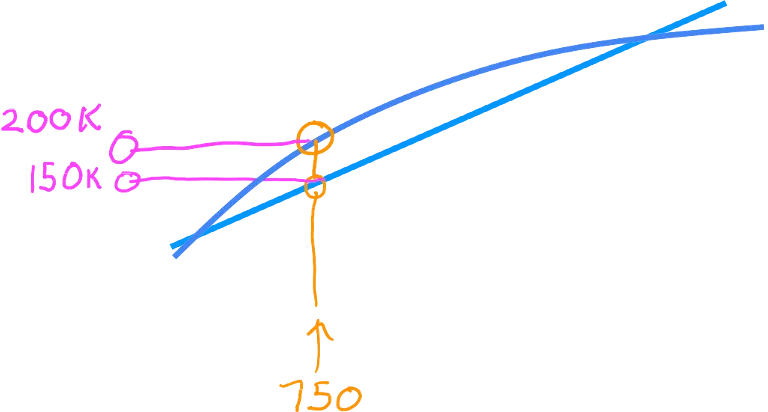
Regression

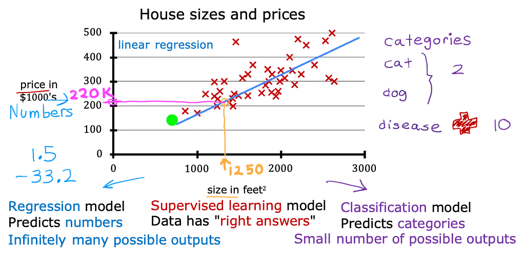
Predict a number with infinitely many possible outputs

stock price prediction (output: prices)
Test score prediction (output: final grade of the course)
Age prediction (input: face image, output: age)

Classification

Classification predicts categories with a small number of possible outputs

Email spam detection (spam/not spam) (binary classification)
Face shape classification
Breast cancer detection (benign, malignant type 2, malignant type 1)

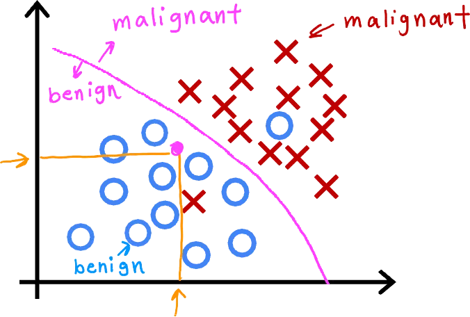
You can try mixing both tasks, e.g. using the regression to solve classification problems, but the results will depend upon your specific task and they are usually performing badly.

Unsupervised Learning

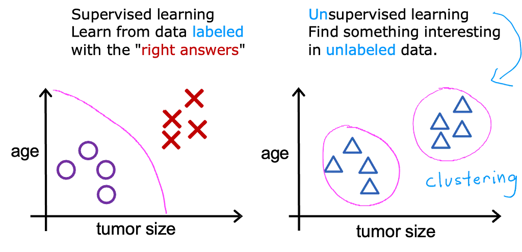
Unsupervised learning Find something interesting in unlabeled data.

No specific answers to the problem, clustering the data into n groups.

Terminology of Machine Learning

Dataset

Training set: Data used to train the model
Validation set: Data used to valid the model (validate during the training)
Testing set: Data used to test the model (test for the purpose data)

Cost Function

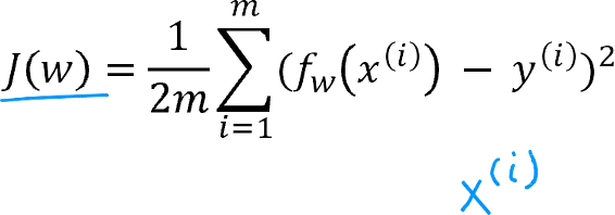
Cost (Loss): Difference between Target and Prediction
Cost Function: The method for distinguishing the Difference. E.g. MSE (Mean Square Error)

Objective

Model: selected method for solving the problem, sometimes called “Function”

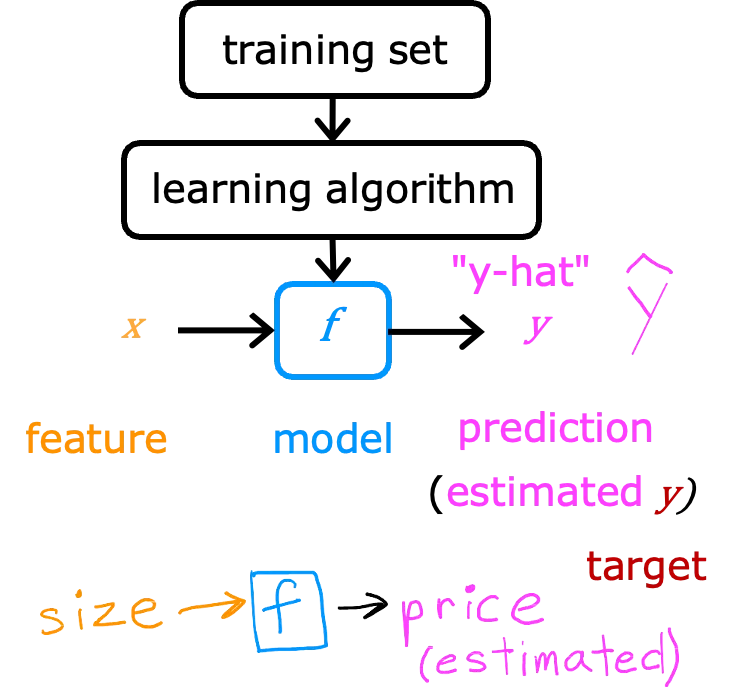
The procedure and terms of Machine Learning

Features (Input): x
Prediction (Output): estimated y or y-hat
Target (Supervised learning): y, so-called “Ground Truth”

Linear Regression

A basic Machine learning approach. It could be regression and classification, the difference is the output assumption.

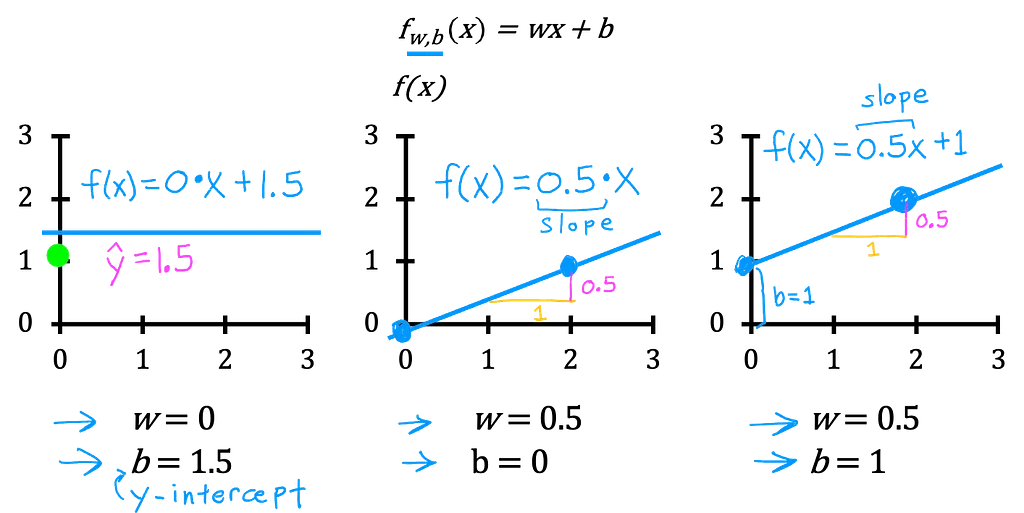
y = J(w, b)= w x + b

Simplified version

y = J(w)= w_1 x + w_0 1 = w x

Correction: The original writes the model as $J(w, b)$ ; more precisely, the model is $f_{w,b}(x) = wx + b$ and $J$ is the cost. For classification, logistic regression is used.

What do parameters (w, b) do?

Objective

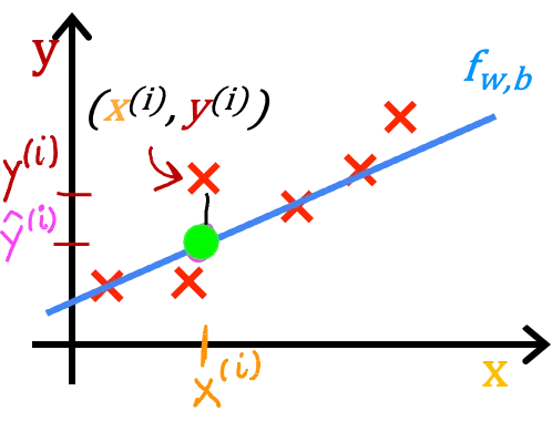
Minimize the difference (cost) between the prediction (y-hat) and the answer (y)

Find w, b:
y^(i) is close to y^(i) for all (x^(i) , y^(i)).

Correction: The original says “y^(i) is close to y^(i)”; more precisely, $\hat{y}^{(i)}$ is close to $y^{(i)}$ .

Cost Function

The formulas in text (2026 addition)

MSE cost over $m$ examples, and the update with learning rate $\alpha$ :

J(w,b) = \frac{1}{2m}\sum_{i=1}^{m}\left(f_{w,b}(x^{(i)}) - y^{(i)}\right)^2, \qquad w \leftarrow w - \alpha \frac{\partial J}{\partial w}

What is the best function we can get?

The Objective is the minimum point of the curve. Approaching to the minimum by changing parameters (w).

fixed x with different w

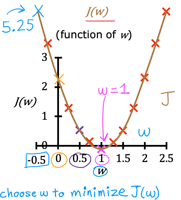
fixed x with different w

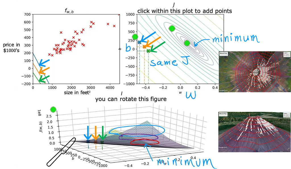
Gradient Decent

The purpose is to minimize the cost. However, the problems usually have multiple minimums (local minima and global minima). So, we will try our best to find out the lowest value of the local minimum which is close to the global minimum.

Gradient Descent is an optimization algorithm for finding a local minimum of a differentiable function. Gradient descent in machine learning is simply used to find the values of a function’s parameters (coefficients) that minimize a cost function as far as possible.

Wikipedia

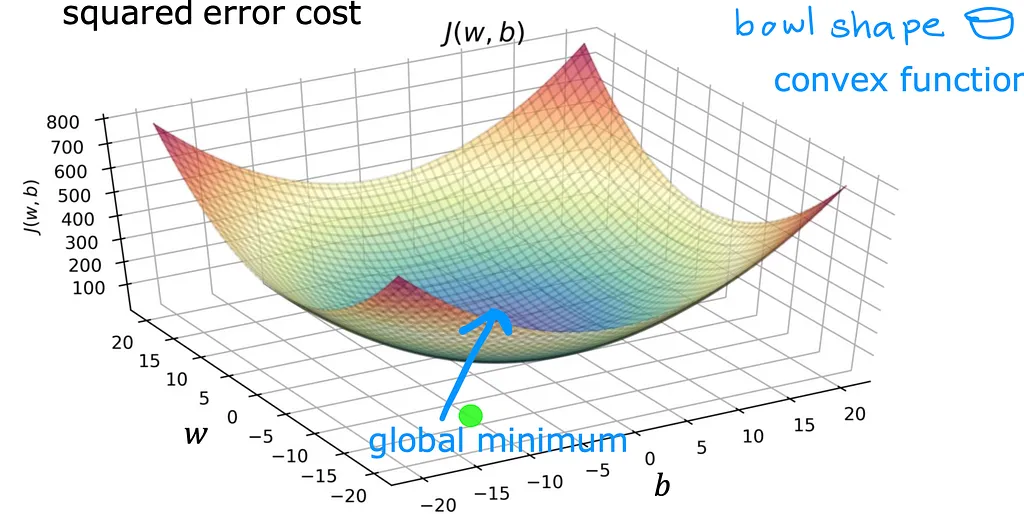
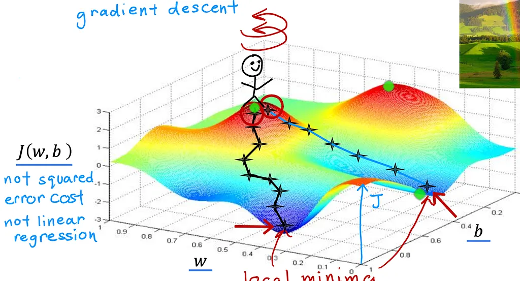
Algorithm

repeat the process until convergence

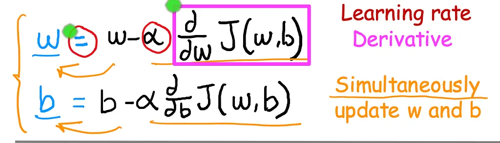
learning rate (alpha, or rho): , the step size of the optimization

Too Large

Overshoot, never reach minimum
Fail to converge, diverge

Too Small

Gradient descent may be slow

Cost = 0

The minimum points

Correction: The original says “Cost = 0” at the minimum; more precisely, the derivative is 0 there.

Derivative: the “direction” of the optimization steps

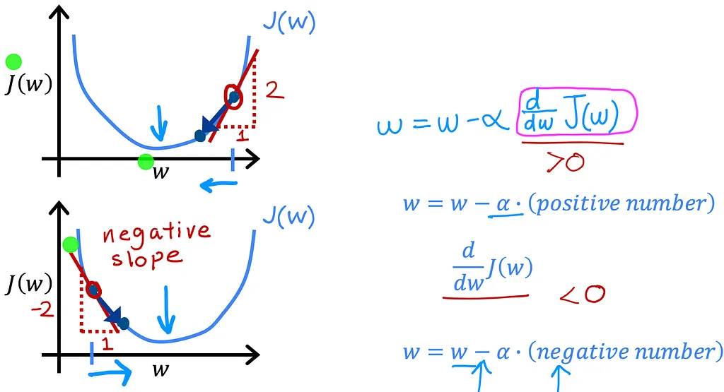
Optimal Process of Gradient Descent

Near a local minimum,

Derivative becomes smaller (By the nature of gradient descent)
Update steps become smaller (By some specific optimization methods)

Stochastic Gradient Descent (SGD)

The insight of stochastic gradient descent is that the gradient is an expectation. The expectation may be approximately estimated using a small set of samples.

For a fixed model size, the cost per GD update depends on the training set size m, and requires a huge amount of computational cost for training the large dataset.

For SGD, it uses part of the data (Batch) for each step (iteration).

Batch and mini-batch

Batch: Split the training set into n pieces
minibatch stochastic methods: Split the training set into pieces with minibatch size (or batch size) as n.

Correction: The original says “Batch” splits the training set into pieces; more precisely, batch gradient descent uses the whole set each step (though “batch size” in code means minibatch size).

References

Deep Learning

Slides from Machine Learning Specialization by Andrew Ng