Chapter 8 · Image Compression and Watermarking

What you’ll learn

• The three kinds of redundancy that compression removes, and how entropy puts a floor under lossless coding
• How the classic lossless coders work: Huffman, Golomb, arithmetic, LZW, run-length, symbol-based and bit-plane coding
• How JPEG turns an image into 8×8 DCT blocks, quantizes them, and why it shows blocks at low quality
• How predictive coding (DPCM, motion compensation) and wavelet coding (JPEG 2000) exploit neighboring pixels
• How to hide a watermark in the least significant bits or in DCT coefficients, and why one survives JPEG and the other does not
• Where learned (neural) codecs and deep-learning watermarks fit into this picture today

The big picture

A raw 512×512 color photo is 786,432 bytes. The same photo as a JPEG can be a few tens of kilobytes and still look fine. Compression is the art of finding out which bits are predictable or invisible, and then not storing them.

Nearly every image you see has been compressed, and many vision datasets are stored as JPEG, so models learn on images that already carry compression artifacts. Watermarking matters for ownership and, increasingly, for marking images made by generative models. Following the textbook [1], we cover fundamentals, then a toolbox of coding methods, then watermarking.

Fundamentals

In plain words: an image file usually contains more bits than the information it carries. Compression removes the extra bits; a good measure of “information” tells us how far we can go.

Compression ratio and redundancy

If an image takes $b$ bits uncompressed and $b'$ bits compressed, the compression ratio and relative data redundancy are

$$C = \frac{b}{b'}, \qquad R = 1 - \frac{1}{C}.$$

Here $C$ is a pure number (10 means “ten to one”) and $R$ is the fraction of the original data that was redundant. With $C = 10$, $R = 0.9$: 90% of the bits carried no new information.

Images contain three kinds of redundancy:

• Coding redundancy. A fixed 8-bit code spends 8 bits on every gray level, common or rare. Variable-length codes waste fewer bits.
• Spatial and temporal redundancy. Neighboring pixels, and consecutive video frames, are strongly correlated, so coding each pixel independently repeats information.
• Irrelevant information. Detail a viewer does not notice. Removing it is irreversible (lossy compression); removing only the first two kinds is lossless.

Measuring information: entropy

A symbol that occurs with probability $P(a)$ carries $I(a) = -\log_2 P(a)$ bits of information: rare events are surprising and carry more bits. Averaging over the source alphabet gives the entropy

$$H = -\sum_{j=1}^{J} P(a_j)\,\log_2 P(a_j) \quad \text{bits/symbol},$$

where $a_1, \dots, a_J$ are the possible symbols (for an 8-bit image, the 256 gray levels) and $P(a_j)$ is their probability. The noiseless source coding theorem says that no lossless code can use fewer than $H$ bits per symbol on average when symbols are coded one at a time and independently; good codes come close to $H$.

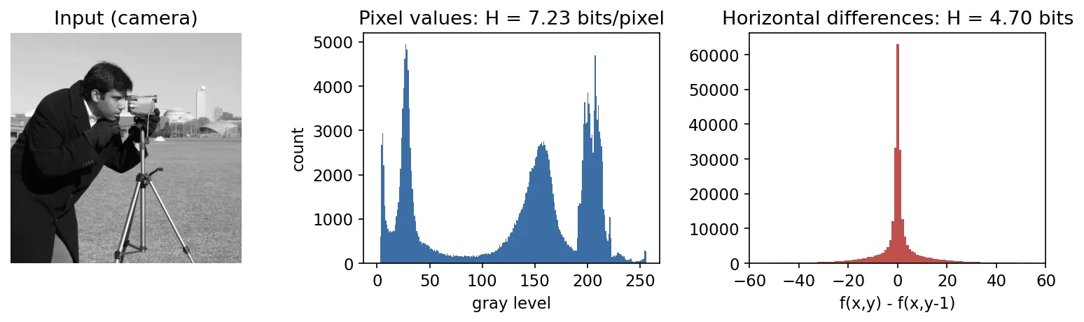
For a real image we only have estimates. The first-order estimate uses the normalized histogram $p_r(r_k) = n_k / MN$, where $n_k$ counts pixels with gray level $r_k$ in an $M \times N$ image. Figure 8.1 shows why the estimate depends on what you call a “symbol”. The camera image has a first-order entropy of 7.23 bits/pixel, barely below 8. If we instead code the difference between each pixel and its left neighbor, the entropy drops to 4.70 bits. The differences are not more clever; they simply remove the spatial redundancy that the histogram cannot see. This is the idea behind predictive coding later in the chapter.

import numpy as np
from skimage import data

def entropy(x):
    _, counts = np.unique(x, return_counts=True)
    p = counts / counts.sum()
    return -(p * np.log2(p)).sum()

img = data.camera()
print(f"H(pixels) = {entropy(img):.2f} bits")                          # 7.23
print(f"H(diffs)  = {entropy(np.diff(img.astype(int), axis=1)):.2f} bits")  # 4.70

Fidelity criteria

When compression is lossy we need to measure the damage. Let $f(x,y)$ be the original and $\hat f(x,y)$ the decompressed $M \times N$ image. The root-mean-square error and the peak signal-to-noise ratio are

$$e_{\text{rms}} = \sqrt{\frac{1}{MN}\sum_{x=0}^{M-1}\sum_{y=0}^{N-1}\big[\hat f(x,y) - f(x,y)\big]^2}, \qquad \text{PSNR} = 20\log_{10}\frac{L_{\max}}{e_{\text{rms}}}\ \text{dB},$$

where $L_{\max}$ is the largest possible pixel value (255 for 8-bit images). Higher PSNR means smaller error; as a rough guide, differences near 40 dB are hard to see and those below 25 dB are obvious, though this depends on content.

These objective criteria are easy to compute but do not always agree with people. Subjective criteria ask observers to rate images on a scale (from “excellent” to “unusable”) or to compare pairs.

Image compression models

Almost every codec in this chapter fits one block diagram. The encoder has three stages:

1. a mapper that transforms the image into a form with less redundancy (differences, transform coefficients, run lengths);
2. a quantizer that discards precision according to a fidelity target (this is the only lossy stage, and lossless codecs omit it);
3. a symbol coder that assigns short codes to frequent symbols (Huffman, arithmetic, Golomb…).

The decoder runs a symbol decoder and an inverse mapper. There is no “inverse quantizer” that can bring back lost precision.

Formats, containers and standards

A file format fixes how bits are laid out, a container wraps coded images plus metadata (and can hold different codecs), and a compression standard defines the coding method. The common ones:

Name	Type	Core method	Lossless?
JPEG (ISO/IEC 10918-1, ITU-T T.81) [2]	standard + format	8×8 DCT, quantization, Huffman or arithmetic coding	lossy (baseline)
JPEG 2000 (ISO/IEC 15444) [3]	standard + format	discrete wavelet transform, bit-plane arithmetic coding	both
PNG [4]	format	per-row prediction filters + deflate (an LZ77 derivative)	lossless
JPEG-LS [10]	standard	context-based prediction + Golomb-type codes	lossless / near-lossless
JPEG XL (ISO/IEC 18181) [5]	standard + format	lossy and lossless modes; lossless transcoding of JPEG files	both
HEIF (ISO/IEC 23008-12) [7]	container	holds HEVC-coded images (.heic), among others	depends on codec
AVIF [6]	HEIF-based format	AV1 intra-frame coding stored in HEIF	both

Huffman coding

In plain words: give the most common symbols the shortest codewords, and build the code so no codeword is the beginning of another, so the bit stream can be read without separators.

Huffman’s algorithm [8] builds an optimal prefix code for a known set of symbol probabilities, when symbols are coded one at a time. It works bottom-up:

1. List the symbols with their probabilities.
2. Merge the two least probable entries into a new node whose probability is their sum.
3. Repeat until one node (probability 1) remains.
4. Walk from the root to each leaf, writing 0 for one branch and 1 for the other. The path is the codeword.

A worked example

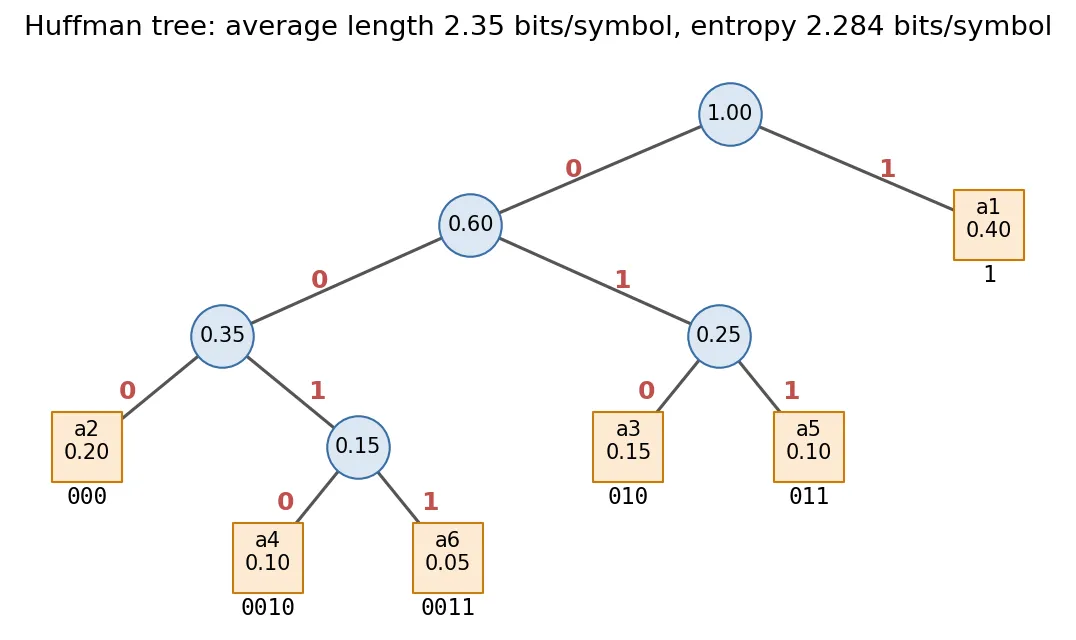
Take a source with six symbols: $P(a_1) = 0.40$, $P(a_2) = 0.20$, $P(a_3) = 0.15$, $P(a_4) = 0.10$, $P(a_5) = 0.10$, $P(a_6) = 0.05$. The merges are:

Step	Merge	New node
1	$a_6$ (0.05) + $a_4$ (0.10)	0.15
2	$a_5$ (0.10) + $a_3$ (0.15)	0.25
3	$a_2$ (0.20) + node 0.15	0.35
4	node 0.25 + node 0.35	0.60
5	$a_1$ (0.40) + node 0.60	1.00

The tree in Figure 8.2 gives $a_1 =$ 1, $a_2 =$ 000, $a_3 =$ 010, $a_4 =$ 0010, $a_5 =$ 011, $a_6 =$ 0011. The average codeword length is

$$L_{\text{avg}} = \sum_j P(a_j)\, l(a_j) = 0.4(1) + 0.2(3) + 0.15(3) + 0.1(4) + 0.1(3) + 0.05(4) = 2.35 \ \text{bits/symbol},$$

where $l(a_j)$ is the length of the codeword for $a_j$. A fixed-length code needs 3 bits and the entropy is $H = 2.284$ bits, so Huffman is within 3% of the bound. Ties can be broken either way; other choices change the codewords but not the average length.

Decoding is a walk down the tree: read bits until you hit a leaf, output its symbol, return to the root. Because no codeword is a prefix of another, the code is instantaneous and uniquely decodable. JPEG uses Huffman tables for its quantized coefficients [2].

import heapq, itertools

def huffman_codes(probs):
    tick = itertools.count()                       # tie-breaker for equal probabilities
    heap = [(p, next(tick), {s: ""}) for s, p in probs.items()]
    heapq.heapify(heap)
    while len(heap) > 1:
        p1, _, c1 = heapq.heappop(heap)            # least probable
        p2, _, c2 = heapq.heappop(heap)            # second least
        merged = {s: "1" + c for s, c in c1.items()}
        merged |= {s: "0" + c for s, c in c2.items()}
        heapq.heappush(heap, (p1 + p2, next(tick), merged))
    return heap[0][2]

P = {"a1": .40, "a2": .20, "a3": .15, "a4": .10, "a5": .10, "a6": .05}
print(huffman_codes(P))   # a1:'1', a2:'000', a3:'010', a4:'0010', a5:'011', a6:'0011'

The limitation: every symbol costs at least one whole bit. When one symbol has probability 0.95, its information is only 0.07 bits, but Huffman still spends 1 bit on it. Arithmetic coding, below, removes that limit.

Golomb coding

In plain words: when small numbers are common and big numbers are rare, write a number as “how many full groups of $m$” (in tally marks) plus “what is left over” (in ordinary binary).

Golomb codes [9] are designed for nonnegative integers $n$ with a geometric-like distribution, which is exactly what prediction residuals look like after mapping. For a parameter $m > 0$, the code $G_m(n)$ is the concatenation of

1. the unary code of the quotient $q = \lfloor n/m \rfloor$: $q$ ones followed by a zero;
2. the truncated binary code of the remainder $r = n \bmod m$: with $k = \lceil \log_2 m \rceil$ and $c = 2^k - m$, values $r \lt c$ use $k-1$ bits, and the rest are coded as $r + c$ in $k$ bits.

$n$	0	1	2	3	4	5	6	7	8
$G_4(n)$	000	001	010	011	1000	1001	1010	1011	11000
$G_3(n)$	00	010	011	100	1010	1011	1100	11010	11011

When $m$ is a power of two, the remainder is just the low $k$ bits of $n$, so encoding needs only shifts and masks. Prediction residuals $e$ are signed, so a codec first maps them to nonnegative integers, for example $M(e) = 2e$ for $e \ge 0$ and $M(e) = 2|e| - 1$ for $e \lt 0$, which interleaves $0, -1, 1, -2, 2, \dots$. JPEG-LS [10] combines this mapping with Golomb codes whose power-of-two parameter is adapted to local context.

import numpy as np

def golomb(n, m):
    q, r = divmod(n, m)
    unary = "1" * q + "0"
    k = int(np.ceil(np.log2(m)))
    c = 2**k - m                        # how many remainders get k-1 bits
    if r < c:
        tail = format(r, f"0{k-1}b") if k > 1 else ""
    else:
        tail = format(r + c, f"0{k}b")
    return unary + tail

print([golomb(n, 3) for n in range(9)])

Arithmetic coding

In plain words: instead of giving each symbol its own codeword, describe the whole message as one very precise number between 0 and 1.

Arithmetic coding [11] starts from the interval $[0, 1)$. For each symbol, it shrinks the current interval to the sub-interval that the symbol owns, in proportion to its probability. After the message, any number inside the final interval identifies the message. If the current interval is $[\ell, h)$ and the next symbol $s$ owns the cumulative range $[F_{\text{lo}}(s), F_{\text{hi}}(s))$, then

$$\ell' = \ell + (h - \ell)\,F_{\text{lo}}(s), \qquad h' = \ell + (h - \ell)\,F_{\text{hi}}(s).$$

The final width equals the product of the symbol probabilities, so the number of bits needed is about $-\log_2 \prod_i P(s_i) = \sum_i -\log_2 P(s_i)$, which is exactly the information content of the message. There is no “one bit per symbol” floor.

Worked example

Let $P(a) = 0.6$, $P(b) = 0.3$, $P(c) = 0.1$, so $a$ owns $[0, 0.6)$, $b$ owns $[0.6, 0.9)$ and $c$ owns $[0.9, 1)$. Encode the message abac:

After	Interval
a	$[0, 0.6)$
b	$[0.36, 0.54)$
a	$[0.36, 0.468)$
c	$[0.4572, 0.468)$

The width is $0.6 \times 0.3 \times 0.6 \times 0.1 = 0.0108$, or $-\log_2 0.0108 \approx 6.5$ bits of information. The 7-bit binary fraction $0.0111011_2 = 0.4609375$ falls inside the interval, so 7 bits identify the message (plus a way to signal its end, such as a length or an end-of-message symbol).

Real coders use integer arithmetic with renormalization so that the interval never underflows, and they usually use adaptive probability models that are updated as symbols arrive, so no table needs to be sent. JPEG 2000’s coefficient coder feeds an adaptive binary arithmetic coder [14], and the learned codecs in the Modern view section also end with arithmetic coding.

LZW coding

In plain words: build a dictionary of phrases as you go; whenever a phrase repeats, send its dictionary index instead of spelling it out.

The Lempel–Ziv–Welch (LZW) algorithm [12] starts with a dictionary holding all single symbols (codes 0–255 for 8-bit pixels). It reads the input, growing the current phrase $w$ while $w$ followed by the next symbol is still in the dictionary. When it is not, the coder outputs the code for $w$, adds the extended phrase as a new entry (256, 257, …), and restarts from the new symbol. The decoder rebuilds the same dictionary from the codes it receives, so no dictionary is transmitted.

For a row that alternates 39 39 126 126 four times (16 pixels), the output is ten codes:

def lzw_encode(seq):
    table = {(v,): v for v in range(256)}
    w, out = (), []
    for x in seq:
        wx = w + (x,)
        if wx in table:
            w = wx
        else:
            out.append(table[w])
            table[wx] = len(table)
            w = (x,)
    if w:
        out.append(table[w])
    return out

row = [39, 39, 126, 126] * 4
print(lzw_encode(row))   # [39, 39, 126, 126, 256, 258, 260, 259, 257, 126]

Codes 256 onward stand for 39 39, 39 126, 126 126, 126 39, 39 39 126, and so on. The longer the repetition, the longer the phrases and the better the ratio. LZW needs no prior knowledge of the probabilities, which made it popular in general-purpose file formats. PNG uses the related LZ77-style deflate method [4].

Run-length coding

In plain words: “0000 11 00000 1” becomes “four 0s, two 1s, five 0s, one 1”.

Run-length encoding (RLE) replaces each run of identical values with a pair (value, length). For binary images only the lengths are needed, if the first run’s color is agreed on. The run lengths themselves are then coded with a variable-length code, since short runs are more frequent than long ones.

import numpy as np

def rle(row):
    starts = np.r_[0, np.flatnonzero(np.diff(row)) + 1]
    lengths = np.diff(np.r_[starts, len(row)])
    return list(zip(row[starts].tolist(), lengths.tolist()))

print(rle(np.array([0, 0, 0, 0, 1, 1, 0, 0, 0, 0, 0, 1])))  # [(0, 4), (1, 2), (0, 5), (1, 1)]

RLE works well for documents, line drawings and bit planes, and poorly for noisy photographs where runs are short. Two-dimensional variants code the positions of color transitions in the current row relative to the transitions in the row above, which exploits vertical correlation too. JPEG uses a form of run-length coding for the many zero-valued coefficients produced by quantization [13].

Symbol-based coding

In plain words: a scanned page is mostly the same few letters again and again. Store each letter shape once, then just say “letter 7 goes here”.

In symbol-based (token-based) coding, frequently occurring sub-images, called symbols, are stored once in a symbol dictionary. The image becomes a list of triplets $(x_i, y_i, t_i)$: the position of each occurrence and the index $t_i$ of its dictionary entry. A text page with thousands of characters but about a hundred distinct glyph shapes compresses very well, since each occurrence costs two coordinates and an index, which are then entropy-coded.

If an occurrence may match an entry that is only similar, the method becomes lossy. That improves the ratio, but a careless matcher can substitute a wrong character, such as two digits that look alike in a low-resolution scan. Safe systems keep the match threshold conservative, or also code the residual between occurrence and token to stay lossless.

Bit-plane coding

In plain words: split an 8-bit image into eight black-and-white pictures, one per bit, and compress each with a binary method.

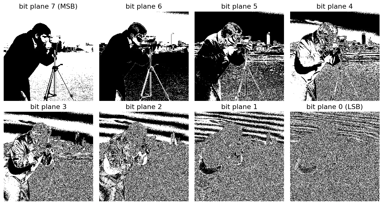
A gray level $a = a_7 2^7 + a_6 2^6 + \dots + a_0 2^0$ has eight bits $a_7, \dots, a_0$. Collecting bit $k$ of every pixel gives bit plane $k$ (Figure 8.3). The high-order planes look like coarse versions of the picture and contain large uniform areas; the low-order planes look like noise. Each plane can be coded with run-length or other binary methods.

A weakness of the plain binary code is that a small change in gray level can flip many bits: 127 is 01111111 and 128 is 10000000. The Gray code fixes this by making consecutive values differ in exactly one bit:

$$g_7 = a_7, \qquad g_i = a_i \oplus a_{i+1}, \quad 0 \le i \le 6,$$

where $\oplus$ is exclusive OR. With Gray-coded planes, smooth areas produce longer runs. On the camera image, bit plane 6 changes value between horizontal neighbors 6.4% of the time; its Gray-coded counterpart changes only 3.2% of the time, so its runs are about twice as long on average. In NumPy the conversion is one line: gray = img ^ (img >> 1).

JPEG 2000 also codes its wavelet coefficients bit plane by bit plane, from the most significant down, which is what makes its bit stream truncatable at any rate [14].

Block transform coding

In plain words: cut the image into small tiles, describe each tile as a mix of standard patterns (smooth to busy), keep the important patterns, and throw away the fine ones the eye barely notices.

A block transform coder splits the image into non-overlapping $n \times n$ subimages, transforms each one, quantizes the coefficients, and entropy-codes the result. The transform does not compress by itself; it packs most of the energy into a few coefficients so that the rest can be quantized coarsely or dropped.

Transform selection

For an $n \times n$ block $g(x,y)$, the 2-D discrete cosine transform (DCT) is

$$T(u,v) = \alpha(u)\alpha(v)\sum_{x=0}^{n-1}\sum_{y=0}^{n-1} g(x,y)\cos\frac{(2x+1)u\pi}{2n}\cos\frac{(2y+1)v\pi}{2n},$$

with $\alpha(0) = \sqrt{1/n}$ and $\alpha(u) = \sqrt{2/n}$ for $u = 1, \dots, n-1$; $u, v$ index the horizontal and vertical frequencies. The Karhunen–Loève transform (KLT, Chapter 7) packs energy best in the mean-square sense, but its basis depends on the data and must be computed and sent. The DCT is fixed, has fast algorithms, and for highly correlated images its basis is close to the KLT’s. It also beats the DFT for blocks: the DFT treats a block as periodic, so the jump between its left and right edges creates spurious high frequencies, while the DCT’s implied even symmetric extension has no such jump.

Subimage size

Larger blocks capture more correlation and pack energy better, but cost more computation, and an error spreads over a larger area. Gains level off quickly beyond about $8 \times 8$ or $16 \times 16$. JPEG chose a fixed $8 \times 8$; many newer codecs choose among several block sizes, using large blocks in smooth regions and small ones around detail.

Bit allocation

After the transform, we decide how many bits each coefficient gets.

• Zonal coding keeps a fixed zone of coefficients (usually the low frequencies, which have the largest variance across blocks) in every block.
• Threshold coding keeps whichever coefficients exceed a threshold in each block, so the kept set adapts to content.

The common practical form of threshold coding divides each coefficient by an entry of a normalization (quantization) array $Z$ and rounds:

$$\hat T(u,v) = \operatorname{round}\!\left[\frac{T(u,v)}{Z(u,v)}\right],$$

where $\hat T(u,v)$ is the integer that is actually coded. The decoder multiplies back, $\dot T(u,v) = \hat T(u,v)\,Z(u,v)$, and inverts the DCT. Large entries of $Z$ at high frequencies throw away fine detail; small entries at low frequencies keep the coarse structure.

JPEG baseline

The JPEG baseline coder for 8-bit grayscale [2][13] does exactly this:

1. Shift pixel values by $-128$ so they are centered on zero.
2. Compute the $8 \times 8$ DCT of each block.
3. Quantize with a $Z$ table. The standard gives an example luminance table; a widely used convention scales it by a quality factor $q \in [1, 100]$, with scale $s = 5000/q$ for $q \lt 50$ and $s = 200 - 2q$ otherwise (in percent).
4. Code the DC coefficient $\hat T(0,0)$ as the difference from the previous block’s DC.
5. Reorder the 63 AC coefficients in a zigzag from low to high frequency, so zeros cluster at the end, and code them as (run of zeros, nonzero value) pairs with Huffman tables, ending each block with an end-of-block symbol.

Figure 8.4 follows one dark, smooth block through steps 2–3 at $q = 50$. It has a large DC term ($-603$, because of the level shift) and a few low-frequency terms. After quantization only 6 of 64 integers are nonzero, yet the reconstruction is off by only a few gray levels.

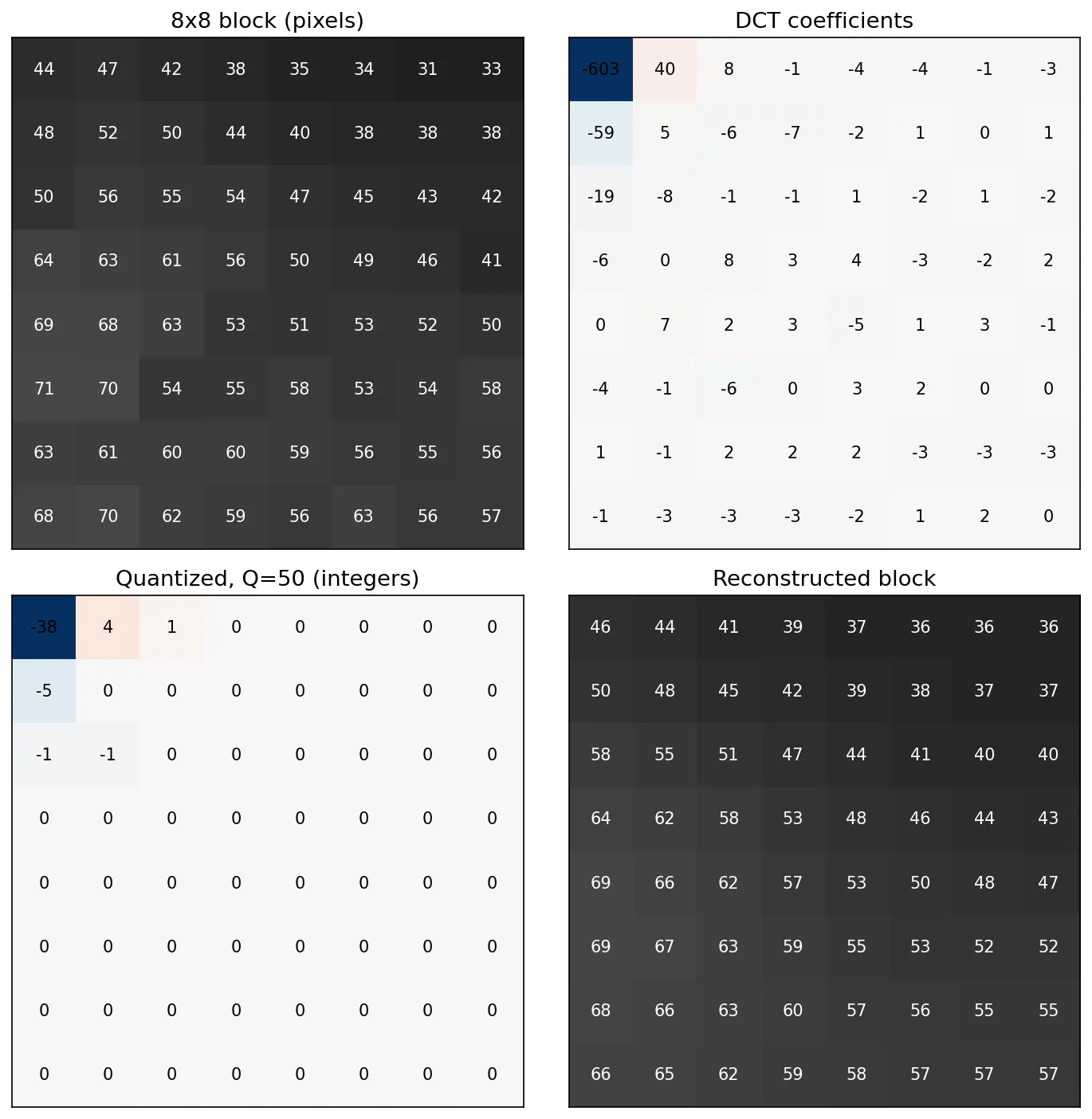
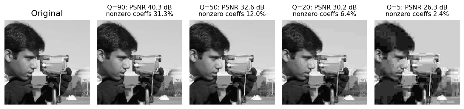
Figure 8.5 applies the same pipeline (without the entropy coder) to the whole image at four quality settings. PSNR drops from 40.3 dB at $q = 90$ to 26.3 dB at $q = 5$, while the fraction of nonzero coefficients falls from 31.3% to 2.4%. At low quality the familiar artifacts appear: blocking (visible 8×8 seams, because each block is coded independently) and ringing near edges (because the high frequencies that make a sharp edge were removed).

import numpy as np
from scipy.fft import dctn, idctn

Q50 = np.array([[16,11,10,16,24,40,51,61],[12,12,14,19,26,58,60,55],
                [14,13,16,24,40,57,69,56],[14,17,22,29,51,87,80,62],
                [18,22,37,56,68,109,103,77],[24,35,55,64,81,104,113,92],
                [49,64,78,87,103,121,120,101],[72,92,95,98,112,100,103,99]])

def dct_codec(img, Q):
    f = img.astype(float) - 128                       # level shift
    H, W = f.shape
    B = f.reshape(H//8, 8, W//8, 8).swapaxes(1, 2)   # (H/8, W/8, 8, 8) blocks
    q = np.round(dctn(B, axes=(2, 3), norm="ortho") / Q)
    rec = idctn(q * Q, axes=(2, 3), norm="ortho")
    rec = rec.swapaxes(1, 2).reshape(H, W) + 128
    return np.clip(rec.round(), 0, 255).astype(np.uint8), q

rec, q = dct_codec(img, Q50)     # PSNR 32.6 dB, 12.0% nonzero coefficients

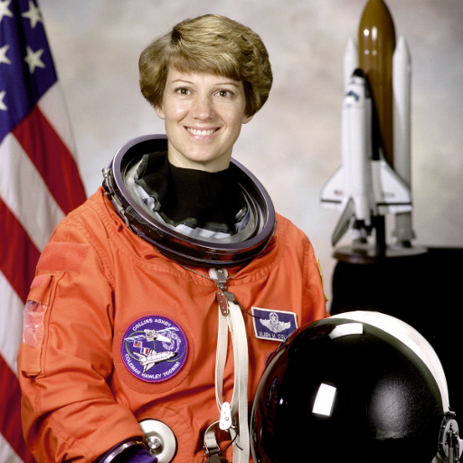
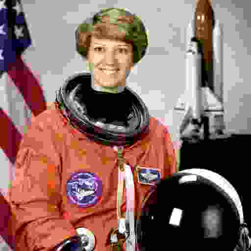
Drag the slider below to compare a lossless PNG of a color test image (465 kB) with a real JPEG at quality 4 (7.6 kB, about 60 times smaller). Look at the flat background, the face and the color edges: blocks, ringing and color bleeding (the color channels are stored at lower resolution and quantized harder) are all visible.

Original (PNG)JPEG q=4

Predictive coding

In plain words: guess each pixel from the ones you have already sent, and only send how wrong the guess was. Good guesses mean small numbers, and small numbers are cheap.

Lossless predictive coding

The encoder forms a prediction $\hat f(n)$ of pixel $f(n)$ from previously coded pixels and codes the prediction error

$$e(n) = f(n) - \hat f(n), \qquad \hat f(n) = \operatorname{round}\!\left[\sum_{i=1}^{m}\alpha_i f(n-i)\right],$$

where $m$ is the predictor order and $\alpha_i$ are the prediction coefficients. The decoder computes the same prediction and adds $e(n)$ back, so the reconstruction is exact. Figure 8.1 already showed the payoff: the simplest predictor, “same as the left neighbor”, lowers the entropy from 7.23 to 4.70 bits/pixel.

PNG lets each row choose among five filters: none, left (Sub), above (Up), the average of left and above, and the Paeth predictor [4]. JPEG-LS [10] uses the median edge detector: with $a$ the left, $b$ the upper and $c$ the upper-left neighbor,

$$\hat f = \begin{cases} \min(a,b) & c \ge \max(a,b) \\ \max(a,b) & c \le \min(a,b) \\ a + b - c & \text{otherwise.} \end{cases}$$

The first two cases pick the neighbor on the correct side of a horizontal or vertical edge; the third assumes a smooth plane.

Motion compensation

Video adds a time axis. Instead of predicting from neighbors in the same frame, a motion-compensated predictor copies a block from a previously decoded frame, displaced by a motion vector $(d_x, d_y)$ found by searching for the best match (for example, the smallest sum of absolute differences). The encoder sends the motion vector and the residual, usually transform-coded as in the previous section. Frames coded only from themselves (intra frames) provide entry points for random access; predicted frames are much smaller. HEVC, whose still-image form is stored in HEIC files [7], and AV1, used by AVIF [6], both combine this kind of inter-frame prediction with transform coding.

Lossy predictive coding (DPCM)

If we quantize the prediction error, $\dot e(n) = Q[e(n)]$, we get differential pulse-code modulation (DPCM). The key detail is that the encoder must predict from the reconstructed values $\dot f(n) = \dot e(n) + \hat f(n)$, the same values the decoder will have. If the encoder predicted from the originals instead, quantization errors would accumulate in the decoder (drift).

import numpy as np

def dpcm(row, step):
    """Lossy DPCM with previous-sample prediction and a uniform quantizer."""
    rec = np.empty(len(row)); prev = 128.0; idx = []
    for i, x in enumerate(row.astype(float)):
        e = x - prev                       # prediction error
        k = int(np.round(e / step))        # quantizer index: this is what is sent
        prev = prev + k * step             # reconstruction, identical in the decoder
        rec[i] = prev; idx.append(k)
    return np.array(idx), rec

On one row of the camera image with step 8, the indices have an entropy of 1.87 bits/sample and the reconstruction has a PSNR of 40.8 dB. With a very coarse quantizer, two typical distortions appear: slope overload (the reconstruction cannot climb fast enough at a steep edge) and granular noise (it jitters in flat areas).

Optimal predictors and quantizers

The optimal linear predictor chooses $\alpha_1, \dots, \alpha_m$ to minimize the mean-square prediction error $E\{e^2(n)\}$. Setting the derivatives to zero gives the normal equations

$$\mathbf R\,\boldsymbol\alpha = \mathbf r, \qquad \boldsymbol\alpha = \mathbf R^{-1}\mathbf r,$$

where $\mathbf R$ is the $m \times m$ autocorrelation matrix with entries $E\{f(n-i)f(n-j)\}$ and $\mathbf r$ is the vector with entries $E\{f(n)f(n-i)\}$. (The analysis usually ignores the quantizer inside the loop, which is accurate when quantization is fine.)

The optimal quantizer for a given number of levels minimizes the mean-square quantization error for the error distribution. Two conditions characterize it: each decision boundary lies halfway between its two neighboring reconstruction levels, and each reconstruction level is the centroid (conditional mean) of the probability mass in its interval. Because prediction errors are peaked at zero, the optimal levels are dense near zero and sparse in the tails. In practice, a uniform quantizer followed by a variable-length code is nearly as good and much simpler.

Wavelet coding

In plain words: instead of chopping the image into tiles, split it into a blurry small version plus layers of detail at different scales. Most detail values are near zero, so they are cheap to store, and there are no tile seams.

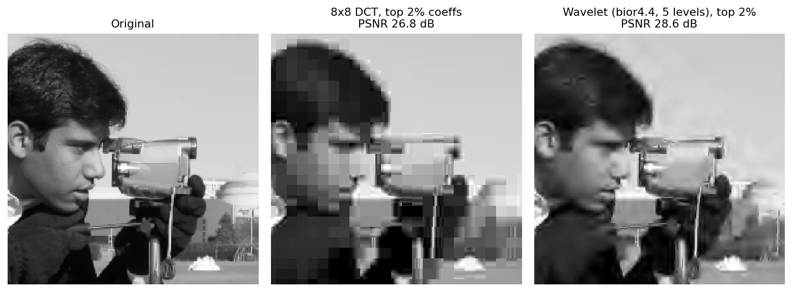
A wavelet coder applies the discrete wavelet transform of Chapter 7, quantizes the coefficients, and entropy-codes them. Because the basis functions overlap and are localized at many scales, a wavelet coder has no block boundaries and degrades by blurring and mild ringing rather than by blocking. Figure 8.6 compares an 8×8 DCT and a five-level wavelet transform that each keep the same 2% of their coefficients (the largest in magnitude). The DCT result is a mosaic at 26.8 dB; the wavelet result is smoother and reaches 28.6 dB.

import numpy as np, pywt

def wavelet_code(img, keep=0.02, wavelet="bior4.4", level=5):
    c = pywt.wavedec2(img.astype(float), wavelet, level=level, mode="periodization")
    arr, slices = pywt.coeffs_to_array(c)
    t = np.quantile(np.abs(arr), 1 - keep)            # keep the largest 2%
    arr[np.abs(arr) < t] = 0
    c = pywt.array_to_coeffs(arr, slices, output_format="wavedec2")
    return np.clip(pywt.waverec2(c, wavelet, mode="periodization"), 0, 255)

This toy counts coefficients, not bits. A real coder must also signal which coefficients survived, which is where clever significance coding earns its keep.

Wavelet selection

The wavelet determines how well energy is packed and what artifacts look like. Image coders favor biorthogonal wavelets because they can be symmetric (so edges are not shifted) and have short filters. JPEG 2000 specifies two: an irreversible 9/7-tap filter pair for lossy coding and a reversible integer 5/3 filter pair for lossless coding [14]. PyWavelets’ bior4.4 used above has the same 9- and 7-tap lengths.

Decomposition level

Each level splits the current approximation into four half-size subbands. More levels make the representation sparser, but gains shrink after about five levels for typical image sizes, and quantizing very coarse coefficients affects large areas.

Quantizer design

Wavelet coders usually use a uniform scalar quantizer with an enlarged dead zone around zero:

$$q_b = \operatorname{sign}(c_b)\left\lfloor \frac{|c_b|}{\Delta_b} \right\rfloor,$$

where $c_b$ is a coefficient in subband $b$, $\Delta_b$ is that subband’s step size and $q_b$ the integer index. Small coefficients, most of which are noise, fall into the zero bin. Step sizes are chosen per subband, coarser for the high-frequency subbands where errors are less visible.

JPEG 2000

JPEG 2000 [3][14] builds a full system around these pieces. The image can be split into large tiles, color components are decorrelated with a component transform, and each tile is wavelet transformed and dead-zone quantized. Each subband is divided into small code blocks that are coded independently bit plane by bit plane with an adaptive arithmetic coder. Finally, the coded pieces are arranged into quality layers, so a single file can be decoded at lower resolution or lower quality just by reading a prefix of the stream. It also supports lossless coding and regions of interest coded at higher quality.

Digital image watermarking

In plain words: a watermark is extra information hidden in an image, like a signature, an owner ID or a “this was generated by a model” flag, that travels with the picture.

Kinds of watermarks

• Visible watermarks are overlays (a semi-transparent logo); they degrade the image and can often be cropped or painted out. Invisible watermarks stay below the visibility threshold and are recovered by a detector.
• A robust watermark survives compression, resizing, filtering and cropping (for ownership and provenance). A fragile one breaks under any change (for authentication). Semi-fragile marks survive mild compression but not content edits.
• Private (non-blind) detection needs the original image; blind detection does not.

Every scheme trades off imperceptibility (how little the image changes), robustness, capacity (how many bits are hidden) and security (whether someone without the key can find, remove or forge the mark).

A fragile example: least significant bits

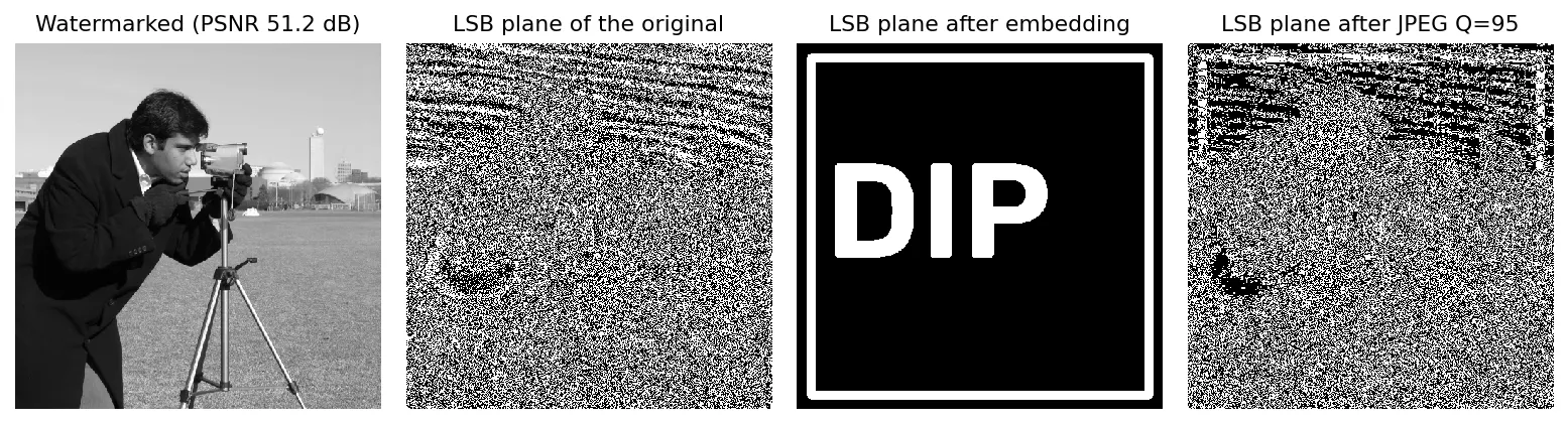
The simplest invisible watermark replaces the least significant bit (LSB) of each pixel with a bit of the mark: $f_w = 2\lfloor f/2 \rfloor + w$, with $w \in \{0, 1\}$. The change is at most one gray level, so the PSNR is about 51 dB.

def lsb_embed(cover, mark):          # cover: uint8 image, mark: 0/1 array of the same shape
    return (cover & 0xFE) | mark

def lsb_extract(img):
    return img & 1

Figure 8.7 embeds a binary “DIP” logo. Extraction is perfect from the PNG. After a single JPEG compression at quality 95, which looks identical to the eye, only 55% of the extracted bits match the mark, barely better than a coin flip. The LSB plane is the noise-like part of the image that every lossy coder discards first. That makes LSB marks useless for ownership but suitable as a fragile integrity check.

A robust example: DCT-domain watermark

To survive JPEG, hide the mark where JPEG keeps information: in low- to mid-frequency DCT coefficients. The scheme below is a simple one of our own. In each 8×8 block it compares two mid-frequency coefficients, $C(2,3)$ and $C(3,2)$, which JPEG quantizes with similar step sizes. To embed bit 1, it makes $C(2,3)$ exceed $C(3,2)$ by at least a margin $\alpha$; to embed bit 0, the reverse. The detector only checks which coefficient is larger, so it is blind.

import numpy as np
from scipy.fft import dctn, idctn

def blocks(img):
    H, W = img.shape
    return img.astype(float).reshape(H//8, 8, W//8, 8).swapaxes(1, 2).reshape(-1, 8, 8)

def unblocks(B, H, W):
    return B.reshape(H//8, W//8, 8, 8).swapaxes(1, 2).reshape(H, W)

def dct_embed(img, bits, alpha=12.0):
    C = dctn(blocks(img), axes=(1, 2), norm="ortho")
    for i, b in enumerate(bits):               # one bit per 8x8 block
        x, y = C[i, 2, 3], C[i, 3, 2]
        if (x - y if b else y - x) < alpha:    # enforce the order with margin alpha
            m = (x + y) / 2
            s = alpha / 2 if b else -alpha / 2
            C[i, 2, 3], C[i, 3, 2] = m + s, m - s
    out = unblocks(idctn(C, axes=(1, 2), norm="ortho"), *img.shape)
    return np.clip(out.round(), 0, 255).astype(np.uint8)

def dct_extract(img):
    C = dctn(blocks(img), axes=(1, 2), norm="ortho")
    return (C[:, 2, 3] > C[:, 3, 2]).astype(int)

On the 512×512 camera image this hides 4,096 bits (one per block). The margin $\alpha$ is the robustness dial:

Margin $\alpha$	PSNR of marked image	Bit errors after JPEG q=90	q=75	q=50
12	43.2 dB	0.10%	0.56%	36.6%
30	38.4 dB	0%	0%	0.05%

A small margin is nearly invisible but breaks once the JPEG step size at those positions exceeds the margin. A larger margin survives quality 50 at the cost of about 5 dB PSNR. Real systems add error-correcting codes, spread each bit over many blocks with a secret key, and adapt the strength to local texture, since the eye tolerates larger changes in busy regions.

Modern view

The classical pipeline (transform, quantize, entropy code) still underlies every deployed image codec. What has changed since about 2016 is that each stage can be learned, and that the same idea of trained encoders and decoders has reshaped watermarking.

Surveys worth reading

• Wallace (1992) [13] remains the clearest overview of JPEG’s design: the DCT, quantization tables, zigzag ordering, and the Huffman and arithmetic options. It is the right companion to the block transform section.
• Skodras, Christopoulos and Ebrahimi (2001) [14] is a tutorial review of JPEG 2000: tiling, the 9/7 and 5/3 wavelets, dead-zone quantization, code-block bit-plane coding and rate control. Its main takeaway is that JPEG 2000’s value lies less in raw efficiency than in features: scalability, region-of-interest coding and lossless operation in one bit stream.
• Hu, Yang, Ma and Liu (2021) [16] survey end-to-end learned lossy image compression along three axes, network architecture, entropy model and rate control, trace the milestones of each, and benchmark representative methods on CPU and GPU. Their own contribution, a coarse-to-fine hyperprior, illustrates the survey’s central theme: much of the progress lies in how well the entropy model predicts the latent representation.
• Yang, Mandt and Theis (2023) [17] is a monograph-length introduction to neural compression for a machine-learning audience. It reviews the information theory (entropy coding, rate-distortion theory) and the image-quality and perceptual metrics you need, then guides the reader through codecs built on normalizing flows, variational autoencoders, diffusion models and GANs.
• Zhong, Das, Alrasheedi and Tanvir (2023) [18] survey deep-learning image watermarking and sort methods into three families: jointly trained embedder–extractor networks, networks used as feature transforms around a classical embedding rule, and hybrids.

Learned image compression

Ballé et al. [15] replaced the DCT with a learned nonlinear analysis transform (a convolutional network) that maps the image $x$ to a latent $y$, which is quantized to $\hat y$ and decoded by a learned synthesis transform. The whole system is trained to minimize a rate-distortion loss

$$\mathcal L = R + \lambda D = E\left[-\log_2 p(\hat y)\right] + \lambda\, E\left[d(x, \hat x)\right],$$

where $R$ is the expected code length under the entropy model $p$, $D$ is a distortion such as MSE, and $\lambda$ sets the trade-off. Their key contribution was the scale hyperprior: a second, small latent $z$ is sent as side information and predicts the scale of each element of $y$, so the entropy model adapts to each image. That is the same idea as JPEG’s per-image Huffman tables or JPEG-LS’s context modeling, but learned end to end. During training, rounding is replaced by additive uniform noise so gradients can flow.

What did not change: quantization is still rounding, and the bits still come from an arithmetic coder [11]. Learned codecs are better mappers and better probability models inside the same encoder diagram as before. Their practical obstacles are decoder complexity and the need for bit-exact, platform-independent entropy models.

Modern standard codecs

Meanwhile, standardized codecs kept improving with hand-designed tools. AVIF [6] stores AV1 intra frames in a HEIF container, and HEIC files [7] store HEVC intra frames in the same container family. Both reuse the intra-frame (single-picture) coding tools of a video codec, so still images benefit directly from decades of video-coding research. JPEG XL [5] targets photography and the web, supports lossy and lossless coding, high dynamic range and alpha, and can losslessly transcode existing JPEG files to smaller files that restore to the exact original bytes. PNG [4] remains the default for lossless graphics; its third edition (2025) adds HDR signaling and standardizes animated PNG. None of these replaced the textbook’s ideas; they combine predictive coding, block transforms and adaptive entropy coding more flexibly.

Deep-learning watermarking

HiDDeN [19] jointly trains an encoder that hides a bit string in a cover image, a decoder that recovers it, and a noise layer between them that simulates cropping, blur and JPEG (through differentiable approximations, since real JPEG has no gradient). An adversarial loss keeps the marked images natural. Robustness is learned from simulated attacks rather than designed in by choosing coefficients as we did above, so it is only as good as those simulations.

Generative models opened a new use: marking images at creation. Stable Signature [20] fine-tunes the decoder of a latent diffusion model so every generated image carries a fixed hidden signature, recoverable by an extractor even after cropping and other edits, with a false-positive rate below one in a million. This answers a provenance question (was this image made by model X?) rather than an ownership one. Removal and forgery attacks remain open problems.

Key takeaways

• Compression removes coding redundancy, spatial/temporal redundancy and irrelevant information; only the last one is lossy.
• Entropy is the lower bound for lossless coding of independent symbols, and the choice of symbols matters: prediction differences have far lower entropy than raw pixels.
• Huffman codes are optimal per symbol; arithmetic coding approaches the entropy of the whole message; Golomb, LZW, run-length, symbol-based and bit-plane coding exploit particular structure.
• JPEG = level shift + 8×8 DCT + quantization table + zigzag + run-length/Huffman coding; quality is set by scaling the table, and low quality shows blocking and ringing.
• Predictive coders must predict from reconstructed values; motion-compensated prediction is the heart of video coding.
• Wavelet coding (JPEG 2000) avoids block seams and supports scalable, lossless and region-of-interest coding.
• LSB watermarks are invisible but fragile; DCT-domain marks survive JPEG when their strength exceeds the quantization step.
• Learned codecs and deep watermarks replace hand-designed transforms with trained networks but keep quantization and arithmetic coding at their core.

Exercises

1. A source has four symbols with probabilities 0.5, 0.25, 0.125 and 0.125. Build a Huffman code, compute its average length and the entropy, and explain why they are equal here.

Hint

Codewords 0, 10, 110, 111; both values are 1.75 bits. All probabilities are powers of 1/2, so $-\log_2 P(a_j)$ is an integer and each codeword can have exactly that length.

2. Prediction residuals $e = 0, -1, 2, -3, 1$ are mapped with $M(e)$ from the Golomb section and coded with $G_2$. Write the bit string and count its bits. Would $G_4$ be shorter?

Hint

$M(e) = 0, 1, 4, 5, 2$. With $m = 2$ the codes are 00, 01, 1100, 1101, 100 (15 bits). With $m = 4$ they are 000, 001, 1000, 1001, 010 (17 bits). For small residuals the smaller parameter wins.

3. Using the arithmetic coding example ($P(a) = 0.6$, $P(b) = 0.3$, $P(c) = 0.1$), decode the first three symbols of the tag $0.70$.

Hint

0.70 lies in $[0.6, 0.9)$, so the first symbol is b. Rescale: $(0.70 - 0.6)/0.3 = 0.333$, which lies in $a$‘s range. Rescale again: $0.333/0.6 = 0.556$, again a. The message starts baa.

4. Modify the DPCM snippet so the encoder predicts from the original previous pixel instead of the reconstructed one, but keep the decoder unchanged. Measure the PSNR along a row and explain what you see.

Hint

The decoder adds quantized errors to its own reconstruction, which no longer matches the encoder’s reference. Errors accumulate along the row (drift). On row 200 of the camera image with step 8, PSNR falls from 40.8 dB to about 17 dB.

5. Change the LSB watermark to use bit plane 3 instead of bit plane 0. Measure the PSNR of the marked image and the bit agreement after JPEG at quality 95 and 75. What did you gain and what did you pay?

Hint

Each pixel can now change by up to 8 gray levels, so PSNR falls by roughly $20\log_{10}8 \approx 18$ dB (about 33 dB with a random mark). Bit agreement after JPEG rises to about 82% at quality 95 but drops to about 57% at quality 75: you paid a lot of visibility for little robustness, compared with the DCT-domain scheme.

6. Explain why a wavelet coder at very low bit rates looks blurry while a block DCT coder looks blocky, in terms of the support of the basis functions that survive quantization.

Hint

The surviving DCT basis functions are confined to their 8×8 block, so neighboring blocks are approximated independently and meet at seams. The surviving coarse wavelet functions are smooth and overlap their neighbors, so the approximation is continuous but lacks fine detail.

References

1. R. C. Gonzalez and R. E. Woods, Digital Image Processing, 4th ed., Pearson, 2018, Ch. 8. publisher page
2. Joint Photographic Experts Group, “JPEG 1 (ISO/IEC 10918-1 | ITU-T Rec. T.81): Digital compression and coding of continuous-tone still images,” JPEG overview page. jpeg.org
3. Joint Photographic Experts Group, “JPEG 2000 (ISO/IEC 15444),” JPEG overview page. jpeg.org
4. W3C, “Portable Network Graphics (PNG) Specification (Third Edition),” W3C Recommendation, 2025. w3.org
5. Joint Photographic Experts Group, “JPEG XL (ISO/IEC 18181),” JPEG overview page. jpeg.org
6. Alliance for Open Media, “AV1 Image File Format (AVIF),” v1.2.0, 2025. aomediacodec.github.io
7. Nokia Technologies, “High Efficiency Image File Format (HEIF), ISO/IEC 23008-12: technical information.” nokiatech.github.io
8. D. A. Huffman, “A Method for the Construction of Minimum-Redundancy Codes,” Proceedings of the IRE, vol. 40, pp. 1098–1101, 1952. doi
9. S. W. Golomb, “Run-length encodings,” IEEE Transactions on Information Theory, vol. 12, pp. 399–401, 1966. doi
10. M. J. Weinberger, G. Seroussi and G. Sapiro, “The LOCO-I lossless image compression algorithm: principles and standardization into JPEG-LS,” IEEE Transactions on Image Processing, vol. 9, pp. 1309–1324, 2000. doi
11. I. H. Witten, R. M. Neal and J. G. Cleary, “Arithmetic coding for data compression,” Communications of the ACM, vol. 30, pp. 520–540, 1987. doi
12. T. A. Welch, “A Technique for High-Performance Data Compression,” Computer, vol. 17, pp. 8–19, 1984. doi
13. G. K. Wallace, “The JPEG still picture compression standard,” IEEE Transactions on Consumer Electronics, vol. 38, no. 1, pp. xviii–xxxiv, 1992. doi
14. A. Skodras, C. Christopoulos and T. Ebrahimi, “The JPEG 2000 still image compression standard,” IEEE Signal Processing Magazine, vol. 18, pp. 36–58, 2001. doi
15. J. Ballé, D. Minnen, S. Singh, S. J. Hwang and N. Johnston, “Variational image compression with a scale hyperprior,” ICLR, 2018. arXiv
16. Y. Hu, W. Yang, Z. Ma and J. Liu, “Learning End-to-End Lossy Image Compression: A Benchmark,” IEEE Transactions on Pattern Analysis and Machine Intelligence, 2021. arXiv
17. Y. Yang, S. Mandt and L. Theis, “An Introduction to Neural Data Compression,” Foundations and Trends in Computer Graphics and Vision, vol. 15, no. 2, 2023. arXiv
18. X. Zhong, A. Das, F. Alrasheedi and A. Tanvir, “A Brief Yet In-Depth Survey of Deep Learning-Based Image Watermarking,” Applied Sciences, 2023. arXiv
19. J. Zhu, R. Kaplan, J. Johnson and L. Fei-Fei, “HiDDeN: Hiding Data With Deep Networks,” arXiv:1807.09937, 2018. arXiv
20. P. Fernandez, G. Couairon, H. Jégou, M. Douze and T. Furon, “The Stable Signature: Rooting Watermarks in Latent Diffusion Models,” ICCV, 2023. arXiv