Chapter 7 · Wavelet and Other Image Transforms

What you’ll learn

• Why every linear image transform (Fourier, cosine, Walsh–Hadamard, Haar, wavelet) is the same idea: describe the image in a different set of building blocks, called a basis.
• How to write a transform as a pair of matrix products, and why separable 2-D transforms are cheap.
• What basis images look like for the DCT, Walsh–Hadamard, slant and Haar transforms, and why the DCT is the workhorse of JPEG.
• How the time–frequency plane explains the difference between Fourier analysis and wavelet analysis.
• How multiresolution analysis, scaling functions and wavelet functions lead to the fast wavelet transform, a simple two-filter bank.
• How to use the 2-D discrete wavelet transform for denoising, edge detection and compression, with PyWavelets.

The big picture

In Chapter 4 you described an image as a sum of sinusoids. That is one choice of building blocks, but not the only one. This chapter steps back and asks a more general question: given any set of building blocks, how do I find out how much of each one is in my image, and which set is best for the job?

The rigorous version of “choose your bricks” is linear algebra: inner products, bases and change of basis. Once that machinery is in place, every transform in this chapter is just a different matrix. Wavelets get the most attention, because they are the first basis that is localized in both space and frequency. That property made them the core of the JPEG 2000 standard [15] and an important idea behind modern sparse modeling and, more recently, some neural-network layers.

Preliminaries

Plain version: a signal with $N$ samples is an arrow (a vector) in an $N$-dimensional space. A transform measures the shadow that arrow casts on each of $N$ reference arrows. If the reference arrows are perpendicular and of unit length, the shadows tell you everything and you can rebuild the arrow by adding the shadows back.

Inner product spaces

An inner product $\langle \mathbf{f}, \mathbf{g} \rangle$ takes two vectors and returns a number that measures how much they point the same way. For real or complex vectors of length $N$,

$$\langle \mathbf{f}, \mathbf{g} \rangle = \sum_{x=0}^{N-1} f(x)\, g^*(x), \qquad \|\mathbf{f}\| = \sqrt{\langle \mathbf{f}, \mathbf{f} \rangle}.$$

Here $f(x)$ and $g(x)$ are the $x$-th entries of $\mathbf{f}$ and $\mathbf{g}$, $g^*$ is the complex conjugate (it does nothing for real data), and $\|\mathbf{f}\|$ is the length, or norm, of $\mathbf{f}$. For continuous functions, the sum becomes an integral, $\langle f, g \rangle = \int f(x) g^*(x)\,dx$. Two vectors are orthogonal when their inner product is zero: they share nothing.

Orthonormal bases

A set of vectors $\{\mathbf{s}_0, \dots, \mathbf{s}_{N-1}\}$ is an orthonormal basis if every vector has unit length and every pair is orthogonal: $\langle \mathbf{s}_u, \mathbf{s}_v \rangle = \delta(u - v)$, where $\delta$ is 1 when $u = v$ and 0 otherwise. Then any vector splits cleanly into

$$t(u) = \langle \mathbf{f}, \mathbf{s}_u \rangle, \qquad \mathbf{f} = \sum_{u=0}^{N-1} t(u)\, \mathbf{s}_u .$$

The numbers $t(u)$ are the transform coefficients. The first equation is the analysis (forward) step and the second is the synthesis (inverse) step. Orthonormal bases also preserve energy, $\sum_x |f(x)|^2 = \sum_u |t(u)|^2$ (Parseval’s theorem), which is why we can talk about “how much energy” sits in each coefficient.

Biorthogonal bases

Sometimes the most useful building blocks are not perpendicular. Then you need two families: an analysis set $\{\tilde{\mathbf{s}}_u\}$ for measuring and a synthesis set $\{\mathbf{s}_u\}$ for rebuilding. They form a biorthogonal pair when

$$\langle \mathbf{s}_u, \tilde{\mathbf{s}}_v \rangle = \delta(u - v), \qquad t(u) = \langle \mathbf{f}, \tilde{\mathbf{s}}_u \rangle, \qquad \mathbf{f} = \sum_u t(u)\, \mathbf{s}_u .$$

The “measuring sticks” $\tilde{\mathbf{s}}_u$ are the dual basis. Biorthogonality buys freedom. For example, JPEG 2000 uses biorthogonal wavelet filters, which can be short and symmetric, a combination that is hard to get with orthonormal wavelets [15].

Frames

A frame is a spanning set with more vectors than dimensions, so it is redundant. Its defining property is that the measured energy stays within fixed bounds:

$$A\,\|\mathbf{f}\|^2 \;\le\; \sum_k |\langle \mathbf{f}, \mathbf{s}_k \rangle|^2 \;\le\; B\,\|\mathbf{f}\|^2, \qquad 0 < A \le B < \infty .$$

$A$ and $B$ are the frame bounds. If $A = B$ the frame is tight, and reconstruction is just $\mathbf{f} = \frac{1}{A}\sum_k \langle \mathbf{f}, \mathbf{s}_k \rangle \mathbf{s}_k$. A classic picture: three unit arrows in the plane, 120° apart. They span the plane, no two are orthogonal, and they form a tight frame with $A = B = 3/2$. Redundant frames are worth the extra coefficients when you want robustness or shift invariance, as in the undecimated wavelet transform and the scattering transform discussed in the Modern view.

import numpy as np

v = np.array([3.0, 1.0, 2.0])
e = np.eye(3)                         # standard orthonormal basis
c = e @ v                             # coefficients = inner products <v, e_k>
print(c, np.allclose(c @ e, v))       # synthesis: sum_k c_k e_k

# A biorthogonal pair in 2-D: analysis rows A, synthesis columns B = A^{-1}
A = np.array([[1.0, 0.0], [1.0, 1.0]])
B = np.linalg.inv(A)
x = np.array([2.0, 5.0])
print(A @ x, B @ (A @ x))             # [2. 7.] -> back to [2. 5.]

Matrix-based transforms

Plain version: stack the measuring vectors as the rows of a matrix. Multiplying the signal by that matrix measures all the coefficients at once; multiplying by the inverse rebuilds the signal.

For a 1-D signal $\mathbf{f}$ of length $N$, put the basis vectors $\mathbf{s}_u^{*T}$ in the rows of an $N \times N$ transformation matrix $\mathbf{A}$. Then

$$\mathbf{t} = \mathbf{A}\,\mathbf{f}, \qquad \mathbf{f} = \mathbf{A}^{-1}\mathbf{t} .$$

When the basis is orthonormal, $\mathbf{A}$ is unitary ($\mathbf{A}^{-1} = \mathbf{A}^{*T}$; for real matrices, orthogonal, $\mathbf{A}^{-1} = \mathbf{A}^{T}$), so the inverse is free.

For an $M \times N$ image $\mathbf{F}$, a general 2-D linear transform would need an $MN \times MN$ matrix. Nearly all practical image transforms are separable: they apply a 1-D transform down every column and then along every row. In matrix form,

$$\mathbf{T} = \mathbf{A}\,\mathbf{F}\,\mathbf{B}^{T}, \qquad \mathbf{F} = \mathbf{A}^{-1}\,\mathbf{T}\,(\mathbf{B}^{T})^{-1} ,$$

where $\mathbf{A}$ ($M \times M$) acts on columns and $\mathbf{B}$ ($N \times N$) on rows; for a square image and the same transform in both directions, $\mathbf{B} = \mathbf{A}$. Separability cuts the cost of a direct $N \times N$ transform from $O(N^4)$ to $O(N^3)$ operations, and fast algorithms (FFT, fast DCT, fast wavelet transform) reduce it further.

import numpy as np
from scipy.fft import dct, dctn
from skimage import data, img_as_float

N = 8
A = dct(np.eye(N), norm="ortho", axis=0)  # row u = u-th cosine basis vector

print(np.allclose(A @ A.T, np.eye(N)))    # orthonormal -> True

F = img_as_float(data.camera())[200:208, 200:208]
T = A @ F @ A.T                           # forward 2-D transform
print(np.allclose(T, dctn(F, norm="ortho")))   # same as scipy -> True
print(np.allclose(A.T @ T @ A, F))             # inverse -> True

Correlation

Plain version: each coefficient answers the question “how much does my image look like this particular pattern?” That question is a correlation.

Compare the analysis equation with the cross-correlation from Chapter 3. The coefficient

$$t(u) = \langle \mathbf{f}, \mathbf{s}_u \rangle = \sum_{x} f(x)\, s_u^*(x)$$

is exactly the correlation of $f$ with the basis function $s_u$, evaluated at zero shift. A large $|t(u)|$ means $f$ and $s_u$ are similar; $t(u) = 0$ means $f$ contains none of $s_u$. Two consequences follow:

• Transforms are template matching. Each basis function is a template, and the transform scores every template at once. The Fourier transform scores sinusoids; the Haar transform scores step-like patterns.
• Wavelets are correlation at many shifts and scales. The wavelet basis contains shifted and stretched copies of a single pattern. Correlating with all the shifts of one copy is a filtering operation, which is why the wavelet transform will turn into a bank of filters later in this chapter.

Basis functions in the time-frequency plane

Plain version: some building blocks tell you when something happened, some tell you which pitch it had, and none can tell you both perfectly. The time–frequency plane is a map of that trade-off.

For a basis function $s(x)$ with unit energy, define its spread in time (or space) and in frequency as standard deviations of $|s(x)|^2$ and $|S(\omega)|^2$:

$$\sigma_x^2 = \int (x - \bar{x})^2 |s(x)|^2\,dx, \qquad \sigma_\omega^2 = \frac{1}{2\pi}\int (\omega - \bar{\omega})^2 |S(\omega)|^2\,d\omega ,$$

where $S(\omega)$ is the Fourier transform of $s$, and $\bar{x}$, $\bar{\omega}$ are the centers of mass of the two energy distributions. The Heisenberg uncertainty principle for signals states

$$\sigma_x\, \sigma_\omega \;\ge\; \tfrac{1}{2},$$

with equality only for Gaussian-shaped functions. Draw each basis function as a rectangle (a Heisenberg box or tile) of width $\sigma_x$ and height $\sigma_\omega$ centered at $(\bar{x}, \bar{\omega})$. The area can never shrink below a fixed minimum, but the shape is up to you.

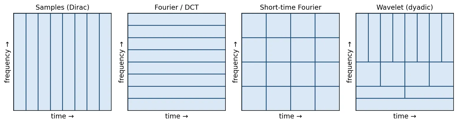
Figure 7.1 shows the four standard cases:

• Samples (the identity basis): perfect position, no frequency information.
• Fourier or DCT: perfect frequency, no position. A single sharp edge spreads over all coefficients.
• Short-time Fourier transform (STFT): cut the signal into windows and take a Fourier transform of each. Every tile has the same shape, chosen once for all frequencies [2].
• Wavelets: high-frequency tiles are narrow in time and tall in frequency; low-frequency tiles are wide and short. This matches natural images well: edges are brief, high-frequency events, while smooth shading is a slow, low-frequency one.

Basis images

Plain version: for a 2-D transform, each coefficient has its own little picture. The image is a weighted sum of those pictures, and the coefficient is the weight.

For a separable transform with matrix $\mathbf{A}$ whose $u$-th row is $\mathbf{a}_u^T$, rewrite the inverse as a sum of outer products:

$$\mathbf{F} = \sum_{u=0}^{N-1} \sum_{v=0}^{N-1} T(u, v)\, \mathbf{S}_{u,v}, \qquad \mathbf{S}_{u,v} = \mathbf{a}_u^{*} \mathbf{a}_v^{*T} .$$

Each $N \times N$ matrix $\mathbf{S}_{u,v}$ is a basis image. $T(u,v)$ tells you how much of basis image $(u, v)$ to add, $u$ indexes the vertical pattern and $v$ the horizontal one. Plotting all $N^2$ basis images side by side is the fastest way to understand what a transform “sees”.

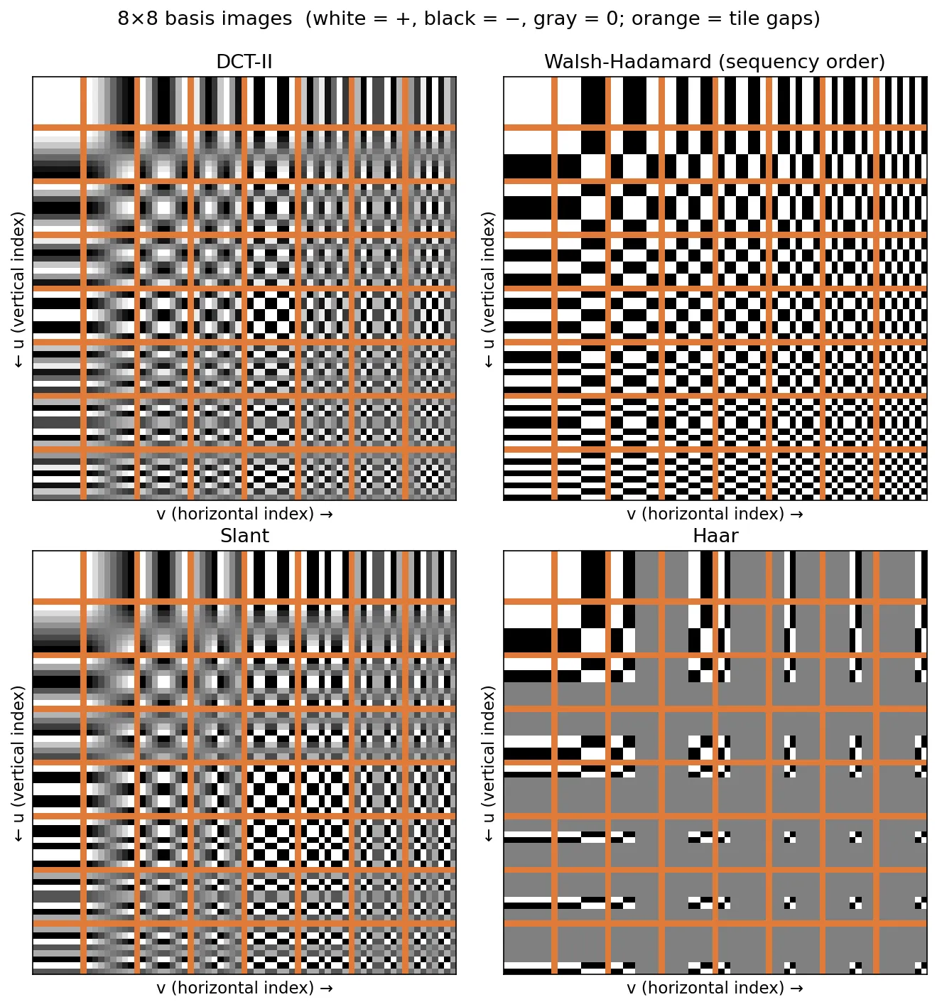
The top-left basis image is constant in all four transforms: it measures the average brightness, called the DC coefficient. Moving right or down, the patterns oscillate faster. The DCT oscillates smoothly, Walsh–Hadamard switches abruptly between $\pm 1$, slant adds linear ramps, and Haar confines each pattern to a small region of the tile.

Fourier-related transforms

Plain version: the Fourier family uses waves as building blocks. The cosine transform is the member that behaves best at the borders of a block, which is why your phone’s JPEG files use it.

The discrete Fourier transform, as a matrix

The 1-D DFT from Chapter 4 is a matrix transform with

$$A_{u,x} = \frac{1}{\sqrt{N}}\, e^{-j 2\pi u x / N}, \qquad u, x = 0, \dots, N-1 .$$

$A_{u,x}$ is the entry in row $u$, column $x$; $j = \sqrt{-1}$. With the $1/\sqrt{N}$ factor the matrix is unitary. Two drawbacks for compression: the coefficients are complex, and the DFT silently treats the signal as periodic. If the left and right borders of a block differ, the periodic extension has a jump, and a jump needs many high-frequency coefficients.

The discrete cosine transform

The (type-II) discrete cosine transform [3] uses real cosines:

$$t(u) = \alpha(u) \sum_{x=0}^{N-1} f(x) \cos\!\left[\frac{(2x+1)\,u\,\pi}{2N}\right], \qquad \alpha(0) = \sqrt{\tfrac{1}{N}},\;\; \alpha(u) = \sqrt{\tfrac{2}{N}} \text{ for } u \ge 1 .$$

Here $u$ is the frequency index and $\alpha(u)$ makes the basis orthonormal. The DCT equals (up to scaling) the DFT of a mirrored, even extension of the signal of length $2N$. Mirroring removes the border jump, so energy concentrates in fewer low-frequency coefficients. This energy compaction is the reason the JPEG standard applies an $8 \times 8$ DCT to image blocks [4]. Ahmed, Natarajan and Rao introduced the DCT in 1974 and showed that its performance compares closely with that of the Karhunen–Loève transform, the statistically optimal transform, in Wiener filtering and rate–distortion terms [3].

The discrete sine transform

The discrete sine transform uses sines instead. The type-I DST matrix is

$$A_{u,x} = \sqrt{\frac{2}{N+1}}\, \sin\!\left[\frac{(x+1)(u+1)\pi}{N+1}\right] ,$$

which corresponds to an odd extension of the signal. It is real, orthonormal and symmetric ($\mathbf{A} = \mathbf{A}^T = \mathbf{A}^{-1}$). It suits signals that are close to zero at both ends, such as prediction residuals. In SciPy it is scipy.fft.dst(x, type=1, norm="ortho").

Walsh–Hadamard transform

Plain version: build every basis vector from only $+1$ and $-1$. Then the transform needs no multiplications at all, just additions and subtractions.

The Hadamard matrix of order $N = 2^n$ is built recursively:

$$\mathbf{H}_1 = [\,1\,], \qquad \mathbf{H}_{2N} = \begin{bmatrix} \mathbf{H}_N & \mathbf{H}_N \\ \mathbf{H}_N & -\mathbf{H}_N \end{bmatrix}, \qquad \mathbf{A}_{\text{WHT}} = \frac{1}{\sqrt{N}}\,\mathbf{H}_N .$$

Every entry of $\mathbf{H}_N$ is $\pm 1$, and its rows are mutually orthogonal, so $\mathbf{A}_{\text{WHT}}$ is orthonormal (and symmetric). The rows of $\mathbf{H}_N$ come out in natural (Hadamard) order. For analysis it is nicer to reorder them by sequency, the number of sign changes along a row, which plays the role of frequency. Sequency-ordered rows are called Walsh functions, and Figure 7.2 shows their 2-D basis images.

The Walsh–Hadamard transform (WHT) was used for early image coding because it is cheap [5]. Its energy compaction is weaker than the DCT’s for natural images, because its square-wave basis approximates smooth shading poorly (see Figure 7.7 later). It remains useful where speed or hardware simplicity matters most, and as a building block for fast randomized algorithms.

import numpy as np
from scipy.linalg import hadamard

H = hadamard(8)                                    # natural (Hadamard) order
changes = (np.diff(np.sign(H), axis=1) != 0).sum(1)
W = H[np.argsort(changes)] / np.sqrt(8)            # sequency order
print((np.diff(np.sign(W), axis=1) != 0).sum(1))   # [0 1 2 3 4 5 6 7]

x = np.array([10, 12, 11, 13, 40, 42, 41, 43], float)
print(np.round(W @ x, 2))

The test signal is a step with small ripples. Its WHT is almost entirely in coefficient 0 (the mean) and coefficient 1 (a single sign change, matching the step); only a few small values remain.

Slant transform

Plain version: many image regions are not flat but get gradually brighter or darker. The slant transform includes a “ramp” building block so that such regions need only one or two coefficients.

Pratt, Chen and Welch designed the slant transform for image coding [6]. Like the WHT, it is orthonormal and built recursively, starting from $\mathbf{S}_2 = \frac{1}{\sqrt{2}}\begin{bmatrix}1 & 1 \\ 1 & -1\end{bmatrix}$:

$$\mathbf{S}_{N} = \frac{1}{\sqrt{2}}\, \mathbf{Q}_N \begin{bmatrix} \mathbf{S}_{N/2} & \mathbf{0} \\ \mathbf{0} & \mathbf{S}_{N/2} \end{bmatrix} ,$$

where $\mathbf{Q}_N$ is a sparse $N \times N$ mixing matrix. $\mathbf{Q}_N$ contains two constants,

$$a_N = \sqrt{\frac{3N^2}{4(N^2-1)}}, \qquad b_N = \sqrt{\frac{N^2-4}{4(N^2-1)}} ,$$

chosen so that the second row of $\mathbf{S}_N$ is a uniformly decreasing staircase (the “slant” vector) and the matrix stays orthonormal. The script for this chapter builds $\mathbf{S}_8$ this way and checks both properties numerically (scripts/figures/dip_ch07.py). In Figure 7.2 the slant basis images in the first row and first column are visible ramps. The transform has a fast algorithm of $O(N \log_2 N)$ operations, but in practice the DCT, which also handles ramps well, displaced it.

Haar transform

Plain version: take two neighbors, write down their average and their difference. Repeat on the averages. That is the Haar transform, and it is the simplest wavelet.

The Haar transform [1] uses basis functions that are either constant or a single up-down step, at different widths and positions. For $N = 2^n$ samples, index the functions by a scale $p$ and a position $q$, with $k = 2^p + q$ for $k \ge 1$. Up to normalization, the $k$-th basis vector equals $+1$ on the first half of the interval $\left[\frac{q}{2^p}, \frac{q+1}{2^p}\right)$, $-1$ on its second half, and 0 elsewhere (with positions measured as a fraction of the signal length). The $k = 0$ vector is constant. For $N = 4$,

$$\mathbf{A}_{\text{Haar}} = \begin{bmatrix} \tfrac{1}{2} & \tfrac{1}{2} & \tfrac{1}{2} & \tfrac{1}{2} \\[2pt] \tfrac{1}{2} & \tfrac{1}{2} & -\tfrac{1}{2} & -\tfrac{1}{2} \\[2pt] \tfrac{1}{\sqrt{2}} & -\tfrac{1}{\sqrt{2}} & 0 & 0 \\[2pt] 0 & 0 & \tfrac{1}{\sqrt{2}} & -\tfrac{1}{\sqrt{2}} \end{bmatrix} .$$

Rows 0 and 1 look at the whole signal; rows 2 and 3 each look at only one half. That is the key difference from every transform above: Haar basis functions are localized. A local event, such as an edge, changes only the few Haar coefficients whose support covers it. In the time–frequency picture, Haar has exactly the dyadic tiling of Figure 7.1. It is the bridge to the wavelet transforms that follow: the Haar transform is the discrete wavelet transform with the Haar wavelet.

Wavelet transforms

Plain version: look at the image at many zoom levels. At each level, keep a blurrier copy and write down only the details that the blurring removed. The blurry copies form a pyramid; the details are the wavelet coefficients.

Multiresolution analysis

Multiresolution analysis (MRA), formalized by Mallat [7], is the framework that turns this idea into a basis. Start with a scaling function $\varphi(x)$ and form shifted and scaled copies,

$$\varphi_{j,k}(x) = 2^{j/2}\, \varphi(2^j x - k) ,$$

where $j$ is the scale (larger $j$ means narrower functions and finer detail), $k$ is the integer shift, and $2^{j/2}$ keeps the energy at 1. Let $V_j$ be the space spanned by $\{\varphi_{j,k}\}_k$: all signals representable at resolution $j$. MRA requires four things:

1. The $\varphi_{0,k}$ are orthonormal (or at least a stable basis of $V_0$).
2. The spaces are nested, $\cdots \subset V_{-1} \subset V_0 \subset V_1 \subset \cdots$: anything visible at a coarse scale is also visible at a finer one.
3. The only function common to all $V_j$ is $f(x) = 0$.
4. Every square-integrable function can be approximated arbitrarily well as $j \to \infty$.

Because $V_0 \subset V_1$, the scaling function itself must be a combination of the finer ones. This gives the refinement equation (or dilation equation)

$$\varphi(x) = \sum_n h_\varphi(n)\, \sqrt{2}\, \varphi(2x - n) ,$$

where the coefficients $h_\varphi(n)$ are the scaling function coefficients. They will become a low-pass filter.

Wavelet functions

The details lost when going from $V_{j+1}$ down to $V_j$ live in a complementary space $W_j$, so that $V_{j+1} = V_j \oplus W_j$ (the symbol $\oplus$ means every element of $V_{j+1}$ splits uniquely into a part in $V_j$ and a part in $W_j$; for orthonormal wavelets the two parts are orthogonal). $W_j$ is spanned by the wavelet functions

$$\psi_{j,k}(x) = 2^{j/2}\, \psi(2^j x - k), \qquad \psi(x) = \sum_n h_\psi(n)\, \sqrt{2}\, \varphi(2x - n) .$$

For orthonormal wavelets, the wavelet function coefficients follow from the scaling coefficients by a modulation and time reversal, $h_\psi(n) = (-1)^n\, h_\varphi(1 - n)$. They form a high-pass filter. Repeating the split gives

$$L^2(\mathbb{R}) = V_{j_0} \oplus W_{j_0} \oplus W_{j_0+1} \oplus \cdots ,$$

where $L^2(\mathbb{R})$ is the space of finite-energy functions: one coarse approximation plus details at every finer scale.

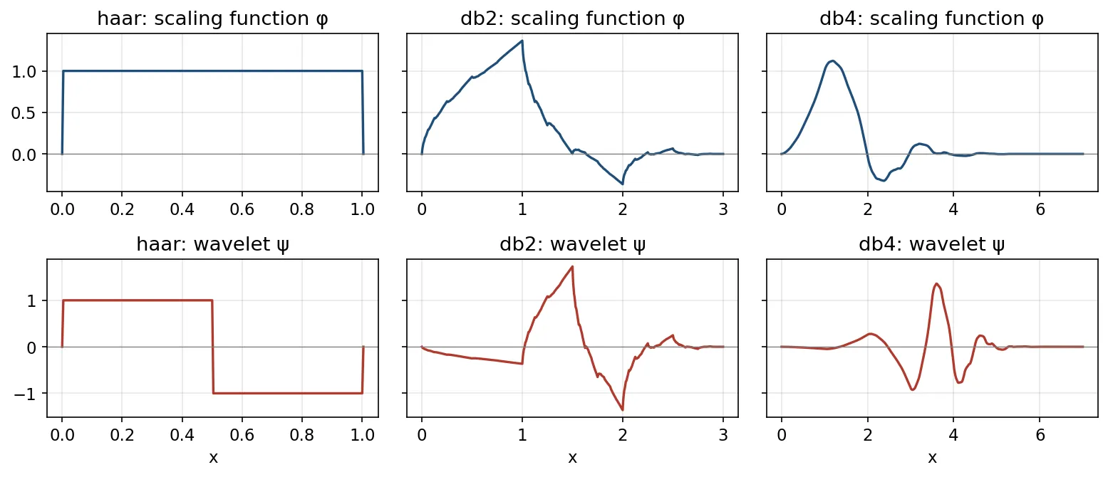
For Haar, $h_\varphi = [\tfrac{1}{\sqrt{2}}, \tfrac{1}{\sqrt{2}}]$ and $h_\psi = [\tfrac{1}{\sqrt{2}}, -\tfrac{1}{\sqrt{2}}]$: average and difference. Daubechies showed how to construct orthonormal wavelets with compact support (finite-length filters) and increasing smoothness; the regularity grows linearly with the filter length [8]. These are the dbN families in PyWavelets [10], where N is the number of vanishing moments: $\int x^m \psi(x)\,dx = 0$ for $m = 0, \dots, N-1$. A wavelet with $N$ vanishing moments ignores polynomials of degree below $N$, so smooth regions produce near-zero detail coefficients.

The wavelet series expansion

With these two families, a continuous signal $f(x)$ expands as

$$f(x) = \sum_k c_{j_0}(k)\, \varphi_{j_0,k}(x) + \sum_{j=j_0}^{\infty} \sum_k d_j(k)\, \psi_{j,k}(x) ,$$ $$c_{j_0}(k) = \langle f, \varphi_{j_0,k} \rangle, \qquad d_j(k) = \langle f, \psi_{j,k} \rangle .$$

$j_0$ is an arbitrary starting (coarsest) scale. The $c_{j_0}(k)$ are approximation (or scaling) coefficients and the $d_j(k)$ are detail (or wavelet) coefficients. Notice that every coefficient is again an inner product, exactly as in the Preliminaries. Unser and Blu explain where properties such as vanishing moments, approximation order and smoothness come from in this expansion [9].

The discrete wavelet transform in one dimension

For a sampled signal $f(x)$, $x = 0, \dots, M - 1$ with $M = 2^J$, the sums become finite:

$$W_\varphi(j_0, k) = \frac{1}{\sqrt{M}} \sum_{x} f(x)\, \varphi_{j_0,k}(x), \qquad W_\psi(j, k) = \frac{1}{\sqrt{M}} \sum_{x} f(x)\, \psi_{j,k}(x), \quad j \ge j_0 ,$$ $$f(x) = \frac{1}{\sqrt{M}} \left[ \sum_k W_\varphi(j_0, k)\, \varphi_{j_0,k}(x) + \sum_{j=j_0}^{J-1} \sum_k W_\psi(j, k)\, \psi_{j,k}(x) \right] .$$

$W_\varphi$ and $W_\psi$ are the approximation and detail coefficients of the discrete wavelet transform (DWT), and the $\varphi_{j,k}(x)$, $\psi_{j,k}(x)$ here are the continuous functions sampled at $x$. For an orthonormal wavelet the total number of coefficients equals $M$: the DWT is a change of basis, not an expansion.

The fast wavelet transform

Plain version: you never need to evaluate $\varphi$ or $\psi$. Two short filters and “keep every second sample” do all the work, level after level.

Substituting the refinement equations into the DWT gives Mallat’s pyramid algorithm, now called the fast wavelet transform (FWT) [7]:

$$W_\psi(j, k) = \sum_n h_\psi(n - 2k)\, W_\varphi(j+1, n), \qquad W_\varphi(j, k) = \sum_n h_\varphi(n - 2k)\, W_\varphi(j+1, n) .$$

Read it as: correlate the finer approximation $W_\varphi(j+1, \cdot)$ with $h_\psi$ (or $h_\varphi$), then keep every second output (downsampling by 2). In signal-processing terms this is a two-channel analysis filter bank: a low-pass branch produces the next approximation and a high-pass branch produces the details. Feed the low-pass output into the same bank again, and so on. Each level halves the data, so the total cost is $O(M)$, faster than the FFT’s $O(M \log M)$.

The inverse FWT is a synthesis filter bank: upsample each branch by 2 (insert zeros), filter with the synthesis filters, and add. For orthonormal wavelets the synthesis filters are the time-reversed analysis filters, and the bank achieves perfect reconstruction: the output equals the input exactly, despite the aliasing introduced by downsampling in each branch, because the aliasing terms of the two branches cancel. Vetterli and Kovačević’s textbook develops this subband-coding view in depth [2].

import numpy as np
import pywt

x = np.array([4.0, 6.0, 10.0, 12.0, 8.0, 6.0, 5.0, 5.0])
w = pywt.Wavelet("haar")
h0, h1 = np.array(w.dec_lo), np.array(w.dec_hi)   # [.707 .707], [-.707 .707]

def analysis(x):
    lo = np.convolve(x, h0)[1::2]   # filter, then keep every 2nd sample
    hi = np.convolve(x, h1)[1::2]
    return lo, hi

a1, d1 = analysis(x)
a2, d2 = analysis(a1)
print("a2", a2, "d2", d2, "d1", d1.round(3))

ref = pywt.wavedec(x, "haar", level=2)            # [a2, d2, d1]
print(all(np.allclose(p, q) for p, q in zip(ref, [a2, d2, d1])))
print(np.allclose(pywt.waverec(ref, "haar"), x))

The two-line filter bank reproduces pywt.wavedec exactly. Note how the detail coefficient is 0 for the pair (5, 5): no change, no detail.

Wavelet transforms in two dimensions

Plain version: run the 1-D filter bank along the rows, then along the columns. You get one small blurry image and three “edge maps”, one per direction.

The 2-D DWT is separable. One level uses a 2-D scaling function and three 2-D wavelets, each a product of 1-D functions:

$$\varphi(x, y) = \varphi(x)\varphi(y), \quad \psi^H(x, y) = \psi(x)\varphi(y), \quad \psi^V(x, y) = \varphi(x)\psi(y), \quad \psi^D(x, y) = \psi(x)\psi(y) .$$

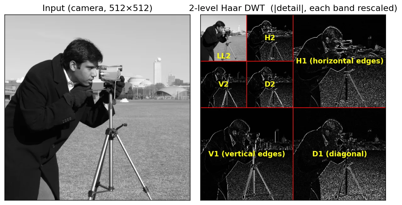
Here $x$ is the row index (vertical position) and $y$ the column index, following the book’s convention. $\psi^H$ changes along the vertical direction and is smooth horizontally, so it responds to horizontal edges. $\psi^V$ responds to vertical edges, and $\psi^D$ to diagonal detail and corners. One level turns an $M \times N$ image into four $\frac{M}{2} \times \frac{N}{2}$ subbands:

Subband	Rows filter	Columns filter	Often called	PyWavelets name
Approximation	low	low	LL	cA
Horizontal detail	high	low	LH or HL (conventions differ)	cH
Vertical detail	low	high	HL or LH	cV
Diagonal detail	high	high	HH	cD

“Rows filter” here means the filter applied across rows, that is, along the vertical direction. Because the LH/HL labels are swapped between textbooks and libraries, this chapter uses the unambiguous names H, V and D. Repeating the decomposition on the approximation band gives the familiar nested layout in Figure 7.4.

import numpy as np
import pywt
from skimage import data, img_as_float

img = img_as_float(data.camera())
LL1, (H1, V1, D1) = pywt.dwt2(img, "haar")   # one level
LL2, (H2, V2, D2) = pywt.dwt2(LL1, "haar")   # second level on LL1
print(img.shape, LL1.shape, LL2.shape)       # (512, 512) (256, 256) (128, 128)

e = lambda a: float((a ** 2).sum())
total = e(img)
print(f"energy in LL2: {e(LL2) / total:.4f}")

coeffs = pywt.wavedec2(img, "haar", level=2)  # same thing in one call
print(np.allclose(pywt.waverec2(coeffs, "haar"), img))

After two levels, the $128 \times 128$ approximation, one sixteenth of the coefficients, holds about 99% of the energy of the camera image. The other 15/16 of the coefficients are mostly near zero, which is exactly the sparsity that compression and denoising exploit.

Wavelet packets

The standard DWT only splits the low-pass band again. A wavelet packet decomposition splits every band, detail bands included, producing a full binary tree (a quadtree in 2-D). After $L$ levels a 2-D packet tree has $4^L$ leaves. Any choice of nodes that covers the frequency axis without overlap is a valid orthonormal basis, so the tree is a library of bases. Coifman and Wickerhauser’s best-basis algorithm searches this library efficiently, choosing the basis that minimizes an additive cost such as the entropy of the normalized coefficients [11]. Packets help for textures, which carry a lot of energy at mid and high frequencies that the plain DWT leaves in a single wide band.

import pywt
from skimage import data, img_as_float

img = img_as_float(data.camera())
wp = pywt.WaveletPacket2D(img, "haar", maxlevel=2)
print([n.path for n in wp.get_level(2)][:6], len(wp.get_level(2)))  # 16 subbands

Node paths spell out the branch taken at each level (a approximation, h, v, d details), so "hd" is the diagonal detail of the horizontal-detail band.

Applications

Denoising by thresholding

Plain version: in the wavelet domain, a clean image is a few large numbers, while white noise is many small numbers spread everywhere. Set the small ones to zero and transform back.

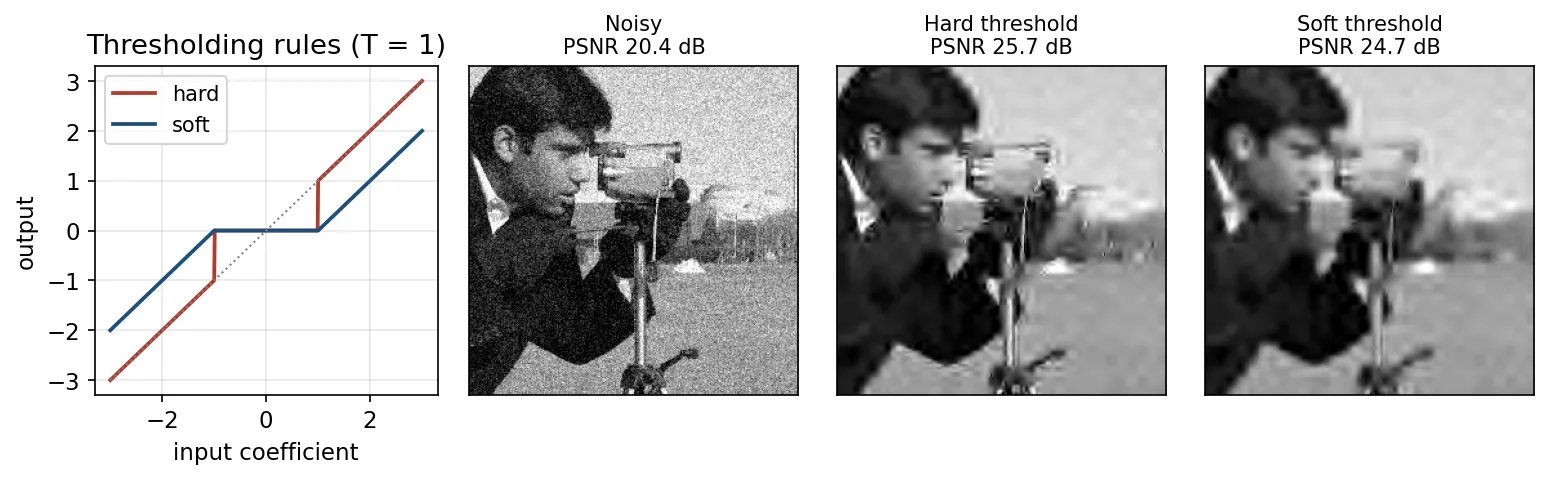
An orthonormal transform maps white Gaussian noise of standard deviation $\sigma$ to white Gaussian noise of the same $\sigma$ in every subband, while the image’s energy concentrates in few coefficients. Thresholding rules for a detail coefficient $w$ and threshold $T$:

$$\eta_{\text{hard}}(w) = \begin{cases} w, & |w| > T \\ 0, & |w| \le T \end{cases} \qquad \eta_{\text{soft}}(w) = \operatorname{sign}(w)\, \max(|w| - T,\, 0) .$$

Hard thresholding keeps or kills. Soft thresholding also shrinks the survivors toward zero by $T$, which gives a continuous rule with fewer artifacts but some loss of contrast. Two classic choices of $T$:

• Universal threshold (VisuShrink), $T = \sigma\sqrt{2 \ln n}$ for $n$ samples, from Donoho and Johnstone [12]. Donoho showed that soft thresholding with this $T$ gives, with high probability, an estimate that is at least as smooth as the true signal [13]. The noise level is usually estimated robustly from the finest diagonal band as $\hat{\sigma} = \operatorname{median}(|w|)/0.6745$ [12].
• BayesShrink, from Chang, Yu and Vetterli, sets a separate threshold for each subband, $T = \hat{\sigma}^2 / \hat{\sigma}_X$, where $\hat{\sigma}_X$ is the estimated standard deviation of the clean coefficients in that band [14]. It adapts to how much signal each band contains and usually beats the universal threshold.

import numpy as np
import pywt
from skimage import data, img_as_float
from skimage.metrics import peak_signal_noise_ratio as psnr

rng = np.random.default_rng(7)
clean = img_as_float(data.camera())
noisy = clean + rng.normal(0, 0.1, clean.shape)

def wavelet_denoise(y, wavelet="db4", level=3, mode="soft"):
    c = pywt.wavedec2(y, wavelet, mode="periodization", level=level)
    sigma = np.median(np.abs(c[-1][2])) / 0.6745       # noise level from finest HH
    T = sigma * np.sqrt(2 * np.log(y.size))            # universal threshold
    c = [c[0]] + [tuple(pywt.threshold(d, T, mode) for d in lvl) for lvl in c[1:]]
    return pywt.waverec2(c, wavelet, mode="periodization")

for mode in ["hard", "soft"]:
    out = np.clip(wavelet_denoise(noisy, mode=mode), 0, 1)
    print(mode, round(psnr(clean, out, data_range=1), 1), "dB")
print("noisy", round(psnr(clean, np.clip(noisy, 0, 1), data_range=1), 1), "dB")

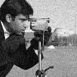
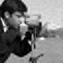
On this example the noisy image scores 20.4 dB PSNR, hard thresholding 25.7 dB and soft thresholding 24.7 dB. The universal threshold is conservative (it is designed to remove essentially all the noise), so with soft shrinkage on top it over-smooths; the cartoon-like look in Figure 7.5 is the price. Subband-adaptive thresholds such as BayesShrink, or an undecimated (shift-invariant) transform, reduce both the blur and the blocky artifacts. scikit-image wraps these variants in skimage.restoration.denoise_wavelet.

Drag the slider to compare the noisy input with the soft-thresholded result:

NoisySoft threshold

Edge detection

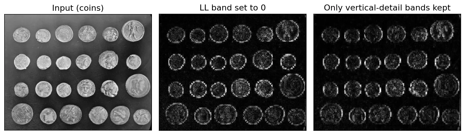
Because the detail bands are high-pass responses in three directions, wavelets give a quick edge detector: set the approximation band to zero and invert the transform. What remains is the image minus its coarse version, which is concentrated at edges. Keeping only some detail bands selects edge orientation, as in Figure 7.6. Coarser levels give thicker but more noise-robust edges, a multiscale behavior similar to choosing the $\sigma$ of a Gaussian-derivative edge detector.

Compression preview

Compression rests on energy compaction: transform, keep the few big coefficients, and code them efficiently. Figure 7.7 keeps only the largest 5% of coefficients of the whole $512 \times 512$ image for four transforms. The two wavelets win by more than 2 dB over the DCT and more than 4 dB over the WHT, and their errors look different: the Fourier-type bases ring around edges and lose texture everywhere, while wavelets keep edges crisp and lose detail mainly in smooth or textured regions.

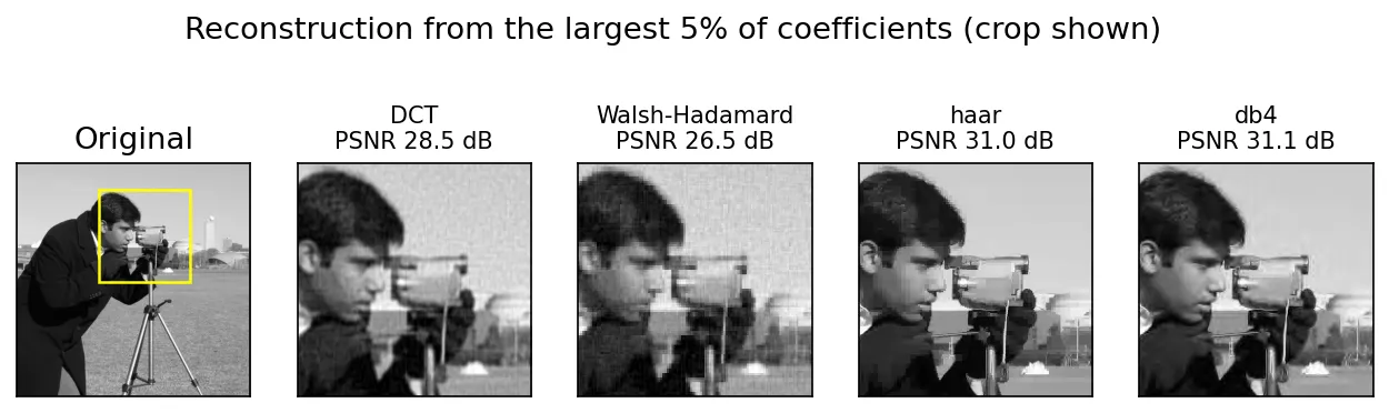
Real codecs are more careful than “keep the top 5%”. JPEG uses a block DCT with quantization and entropy coding [4], and JPEG 2000 uses a multilevel 2-D DWT with biorthogonal filters, followed by bit-plane coding of each subband [15]. Chapter 8 covers these pipelines in detail.

Modern view

Wavelets arrived in image processing in the late 1980s as a unifying theory, peaked in the 1990s and 2000s as the backbone of denoising and JPEG 2000, and are now mostly an ingredient: of sparse models, of signal-processing-inspired network layers, and of efficient generative models. Here are the surveys and landmark papers worth reading, and what each contributes.

Foundations: Mallat (1989) and Daubechies (1988). Mallat’s paper [7] introduced multiresolution analysis for images, the link between orthonormal wavelets and two-channel filter banks, and the pyramid algorithm that makes the transform $O(N)$. It also introduced the 2-D separable decomposition into horizontal, vertical and diagonal bands that every library still uses. Daubechies [8] provided the missing piece: orthonormal wavelets with compact support and a chosen amount of smoothness, which made the filters short and practical. Together they explain why pywt.wavedec2(img, "db4") exists at all.

Textbook-length survey: Vetterli and Kovačević (1995). Wavelets and Subband Coding [2] builds the theory from the signal-processing side: filter banks, perfect reconstruction, time–frequency tilings, and coding. The authors bought back the copyright and distribute the book freely, which makes it the best open reference for the filter-bank view in this chapter.

What makes a wavelet good: Unser and Blu (2003). “Wavelet theory demystified” [9] rebuilds the classical theory in a self-contained way by writing any scaling function as a B-spline convolved with a residual “irregular” part. Its main takeaway is that the B-spline factor alone is responsible for five properties practitioners care about: order of approximation, reproduction of polynomials, vanishing moments, the multiscale differentiation property, and smoothness. If you want to know why db4 behaves better than Haar on smooth images, this is the paper that explains it.

From bases to dictionaries: Rubinstein, Bruckstein and Elad (2010). “Dictionaries for sparse representation modeling” [16] surveys the move from analytic transforms (Fourier, DCT, wavelets and their directional successors) to dictionaries learned from data. Its takeaway is the bridge to modern methods: the wavelet idea of “a few coefficients explain the image” survived, but the basis became something you can train. This line of work leads directly into learned priors for restoration.

The standard in practice: Skodras, Christopoulos and Ebrahimi (2001). Their overview of JPEG 2000 [15] shows how the DWT, biorthogonal filters, subband quantization and embedded coding fit together in a real codec, and what features (resolution scalability, region-of-interest coding, lossless mode) multiresolution makes possible.

Classical denoising theory: Donoho and Johnstone; Chang, Yu and Vetterli. The shrinkage papers [12], [13], [14] showed that a simple nonlinearity in the wavelet domain is close to optimal over broad classes of signals, and that adapting the threshold per subband helps in practice. Every “denoise by thresholding a transform” method, including many hand-crafted priors used before deep learning, descends from these results.

What deep learning changed, and what it did not

Scattering networks. Bruna and Mallat’s wavelet scattering transform [17] cascades wavelet convolutions with a modulus nonlinearity and averaging. It is a convolutional network whose filters are fixed wavelets rather than learned, and the authors prove that it is stable to small deformations and locally translation invariant. The first layer behaves like SIFT-type descriptors, and higher layers add information that can tell apart textures with the same Fourier power spectrum. It gave state-of-the-art results on handwritten digit and texture classification at the time and became a reference point for explaining why CNNs work: a wavelet frame (redundant, as in the Preliminaries) plus a simple nonlinearity already yields invariance.

Wavelets as pooling and downsampling layers. Strided convolution and max-pooling downsample without proper low-pass filtering, so they alias. Li et al. replaced these operations with DWT layers in standard classifiers (WaveCNet) and kept only the low-frequency band, which improved robustness to noise [19]. In restoration, Liu et al.’s MWCNN replaces the pooling and unpooling of a U-Net with the 2-D DWT and its inverse [18]. Because the DWT is invertible, no information is lost when the network shrinks the feature maps, and the network gets a large receptive field cheaply. The same idea, an invertible and alias-aware down-sampler, appears in many later restoration and generation models.

Large receptive fields. Finder et al.’s WTConv layer (ECCV 2024) applies small convolutions to the subbands of a multilevel DWT, so the effective receptive field grows exponentially with the number of levels while parameters grow only logarithmically with kernel size [20]. It works as a drop-in layer in architectures such as ConvNeXt and MobileNetV2, and the authors report better robustness to image corruptions and a stronger response to shapes over textures.

What did not change. The DCT still sits inside JPEG, and the DCT and its integer approximations remain core tools in conventional image and video codecs. Hand-tuned wavelet thresholding has been overtaken in denoising quality by trained networks, but it is still the fastest strong baseline, needs no training data, and has guarantees. Most importantly, the vocabulary of this chapter (bases, frames, filter banks, multiresolution, aliasing, sparsity) is the vocabulary used to analyze what convolutional networks do.

Key takeaways

• A linear transform is a change of basis. Each coefficient is an inner product, that is, a correlation of the image with one basis function.
• Orthonormal transforms are matrix products, $\mathbf{T} = \mathbf{A}\mathbf{F}\mathbf{A}^T$ for separable 2-D cases, with the transpose as the inverse and energy preserved.
• The DCT compacts the energy of smooth images better than the DFT or WHT because its implied even extension has no border jump; this is why JPEG uses it.
• WHT and slant transforms trade some compaction for simplicity (only $\pm 1$) or for an explicit ramp vector; Haar adds localization.
• The time–frequency plane shows the trade-off: Fourier bases are sharp in frequency, samples sharp in time, wavelets adapt the tile shape to the frequency.
• Multiresolution analysis turns two short filters into a fast $O(N)$ wavelet transform. In 2-D it yields an approximation band and horizontal, vertical and diagonal detail bands at each level.
• Sparsity in the wavelet domain powers denoising (hard/soft thresholding), quick edge maps and compression (JPEG 2000).
• Modern networks reuse wavelets as fixed feature extractors (scattering), as invertible down-samplers (MWCNN, WaveCNet) and as cheap large-receptive-field layers (WTConv).

Exercises

1. A frame by hand. Take the three unit vectors in the plane at angles 90°, 210° and 330°. Compute $\sum_k \langle \mathbf{f}, \mathbf{s}_k \rangle^2$ for $\mathbf{f} = (1, 0)$ and for $\mathbf{f} = (0, 1)$. What are the frame bounds, and how do you reconstruct $\mathbf{f}$ from its three coefficients?

Hint

Both sums equal $3/2$; in fact, for every unit $\mathbf{f}$ the sum is $3/2$, so the frame is tight with $A = B = 3/2$. Reconstruct with $\mathbf{f} = \frac{2}{3}\sum_k \langle \mathbf{f}, \mathbf{s}_k \rangle \mathbf{s}_k$.

2. Separable cost. For a $256 \times 256$ image, count the multiplications for (a) a general 2-D linear transform written as one $65536 \times 65536$ matrix, (b) the separable form $\mathbf{A}\mathbf{F}\mathbf{A}^T$ with dense $\mathbf{A}$, and (c) a three-level Haar FWT.

Hint

(a) $N^4 \approx 4.3 \times 10^9$. (b) two products of $N^3$ each, $2N^3 \approx 3.4 \times 10^7$. (c) Each level filters every row and column of the current approximation with 2-tap filters at half rate; the total is a small constant times $N^2$, a few hundred thousand.

3. Why mirror? Take $f = [1, 2, 3, 4, 5, 6, 7, 8]$ (a ramp). Compute its DFT and its DCT with SciPy and count how many coefficients you need to capture 99% of the energy in each. Explain the difference using the implied periodic and even extensions.

Hint

The periodic extension jumps from 8 back to 1, which needs many DFT harmonics. The even extension $\ldots 2, 1, 1, 2, \ldots, 8, 8, 7, \ldots$ is continuous, so the DCT needs only two or three coefficients.

4. Haar by hand. Compute a two-level Haar DWT of $[2, 2, 6, 6, 3, 5, 9, 9]$ using averages and differences scaled by $1/\sqrt{2}$. Which detail coefficients are zero, and why? Check your answer with pywt.wavedec.

Hint

Level 1 pairs: (2,2), (6,6), (3,5), (9,9). Only the pair (3,5) has a non-zero difference. At level 2, compare the scaled sums of neighboring pairs. Watch PyWavelets’ sign convention: with its Haar filters, each detail coefficient comes out as (first − second)$/\sqrt{2}$, so the pair (3, 5) gives $-\sqrt{2}$.

5. Thresholds in practice. Modify the denoising code to use (a) a threshold equal to $3\hat{\sigma}$, and (b) a per-subband BayesShrink threshold $\hat{\sigma}^2 / \hat{\sigma}_X$ with $\hat{\sigma}_X = \sqrt{\max(\overline{w^2} - \hat{\sigma}^2, 0)}$ computed in each band. Compare PSNR with the universal threshold for $\sigma = 0.05$ and $\sigma = 0.2$.

Hint

The universal threshold for a $512 \times 512$ image is about $5\hat{\sigma}$, so (a) keeps more coefficients. Expect (b) to be the best of the three for soft thresholding. If $\hat{\sigma}_X = 0$, set the band to zero.

6. Shift sensitivity. Shift the camera image by one pixel horizontally, take a one-level Haar DWT of both versions, and compare the energy in the V band. Why does a one-pixel shift change the coefficients so much, and how would an undecimated transform (pywt.swt2) behave?

Hint

Downsampling by 2 makes the DWT shift-variant: an edge that falls inside a Haar pair produces a detail coefficient, while the same edge falling between pairs produces none. The stationary (undecimated) transform skips downsampling, so it is a redundant frame and shifts its coefficients along with the image.

References

1. R. C. Gonzalez and R. E. Woods, Digital Image Processing, 4th ed., Pearson, 2018, Ch. 7. publisher page
2. M. Vetterli and J. Kovačević, Wavelets and Subband Coding, Prentice Hall, 1995 (free edition from the authors). book site
3. N. Ahmed, T. Natarajan and K. R. Rao, “Discrete Cosine Transform,” IEEE Transactions on Computers, 1974. doi
4. G. K. Wallace, “The JPEG still picture compression standard,” IEEE Transactions on Consumer Electronics, 1992. doi
5. W. K. Pratt, J. Kane and H. C. Andrews, “Hadamard transform image coding,” Proceedings of the IEEE, 1969. doi
6. W. K. Pratt, W.-H. Chen and L. R. Welch, “Slant transform image coding,” IEEE Transactions on Communications, 1974. doi
7. S. G. Mallat, “A theory for multiresolution signal decomposition: the wavelet representation,” IEEE Transactions on Pattern Analysis and Machine Intelligence, 1989. doi
8. I. Daubechies, “Orthonormal bases of compactly supported wavelets,” Communications on Pure and Applied Mathematics, 1988. doi
9. M. Unser and T. Blu, “Wavelet theory demystified,” IEEE Transactions on Signal Processing, 2003. doi
10. G. R. Lee, R. Gommers, F. Waselewski, K. Wohlfahrt and A. O’Leary, “PyWavelets: A Python package for wavelet analysis,” Journal of Open Source Software, 2019. doi
11. R. R. Coifman and M. V. Wickerhauser, “Entropy-based algorithms for best basis selection,” IEEE Transactions on Information Theory, 1992. doi
12. D. L. Donoho and I. M. Johnstone, “Ideal spatial adaptation by wavelet shrinkage,” Biometrika, 1994. doi
13. D. L. Donoho, “De-noising by soft-thresholding,” IEEE Transactions on Information Theory, 1995. doi
14. S. G. Chang, B. Yu and M. Vetterli, “Adaptive wavelet thresholding for image denoising and compression,” IEEE Transactions on Image Processing, 2000. doi
15. A. Skodras, C. Christopoulos and T. Ebrahimi, “The JPEG 2000 still image compression standard,” IEEE Signal Processing Magazine, 2001. doi
16. R. Rubinstein, A. M. Bruckstein and M. Elad, “Dictionaries for sparse representation modeling,” Proceedings of the IEEE, 2010. doi
17. J. Bruna and S. Mallat, “Invariant scattering convolution networks,” arXiv:1203.1513, 2012. arXiv
18. P. Liu, H. Zhang, K. Zhang, L. Lin and W. Zuo, “Multi-level wavelet-CNN for image restoration,” CVPR Workshops (NTIRE), 2018. arXiv
19. Q. Li, L. Shen, S. Guo and Z. Lai, “Wavelet integrated CNNs for noise-robust image classification,” CVPR, 2020. arXiv
20. S. E. Finder, R. Amoyal, E. Treister and O. Freifeld, “Wavelet convolutions for large receptive fields,” ECCV, 2024. arXiv