Chapter 5 · Image Restoration and Reconstruction

What you’ll learn

• How to write image damage as a model, $g = h \star f + \eta$, and why that model separates restoration from enhancement
• The common noise models, how to recognise them from a histogram, and how to measure their parameters from a flat patch
• Which spatial filter to use for which noise: mean filters, order-statistic filters, and adaptive filters
• How to remove periodic interference with notch filters in the frequency domain
• How to estimate a blur and undo it with inverse, Wiener, constrained least squares and geometric mean filters, and why the naive inverse fails
• How a CT scanner turns a set of 1-D projections into a 2-D slice: the Radon transform, the Fourier-slice theorem and filtered backprojection

The big picture

Chapter 3 and Chapter 4 improved images so they look better. This chapter asks a stricter question: what did the image look like before it was damaged? To answer it we need a model of the damage. Once we have the model, undoing it becomes a well-posed (or at least a well-understood) mathematical problem. The chapter follows the arrangement of Gonzalez and Woods [1].

Restoration matters wherever the true scene is what counts: astronomy, microscopy, forensic photos, medical imaging and every phone camera pipeline. The last part of the chapter, reconstruction from projections, is the same idea pushed to the extreme. A CT scanner never sees the slice at all. It sees only shadows of it from many angles, and we must reconstruct the slice from them.

A model of the image degradation/restoration process

In plain words: the camera sees a slightly blurred copy of the scene, and then random noise is added on top. Restoration tries to get back the scene.

We write the degradation as

$$g(x, y) = h(x, y) \star f(x, y) + \eta(x, y),$$

where $f(x,y)$ is the ideal (unknown) image, $h(x,y)$ is the degradation function, also called the point spread function (PSF), $\star$ is 2-D convolution, $\eta(x,y)$ is additive noise, and $g(x,y)$ is the image we actually observe. By the convolution theorem from Chapter 4, the same model in the frequency domain is

$$G(u, v) = H(u, v)\, F(u, v) + N(u, v),$$

where capital letters denote the 2-D discrete Fourier transforms (DFTs) of the matching lower-case functions, and $(u, v)$ are frequency coordinates. $H(u,v)$ is called the optical transfer function (OTF).

The goal of restoration is an estimate $\hat f(x,y)$ that is as close as possible to $f(x,y)$. The more we know about $h$ and $\eta$, the closer we can get.

Restoration versus enhancement

Enhancement (Chapter 3 and 4) is largely subjective: we change contrast or sharpen until the result looks good to a viewer. Restoration is objective: it uses a model of the degradation and judges the result by how close it gets to the true image, usually with a measurable criterion such as mean squared error. Some tools appear in both chapters (a median filter, for instance), but the reason for using them differs. In restoration we pick the filter because the noise model tells us it is the right one.

This chapter first handles the case $h = \delta$ (no blur, only noise), then adds blur.

Noise models

In plain words: noise is the random “grain” on top of the picture. Different sensors and situations produce different kinds of grain, and each kind has its own fingerprint in the histogram.

Spatial and frequency properties of noise

Two questions describe noise. Spatially, is the noise at one pixel related to the noise at its neighbours, and is it related to the image itself? In this chapter we assume, unless stated otherwise, that noise is independent of position and uncorrelated with the image. In frequency, how is the noise power spread across $(u,v)$? Noise whose Fourier spectrum is roughly constant is called white noise, by analogy with white light containing all visible frequencies. Periodic noise is the opposite: its power sits at a few isolated frequencies.

Under these assumptions the noise is fully described by the probability density function (PDF) of its values, written $p(z)$, where $z$ is an intensity.

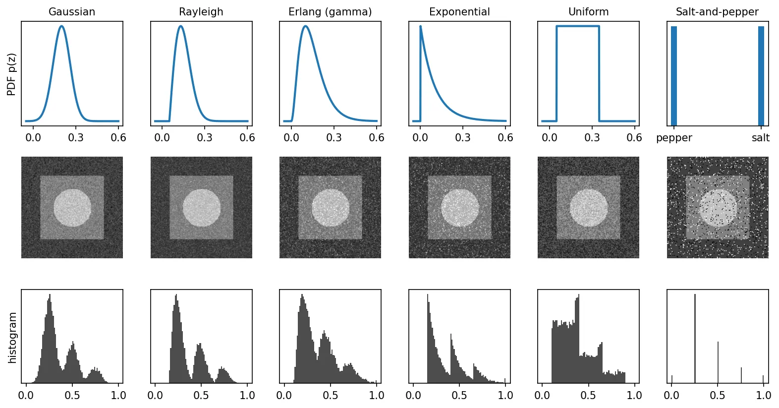
The common PDFs

Gaussian. The most widely used model, because it is mathematically convenient and fits electronic sensor noise well:

$$p(z) = \frac{1}{\sqrt{2\pi}\,\sigma}\, e^{-(z - \bar z)^2 / 2\sigma^2},$$

where $\bar z$ is the mean and $\sigma$ the standard deviation (so $\sigma^2$ is the variance). About 68% of values fall within $\bar z \pm \sigma$ and about 95% within $\bar z \pm 2\sigma$.

Rayleigh. A one-sided, skewed density that describes noise in range imaging:

$$p(z) = \begin{cases} \dfrac{2}{b}(z - a)\, e^{-(z-a)^2/b}, & z \ge a \\[4pt] 0, & z < a \end{cases} \qquad \bar z = a + \sqrt{\pi b / 4}, \quad \sigma^2 = \frac{b(4 - \pi)}{4},$$

where $a$ shifts the starting point and $b > 0$ controls the spread.

Erlang (gamma). Also skewed, with a longer tail:

$$p(z) = \begin{cases} \dfrac{a^b z^{b-1}}{(b-1)!}\, e^{-a z}, & z \ge 0 \\[4pt] 0, & z < 0 \end{cases} \qquad \bar z = \frac{b}{a}, \quad \sigma^2 = \frac{b}{a^2},$$

where $a > 0$ is a rate and $b$ is a positive integer (the shape). Allowing non-integer $b$ gives the general gamma density.

Exponential. The Erlang density with $b = 1$:

$$p(z) = a\, e^{-a z} \ (z \ge 0), \qquad \bar z = \frac{1}{a}, \quad \sigma^2 = \frac{1}{a^2}.$$

It appears in laser imaging (speckle intensity).

Uniform. Every value in an interval $[a, b]$ is equally likely:

$$p(z) = \frac{1}{b - a} \ (a \le z \le b), \qquad \bar z = \frac{a + b}{2}, \quad \sigma^2 = \frac{(b - a)^2}{12}.$$

It is mainly useful for simulations (quantization error is approximately uniform).

Salt-and-pepper (impulse) noise. A pixel is either untouched, or replaced by a very bright value (salt) with probability $P_s$, or by a very dark value (pepper) with probability $P_p$. The total fraction of corrupted pixels is $P = P_s + P_p$, called the noise density. Faulty sensor elements and transmission bit errors produce this kind of noise. Unlike the others, it is not additive: it replaces pixel values.

Periodic noise

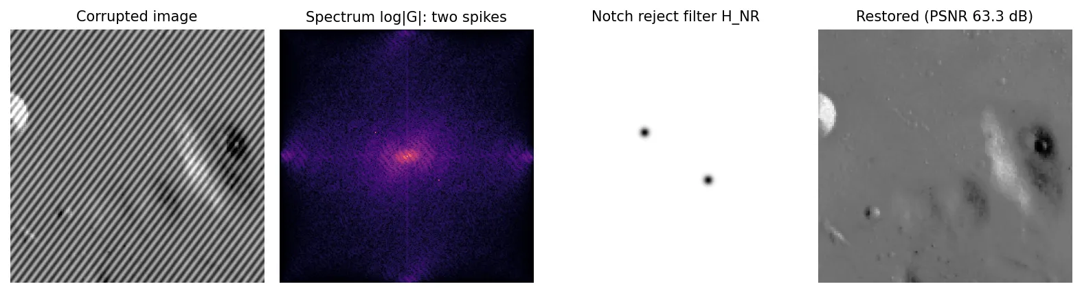
Electrical or electromechanical interference during image capture can add a sinusoid such as $A \sin(2\pi(u_0 x / M + v_0 y / N))$ to the image, where $A$ is its amplitude, $(u_0, v_0)$ its frequency, and $M \times N$ the image size. It is spatially dependent, so a PDF does not describe it. In the Fourier spectrum, however, each sinusoid is a pair of bright spikes at $\pm(u_0, v_0)$, which makes it easy to remove there (see the section on periodic noise reduction below).

Estimating noise parameters

If you can control the imaging system, photograph a flat, uniformly lit target: everything you see is noise. If you only have the images, find a small region $S$ that should be constant (sky, a blank wall, the background) and compute its histogram $p_S(z_i)$, the fraction of pixels in $S$ with intensity $z_i$. Then

$$\bar z = \sum_{i} z_i\, p_S(z_i), \qquad \sigma^2 = \sum_{i} (z_i - \bar z)^2\, p_S(z_i).$$

The shape of the patch histogram tells you which PDF to use. The mean and variance then give the parameters ($a$ and $b$ for Rayleigh, Erlang, and so on). For impulse noise, count the pixels at the extreme values to estimate $P_s$ and $P_p$.

import numpy as np
from skimage import data, img_as_float

rng = np.random.default_rng(0)
f = img_as_float(data.camera())                  # values in [0, 1]

g_gauss = f + rng.normal(0.0, 0.05, f.shape)     # additive Gaussian, sigma = 0.05
g_unif = f + rng.uniform(-0.1, 0.1, f.shape)     # additive uniform on [-0.1, 0.1]
g_sp = f.copy()
r = rng.random(f.shape)
g_sp[r < 0.05] = 0.0                             # 5 % pepper
g_sp[r > 0.95] = 1.0                             # 5 % salt

# Estimate the noise from a patch that should be flat (here: sky, top-left)
patch = g_gauss[10:60, 10:60]
print(f"mean = {patch.mean():.3f}, std = {patch.std():.3f}")   # std close to 0.05

Restoration in the presence of noise only — spatial filtering

In plain words: when the only problem is noise, replace every pixel by a smart summary of its neighbourhood. The best summary depends on the kind of noise.

With no blur, the model reduces to $g(x,y) = f(x,y) + \eta(x,y)$ (or, for impulse noise, a replacement). Below, $S_{xy}$ is an $m \times n$ window centred at $(x,y)$, and $(r, c)$ runs over the pixels in it.

Mean filters

Arithmetic mean — the plain average:

$$\hat f(x, y) = \frac{1}{mn} \sum_{(r,c) \in S_{xy}} g(r, c).$$

It reduces Gaussian or uniform noise but blurs edges.

Geometric mean — the $mn$-th root of the product:

$$\hat f(x, y) = \Bigl[\prod_{(r,c) \in S_{xy}} g(r, c)\Bigr]^{1/mn}.$$

Smoothing is similar to the arithmetic mean, but less detail is lost.

Harmonic mean:

$$\hat f(x, y) = \frac{mn}{\sum_{(r,c) \in S_{xy}} 1 / g(r, c)}.$$

It handles salt noise and Gaussian-like noise well but fails badly on pepper noise, because a single near-zero pixel dominates the sum of reciprocals.

Contraharmonic mean of order $Q$:

$$\hat f(x, y) = \frac{\sum_{(r,c) \in S_{xy}} g(r, c)^{Q+1}}{\sum_{(r,c) \in S_{xy}} g(r, c)^{Q}}.$$

Here $Q$ is the order. Positive $Q$ removes pepper noise, negative $Q$ removes salt noise, and it cannot remove both at once. $Q = 0$ gives the arithmetic mean and $Q = -1$ the harmonic mean. Using the wrong sign is disastrous, as Figure 5.2 shows.

Order-statistic filters

These filters sort the pixels in $S_{xy}$ and pick from the sorted list.

• Median: $\hat f(x,y) = \operatorname{median}_{(r,c)\in S_{xy}} g(r,c)$. The best general tool for impulse noise. It removes isolated outliers while blurring much less than a mean filter of the same size.
• Max and min: the largest and smallest value. The max filter removes pepper (dark) noise, the min filter removes salt (bright) noise.
• Midpoint: $\tfrac{1}{2}(\max + \min)$. It combines ordering with averaging and suits Gaussian or uniform noise.
• Alpha-trimmed mean: drop the $d/2$ lowest and $d/2$ highest values, average the remaining $mn - d$ values $g_R(r,c)$:

$$\hat f(x, y) = \frac{1}{mn - d} \sum_{(r,c) \in S_{xy}} g_R(r, c).$$

With $d = 0$ it is the arithmetic mean; with $d = mn - 1$ it is the median. In between, it handles mixtures, such as Gaussian noise plus some impulses.

import numpy as np
from scipy import ndimage as ndi

def arithmetic_mean(g, m=3):
    return ndi.uniform_filter(g, m)

def geometric_mean(g, m=3):
    return np.exp(ndi.uniform_filter(np.log(g + 1e-6), m))

def harmonic_mean(g, m=3):
    return 1.0 / ndi.uniform_filter(1.0 / (g + 1e-6), m)

def contraharmonic_mean(g, m=3, Q=1.5):
    g = g + 1e-6                                  # avoid 0 ** negative
    return ndi.uniform_filter(g ** (Q + 1), m) / ndi.uniform_filter(g ** Q, m)

def alpha_trimmed_mean(g, m=5, d=6):
    def trim(v):
        v = np.sort(v)
        return v[d // 2: v.size - d // 2].mean()
    return ndi.generic_filter(g, trim, size=m)

median = lambda g, m=3: ndi.median_filter(g, m)
maxf = lambda g, m=3: ndi.maximum_filter(g, m)    # removes pepper
minf = lambda g, m=3: ndi.minimum_filter(g, m)    # removes salt
midpoint = lambda g, m=3: 0.5 * (maxf(g, m) + minf(g, m))

Adaptive filters

The filters above treat every pixel the same way. Adaptive filters change their behaviour according to local statistics in $S_{xy}$, and usually perform better at a modest extra cost.

Adaptive, local noise reduction filter. Let $\sigma_\eta^2$ be the noise variance (estimated once, for the whole image), and let $\bar z_{S}$ and $\sigma_{S}^2$ be the local mean and local variance in $S_{xy}$. The filter is

$$\hat f(x, y) = g(x, y) - \frac{\sigma_\eta^2}{\sigma_{S}^2}\,\bigl[g(x, y) - \bar z_{S}\bigr].$$

Read it as three cases. If $\sigma_\eta^2 = 0$ there is no noise, and the filter returns $g$ unchanged. Where the local variance is much larger than the noise variance, the window probably contains an edge, so the filter stays close to $g$ and keeps the edge. Where the two variances are equal, the window is a flat area, so the filter returns the local mean. In practice the ratio is clipped to at most 1, because a local variance estimate can come out smaller than $\sigma_\eta^2$ by chance.

Adaptive median filter. A fixed median filter works well while impulses are sparse; at high noise density a window may hold more impulses than real pixels, and a bigger fixed window blurs everything. The adaptive median filter grows the window when needed, and it leaves uncorrupted pixels alone. Let $z_{\min}$, $z_{\max}$, $z_{\text{med}}$ be the minimum, maximum and median in $S_{xy}$, $z_{xy}$ the centre pixel, and $S_{\max}$ the largest allowed window size [2].

• Level A: if $z_{\min} < z_{\text{med}} < z_{\max}$, the median is not an impulse, so go to Level B. Otherwise enlarge the window; if the size exceeds $S_{\max}$, output $z_{\text{med}}$; else repeat Level A.
• Level B: if $z_{\min} < z_{xy} < z_{\max}$, the centre pixel is not an impulse, so output $z_{xy}$ unchanged. Otherwise output $z_{\text{med}}$.

Three goals are met at once: remove impulses, smooth other noise, and reduce the thinning and blurring of edges caused by a plain median.

import numpy as np
from scipy import ndimage as ndi

def adaptive_local(g, noise_var, m=7):
    """Adaptive local noise reduction: f = g - (s_n^2 / s_L^2)(g - m_L)."""
    mean = ndi.uniform_filter(g, m)
    var = ndi.uniform_filter(g * g, m) - mean ** 2
    ratio = np.minimum(noise_var / np.maximum(var, 1e-12), 1.0)  # never above 1
    return g - ratio * (g - mean)

def adaptive_median(g, s_max=7):
    out, done = g.copy(), np.zeros(g.shape, bool)
    for s in range(3, s_max + 1, 2):
        zmin, zmax = ndi.minimum_filter(g, s), ndi.maximum_filter(g, s)
        zmed = ndi.median_filter(g, s)
        stage_a = (zmin < zmed) & (zmed < zmax) & ~done          # median is not an impulse
        keep = (zmin < g) & (g < zmax)                            # centre pixel is not an impulse
        out[stage_a] = np.where(keep, g, zmed)[stage_a]
        done |= stage_a
    out[~done] = zmed[~done]                                      # window grew to s_max
    return out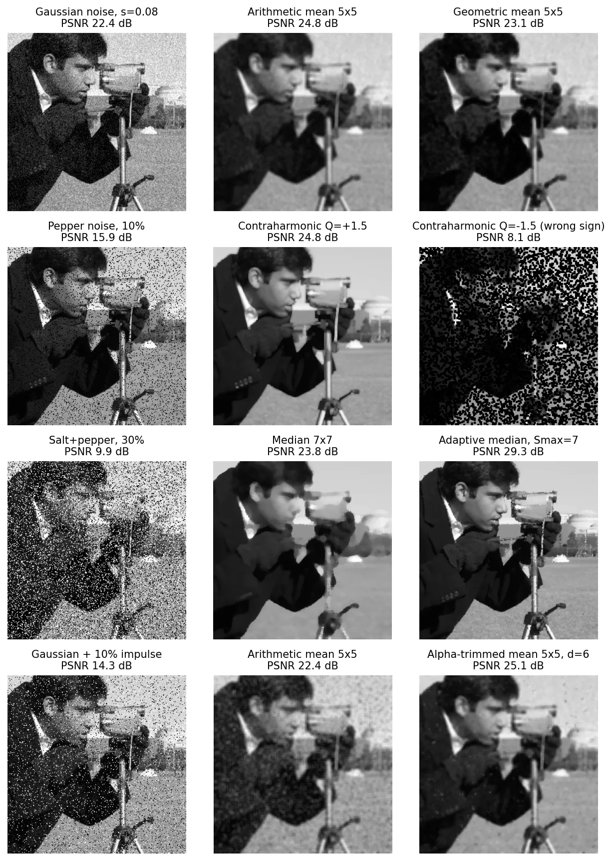

Periodic noise reduction using frequency-domain filtering

In plain words: periodic noise is a few pure “tones” hidden in the image. In the spectrum they show up as bright dots, so we cut out exactly those dots and leave everything else.

Notch reject and notch pass filters

A notch filter rejects (or passes) frequencies in small neighbourhoods around chosen centres. Because the DFT of a real image is conjugate-symmetric, notches always come in pairs, at $(u_k, v_k)$ and $(-u_k, -v_k)$ relative to the centre of the spectrum. A notch reject filter with $Q$ notch pairs is a product of highpass filters whose centres have been moved to the notches:

$$H_{NR}(u, v) = \prod_{k=1}^{Q} H_k(u, v)\, H_{-k}(u, v),$$

where $H_k$ and $H_{-k}$ are highpass filters (ideal, Butterworth or Gaussian, as in Chapter 4) centred at $(u_k, v_k)$ and $(-u_k, -v_k)$. For example, a Gaussian notch uses $H_k = 1 - e^{-D_k^2 / 2 D_0^2}$, with $D_k(u,v)$ the distance from $(u,v)$ to $(u_k, v_k)$ and $D_0$ the notch radius. The matching notch pass filter is

$$H_{NP}(u, v) = 1 - H_{NR}(u, v).$$

The notch pass filter is useful on its own: applying it to $G$ and transforming back gives an image of the interference pattern alone. Notch filters of other shapes (for instance a thin line along an axis) remove scan-line patterns.

import numpy as np
from skimage import data, img_as_float

f = img_as_float(data.moon())
M, N = f.shape
y, x = np.mgrid[:M, :N]
g = f + 0.2 * np.sin(2 * np.pi * (40 * y / M + 25 * x / N))    # periodic interference

G = np.fft.fftshift(np.fft.fft2(g))
U, V = np.mgrid[-M // 2:M // 2, -N // 2:N // 2]
H = np.ones((M, N))
for u0, v0 in [(40, 25), (-40, -25)]:                         # a spike and its mirror
    D2 = (U - u0) ** 2 + (V - v0) ** 2
    H *= 1 - np.exp(-D2 / (2 * 3.0 ** 2))                     # Gaussian notch, radius ~3
f_hat = np.real(np.fft.ifft2(np.fft.ifftshift(H * G)))

Optimum notch filtering

When there are several interference components, or they are not sharp spikes, a plain notch filter either removes too little or cuts away real image content. Optimum notch filtering works in two steps. First, isolate an estimate of the interference with a notch pass filter:

$$\hat\eta(x, y) = \mathfrak{F}^{-1}\{H_{NP}(u, v)\, G(u, v)\},$$

where $\mathfrak{F}^{-1}$ is the inverse DFT. Second, subtract a weighted version of it, with a weight that varies across the image:

$$\hat f(x, y) = g(x, y) - w(x, y)\, \hat\eta(x, y).$$

The weight $w(x,y)$ is chosen to make $\hat f$ as smooth as possible: it minimizes the variance of $\hat f$ inside a small window around each pixel. Setting the derivative of that local variance with respect to $w$ to zero gives

$$w(x, y) = \frac{\overline{g\hat\eta} - \bar g\, \bar{\hat\eta}}{\overline{\hat\eta^2} - \bar{\hat\eta}^2},$$

where each bar is a local average over the window. The numerator is the local covariance of $g$ and $\hat\eta$; the denominator is the local variance of $\hat\eta$. So the method subtracts more interference where the image and the estimated pattern move together, and less where they do not.

Linear, position-invariant degradations

In plain words: we assume the blur is “fair”. Twice as much light gives twice as much blurred light, and the blur is the same in the top-left corner as in the bottom-right.

Write the degradation (without noise) as an operator $\mathcal{H}$, so $g = \mathcal{H}[f] + \eta$. $\mathcal{H}$ is linear if

$$\mathcal{H}[a f_1 + b f_2] = a\,\mathcal{H}[f_1] + b\,\mathcal{H}[f_2]$$

for any images $f_1, f_2$ and constants $a, b$. It is position invariant if shifting the input only shifts the output:

$$\mathcal{H}[f(x - \alpha, y - \beta)] = g(x - \alpha, y - \beta)$$

for any shift $(\alpha, \beta)$. For such an operator, write $f$ as a sum of shifted impulses. Linearity lets us apply $\mathcal{H}$ to each impulse separately, and position invariance says every impulse produces the same response $h$, just shifted. Summing these responses is exactly convolution:

$$g(x, y) = \int_{-\infty}^{\infty} \int_{-\infty}^{\infty} f(\alpha, \beta)\, h(x - \alpha, y - \beta)\, d\alpha\, d\beta + \eta(x, y) = (h \star f)(x, y) + \eta(x, y).$$

Here $h(x, y) = \mathcal{H}[\delta(x, y)]$ is the impulse response, which in optics is the point spread function: the image of a single point of light. This is why restoring a blurred image is often called deconvolution, and why the filters below are built in the frequency domain.

Many real degradations are only approximately LPI. A lens may blur more at the image corners, and an object moving in front of a still background blurs differently from the background. Space-variant restoration exists, but it is far more expensive; the common workaround is to split the image into tiles that are roughly LPI.

Estimating the degradation function

In plain words: before we can undo the blur, we must know the blur. We can look for clues in the picture, test the camera ourselves, or derive the blur from physics.

By observation

Find a small region of the blurred image $g_s(x,y)$ with simple, strong structure, such as an edge or a small bright object, where signal is much stronger than noise. Build by hand (or by sharpening and judgment) an estimate $\hat f_s(x,y)$ of what that region should look like. Then

$$H_s(u, v) = \frac{G_s(u, v)}{\hat F_s(u, v)}$$

estimates the OTF from that small region. If the blur is position invariant, $H_s$ tells us the shape of $H$ for the whole image, scaled up to full size. This is laborious and used mainly when the image is all there is, for example a historical photograph.

By experimentation

If you have the same (or an equivalent) imaging system, image a tiny bright dot under the same settings. A small enough dot approximates an impulse of strength $A$, whose Fourier transform is the constant $A$. The observed image of the dot then gives the OTF directly:

$$H(u, v) = \frac{G(u, v)}{A}.$$

Microscopists do exactly this with sub-resolution fluorescent beads.

By mathematical modeling

Sometimes physics gives the answer. Two classic models are used throughout this chapter.

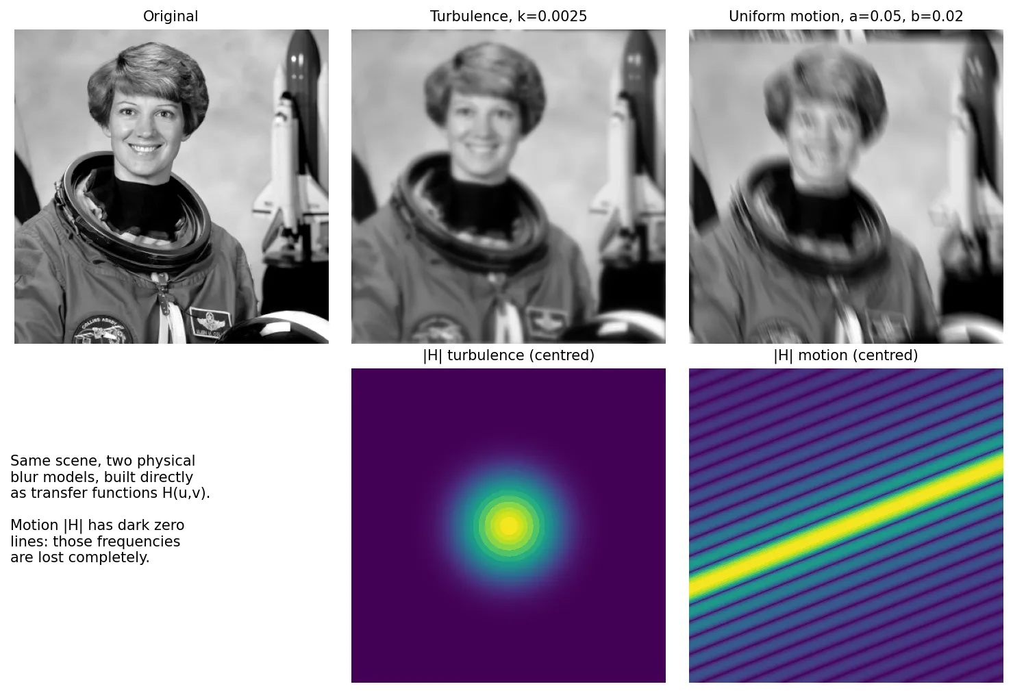
Atmospheric turbulence. Long-exposure imaging through turbulent air is often modelled by

$$H(u, v) = e^{-k\,(u^2 + v^2)^{5/6}},$$

where $k$ is a constant that grows with the strength of the turbulence. Apart from the $5/6$ power it looks like a Gaussian lowpass filter, and it never reaches exactly zero.

Uniform linear motion blur. Suppose the image $f$ moves during an exposure of length $T$, with displacement $x_0(t)$ and $y_0(t)$. The sensor integrates every position:

$$g(x, y) = \int_0^T f\bigl(x - x_0(t),\, y - y_0(t)\bigr)\, dt.$$

Taking the Fourier transform and using the shift property gives

$$H(u, v) = \int_0^T e^{-j 2\pi [u\, x_0(t) + v\, y_0(t)]}\, dt.$$

For uniform motion, $x_0(t) = a t / T$ and $y_0(t) = b t / T$, where $a$ and $b$ are the total displacements in $x$ and $y$. The integral evaluates to

$$H(u, v) = \frac{T}{\pi(u a + v b)}\, \sin\bigl[\pi(u a + v b)\bigr]\, e^{-j\pi(u a + v b)}.$$

This is a sinc function along the direction of motion, with a linear phase term. Crucially, it is exactly zero wherever $u a + v b$ is a non-zero integer, so whole lines of frequencies are destroyed (Figure 5.4).

import numpy as np

def freq_grid(shape):
    u = np.fft.fftfreq(shape[0]) * shape[0]            # 0, 1, ..., -1 (un-centred)
    v = np.fft.fftfreq(shape[1]) * shape[1]
    return np.meshgrid(u, v, indexing="ij")

def motion_blur_otf(shape, a, b, T=1.0):
    U, V = freq_grid(shape)
    s = np.pi * (U * a + V * b)
    return T * np.sinc(s / np.pi) * np.exp(-1j * s)    # np.sinc(x) = sin(pi x) / (pi x)

def turbulence_otf(shape, k):
    U, V = freq_grid(shape)
    return np.exp(-k * (U ** 2 + V ** 2) ** (5 / 6))

Inverse filtering

In plain words: if the blur multiplied each frequency by $H$, just divide by $H$. It is the obvious idea, and it fails spectacularly as soon as there is noise.

The direct inverse filter estimates

$$\hat F(u, v) = \frac{G(u, v)}{H(u, v)}.$$

Substituting $G = HF + N$ shows the problem:

$$\hat F(u, v) = F(u, v) + \frac{N(u, v)}{H(u, v)}.$$

Even if we knew $H$ perfectly, we cannot recover $F$ exactly, because $N$ is unknown. Worse, blur makes $|H|$ tiny at high frequencies (or exactly zero, as for motion), while noise is roughly white and keeps its power there. So $N/H$ becomes enormous and swamps the image. In Figure 5.5, the full inverse filter turns both images into pure noise, even though the noise standard deviation is only 0.3% and 1% of the intensity range.

A partial fix is to apply the inverse only near the origin of the spectrum, where $|H|$ is large, for instance by multiplying $\hat F$ by a sharp Butterworth lowpass of radius $D_0$. This works for the turbulence blur, whose $H$ shrinks smoothly. It does not work well for motion blur, because the zero lines of $H$ cross the low frequencies too. The radius must be tuned by hand. We need a method that decides automatically how much to trust each frequency.

Minimum mean square error (Wiener) filtering

In plain words: at every frequency, ask “is there more picture or more noise here?” Where the picture dominates, undo the blur. Where noise dominates, hold back.

The Wiener filter treats both the image and the noise as random fields and seeks the estimate that minimizes the mean squared error

$$e^2 = E\bigl\{(f - \hat f)^2\bigr\},$$

where $E\{\cdot\}$ is the expected value. Assume the noise and the image are uncorrelated, that one of them has zero mean, and that $\hat f$ is a linear function of $g$.

Derivation sketch. For stationary signals the DFT decouples the frequencies, so we can choose a gain $W(u,v)$ for each frequency separately and set $\hat F = W G$. The expected error at one frequency is

$$E\bigl\{|F - W G|^2\bigr\} = S_f - W H S_f - W^* H^* S_f + |W|^2\bigl(|H|^2 S_f + S_\eta\bigr),$$

where $S_f(u,v) = E\{|F(u,v)|^2\}$ is the power spectrum of the image, $S_\eta(u,v) = E\{|N(u,v)|^2\}$ is the power spectrum of the noise, $^*$ denotes complex conjugation, and the cross terms with $N$ vanish because image and noise are uncorrelated. This is a quadratic in $W$; setting its derivative with respect to $W^*$ to zero gives

$$W(u, v) = \frac{H^*(u, v)\, S_f(u, v)}{|H(u, v)|^2\, S_f(u, v) + S_\eta(u, v)}.$$

Dividing top and bottom by $S_f$ gives the form that is easiest to read:

$$\hat F(u, v) = \left[\frac{1}{H(u, v)}\, \frac{|H(u, v)|^2}{|H(u, v)|^2 + S_\eta(u, v) / S_f(u, v)}\right] G(u, v).$$

The first factor is the inverse filter. The second factor is between 0 and 1. Where the signal is strong compared to the noise, $S_\eta/S_f \approx 0$, the factor is close to 1 and the filter acts as an inverse filter. Where noise dominates, the factor shrinks toward 0 and switches that frequency off. If $H = 0$ at some frequency, the bracket is $0$ there (write it as $H^*/(|H|^2 + S_\eta/S_f)$ to avoid dividing by zero). With no noise, $S_\eta = 0$, the Wiener filter is the inverse filter.

The constant-$K$ approximation

We rarely know $S_f$, the power spectrum of the image we are trying to find. The common shortcut replaces the ratio $S_\eta / S_f$ by a single constant $K$:

$$\hat F(u, v) = \frac{H^*(u, v)}{|H(u, v)|^2 + K}\, G(u, v).$$

$K$ is tuned by eye or chosen to optimize a quality measure. A useful starting point is the ratio of the noise variance to the image variance, which is the inverse of the signal-to-noise ratio. A small $K$ gives a sharper but noisier result; a large $K$ a smoother one.

import numpy as np
from skimage import data, img_as_float

rng = np.random.default_rng(0)
f = img_as_float(data.camera())[::2, ::2]                # 256 x 256
H = motion_blur_otf(f.shape, a=0.1, b=0.1)               # from the snippet above
g = np.real(np.fft.ifft2(H * np.fft.fft2(f))) + rng.normal(0, 0.01, f.shape)
G = np.fft.fft2(g)

def wiener(G, H, K):
    return np.real(np.fft.ifft2(np.conj(H) / (np.abs(H) ** 2 + K) * G))

f_hat = wiener(G, H, K=0.01)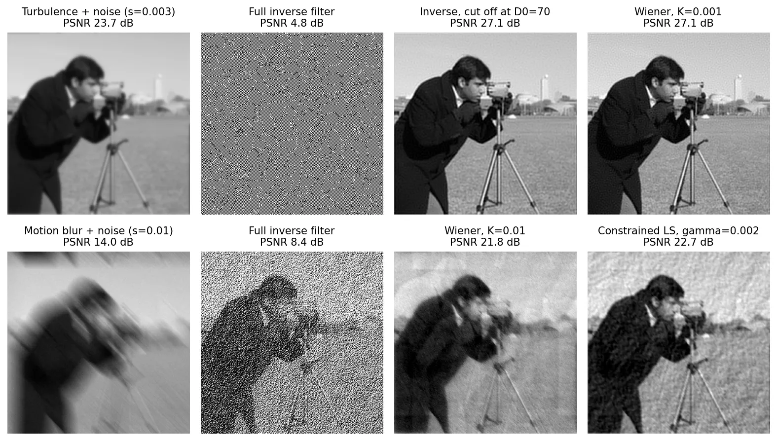

Drag the slider to compare the motion-blurred, noisy image with its Wiener restoration (full 512 × 512 version, $K = 0.01$).

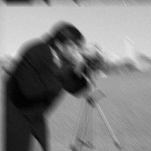
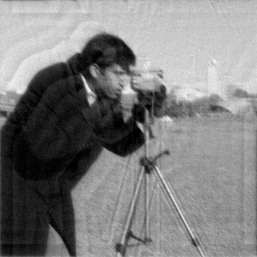Motion blur + noiseWiener, K=0.01

Constrained least squares filtering

In plain words: among all images that would explain what we observed, up to the expected amount of noise, pick the smoothest one.

The Wiener filter needs power spectra, or a constant $K$ with no clear meaning. Constrained least squares (CLS) filtering needs only the noise mean and variance [3]. In matrix-vector form, stack the pixels into vectors so that the model is

$$\mathbf{g} = \mathbf{H}\mathbf{f} + \boldsymbol{\eta},$$

where $\mathbf{g}, \mathbf{f}, \boldsymbol{\eta}$ are $MN \times 1$ vectors and $\mathbf{H}$ is the $MN \times MN$ blur matrix. These matrices are far too large to invert directly, but because $\mathbf{H}$ represents a circular convolution it is diagonalized by the DFT, which is what makes a closed-form frequency-domain answer possible.

Inverse problems like this are ill-conditioned: tiny changes in $\mathbf g$ cause huge changes in the solution. CLS fixes this by preferring smooth solutions. It measures roughness with the Laplacian $\nabla^2$ and solves

$$\min_{\hat{\mathbf f}}\ C = \sum_{x=0}^{M-1} \sum_{y=0}^{N-1} \bigl[\nabla^2 \hat f(x, y)\bigr]^2 \quad \text{subject to} \quad \|\mathbf{g} - \mathbf{H}\hat{\mathbf{f}}\|^2 = \|\boldsymbol{\eta}\|^2,$$

where $\|\cdot\|$ is the Euclidean norm. The constraint says: the residual should be exactly as large as the noise, no more (we would be ignoring data) and no less (we would be fitting noise). The solution, found with a Lagrange multiplier, is

$$\hat F(u, v) = \left[\frac{H^*(u, v)}{|H(u, v)|^2 + \gamma\, |P(u, v)|^2}\right] G(u, v),$$

where $\gamma \ge 0$ is the multiplier and $P(u, v)$ is the DFT of the Laplacian kernel

$$p(x, y) = \begin{bmatrix} 0 & -1 & 0 \\ -1 & 4 & -1 \\ 0 & -1 & 0 \end{bmatrix},$$

zero-padded to $M \times N$ before transforming. With $\gamma = 0$ we are back at the inverse filter. Compare with the constant-$K$ Wiener filter: CLS replaces the flat $K$ with $\gamma |P|^2$, which is small at low frequencies and large at high frequencies, so it holds back exactly where noise tends to dominate.

Choosing $\gamma$

$\gamma$ is not a free knob: it must make the constraint hold. Define the residual $\mathbf{r} = \mathbf{g} - \mathbf{H}\hat{\mathbf{f}}$ and $\phi(\gamma) = \|\mathbf{r}\|^2$. One can show that $\phi$ is monotonically increasing in $\gamma$. So:

1. Start from some $\gamma$.
2. Compute $\hat F$ and the residual $\|\mathbf{r}\|^2$ (both cheap with the FFT).
3. If $\|\mathbf{r}\|^2 < \|\boldsymbol{\eta}\|^2 - a$, increase $\gamma$; if $\|\mathbf{r}\|^2 > \|\boldsymbol{\eta}\|^2 + a$, decrease it; otherwise stop. Here $a$ is a small tolerance.

The target needs only the noise statistics: $\|\boldsymbol{\eta}\|^2 = MN\,(\sigma_\eta^2 + \bar\eta^2)$, where $\sigma_\eta^2$ and $\bar\eta$ are the noise variance and mean, which we already know how to estimate from a flat patch.

def cls(G, H, gamma):
    p = np.zeros(H.shape)
    p[[0, 0, 0, 1, -1], [0, 1, -1, 0, 0]] = [4, -1, -1, -1, -1]   # Laplacian centred at (0, 0)
    P = np.fft.fft2(p)
    return np.real(np.fft.ifft2(np.conj(H) / (np.abs(H) ** 2 + gamma * np.abs(P) ** 2) * G))

f_hat = cls(G, H, gamma=0.002)

Which is better, Wiener or CLS? Neither in general. Wiener is optimal on average over an ensemble of images that share the assumed power spectra. CLS is tailored to the one image at hand and can give a better result for that image when the noise statistics are known. When $K$ or $\gamma$ is hand-tuned, as is common, the two often look similar (Figure 5.5).

Geometric mean filter

In plain words: a single dial that slides between “undo the blur fully” and “play it safe against noise”.

The geometric mean filter combines the inverse and the (parametric) Wiener filter:

$$\hat F(u, v) = \left[\frac{H^*(u, v)}{|H(u, v)|^2}\right]^{\alpha} \left[\frac{H^*(u, v)}{|H(u, v)|^2 + \beta\, \dfrac{S_\eta(u, v)}{S_f(u, v)}}\right]^{1 - \alpha} G(u, v),$$

where $\alpha$ and $\beta$ are non-negative real constants. Special cases:

• $\alpha = 1$: the inverse filter.
• $\alpha = 0$: the parametric Wiener filter; with $\beta = 1$ it is the standard Wiener filter.
• $\alpha = 1/2$, $\beta = 1$: the geometric mean of the inverse and Wiener filters, which gives this family its name. It is also called the spectrum equalization filter: you can check that the expected power spectrum of its output, $|W|^2 (|H|^2 S_f + S_\eta)$, is then exactly $S_f$, the power spectrum of the original image.

With $\beta > 1$ the filter is more cautious than Wiener; with $\beta < 1$ it is bolder.

def geometric_mean_filter(G, H, alpha, beta, K):
    """K stands in for S_eta / S_f, as in the constant-K Wiener filter."""
    H2 = np.abs(H) ** 2
    inv = np.conj(H) / np.maximum(H2, 1e-12)
    wie = np.conj(H) / (H2 + beta * K)
    # Both factors have the phase of conj(H): combine magnitudes, keep that phase.
    return np.real(np.fft.ifft2(np.abs(inv) ** alpha * np.abs(wie) ** (1 - alpha)
                                * np.exp(1j * np.angle(wie)) * G))

Image reconstruction from projections

In plain words: shine X-rays through a body from many angles. Each angle gives a “shadow” that only tells how much stuff the ray passed through in total. Put enough shadows together, cleverly, and you can rebuild the inside slice.

Principles of computed tomography (CT)

In X-ray CT, a source and a row of detectors rotate around the patient. For each angle, every detector measures how much the X-ray beam was attenuated along its straight path. Attenuation along a ray adds up (the log of the intensity ratio is the line integral of the attenuation coefficient), so each measurement is a line integral of the unknown slice $f(x,y)$. The set of measurements for one angle is a projection. CT scanners evolved from a single source-detector pair that translates and rotates (parallel beams), to fan beams with many detectors, to helical and cone-beam geometries that acquire whole volumes; the reconstruction mathematics below is the core of all of them [4].

Projections and the Radon transform

Describe a straight line in normal form, $x\cos\theta + y\sin\theta = \rho$, where $\rho$ is its distance from the origin and $\theta$ the angle of its normal. The line integral of $f$ along that line is

$$g(\rho, \theta) = \int_{-\infty}^{\infty}\int_{-\infty}^{\infty} f(x, y)\, \delta(x\cos\theta + y\sin\theta - \rho)\, dx\, dy,$$

where $\delta$ is the Dirac impulse, which keeps only the points on the line. As a function of $(\rho, \theta)$, $g$ is the Radon transform of $f$. Displayed as an image with $\theta$ on one axis and $\rho$ on the other it is called a sinogram: a single point in the slice traces a sinusoid, $\rho = x_0\cos\theta + y_0\sin\theta$.

The simplest way to go back is backprojection: smear each projection back across the image along the direction it came from, and add up the smears over all angles:

$$f_{\theta}(x, y) = g(x\cos\theta + y\sin\theta,\ \theta), \qquad f_{BP}(x, y) = \int_0^{\pi} f_{\theta}(x, y)\, d\theta.$$

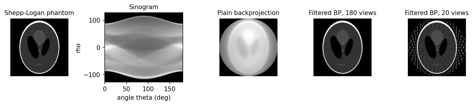
This puts mass in the right places, but also everywhere along each ray, so the result is a heavily blurred version of $f$ (Figure 5.6, third panel). The blur is not random: it is a convolution with $1/r$, where $r$ is the distance from the centre. The Fourier-slice theorem shows how to remove it.

The Fourier-slice theorem

Let $G(\omega, \theta)$ be the 1-D Fourier transform of the projection $g(\rho, \theta)$ with respect to $\rho$, at a fixed angle $\theta$:

$$G(\omega, \theta) = \int_{-\infty}^{\infty} g(\rho, \theta)\, e^{-j2\pi\omega\rho}\, d\rho.$$

The Fourier-slice theorem (also called the projection-slice theorem) states that

$$G(\omega, \theta) = F(\omega\cos\theta,\ \omega\sin\theta),$$

where $F(u,v)$ is the 2-D Fourier transform of $f$. In words: the 1-D transform of a projection equals a radial slice, through the origin at angle $\theta$, of the 2-D transform of the object. The proof is short: substitute the Radon integral into $G$, integrate out the delta, and the exponent becomes $-j2\pi\omega(x\cos\theta + y\sin\theta)$, which is exactly the 2-D transform evaluated at $(u, v) = (\omega\cos\theta, \omega\sin\theta)$.

So in principle, projections from all angles fill the 2-D spectrum, slice by slice, and a 2-D inverse transform returns $f$. In practice the slices sample the spectrum on a polar grid, densely near the origin and sparsely far from it, and interpolating onto a Cartesian grid is error-prone. That uneven sampling is also the reason plain backprojection blurs: it over-weights low frequencies.

Filtered backprojection with parallel beams

Write the 2-D inverse Fourier transform in polar coordinates $u = \omega\cos\theta$, $v = \omega\sin\theta$. The area element $du\,dv$ becomes $|\omega|\, d\omega\, d\theta$, and with the Fourier-slice theorem:

$$f(x, y) = \int_0^{\pi} \left[\int_{-\infty}^{\infty} |\omega|\, G(\omega, \theta)\, e^{j2\pi\omega\rho}\, d\omega\right]_{\rho = x\cos\theta + y\sin\theta} d\theta.$$

Read it from the inside out. For each angle, multiply the 1-D spectrum of the projection by $|\omega|$, the ramp filter, and transform back. Then backproject the filtered projection and sum over angles. This is filtered backprojection (FBP). The ramp exactly cancels the $1/r$ blur of plain backprojection.

The ramp grows without bound, so it amplifies high-frequency noise and is not integrable. In practice it is band-limited and multiplied by a smooth window, for example a Hamming window $h(\omega) = c + (1 - c)\cos(2\pi\omega / W)$ inside the band $|\omega| \le W/2$ and $0$ outside, where $W$ is the bandwidth and $c = 0.54$. The window equals 1 at $\omega = 0$ and falls to $2c - 1 = 0.08$ at the band edge. The window trades a little sharpness for much less ringing and noise. A filter introduced alongside the famous head phantom of Shepp and Logan [5] is still one of the standard options. The number of views matters as well: with too few angles, FBP produces streaks (Figure 5.6, last panel).

import numpy as np
from skimage.data import shepp_logan_phantom
from skimage.transform import radon, iradon, rescale

f = rescale(shepp_logan_phantom(), 0.64)                 # 256 x 256
theta = np.linspace(0.0, 180.0, 180, endpoint=False)     # projection angles in degrees
sinogram = radon(f, theta=theta)                         # shape: (detector bins, angles)
backproj = iradon(sinogram, theta=theta, filter_name=None)    # blurry, no filter
fbp = iradon(sinogram, theta=theta, filter_name="ramp")       # filtered backprojection
rmse = np.sqrt(np.mean((fbp - f) ** 2))

iradon also accepts "shepp-logan", "cosine", "hamming" and "hann" windows, and skimage.transform.iradon_sart gives an iterative alternative [6].

Fan-beam filtered backprojection

Modern scanners use a fan beam: one point source and a curved or flat detector array, so rays in one view are not parallel. Each fan-beam ray is still some line $(\rho, \theta)$, so there are two routes. Rebinning sorts fan-beam rays from many views into sets of parallel rays and then applies parallel FBP. Direct fan-beam FBP changes variables in the FBP integral: projections are first multiplied by a cosine weight that depends on the ray’s angle within the fan, then filtered with a modified ramp, and finally backprojected with a weight that depends on the distance from the source. The structure, weight-filter-backproject, is the same [4].

Modern view

The tools of this chapter are not museum pieces. The model $g = h \star f + \eta$ is still how the field states its problems, and Wiener-like steps still sit inside modern networks. What deep learning changed is the prior: instead of assuming “the image is smooth” (CLS) or “the image has power spectrum $S_f$” (Wiener), we now learn what clean images look like from data. For a broad tour of deep image restoration beyond this chapter (super-resolution, dehazing, deraining, low-light, all-in-one restoration and diffusion priors), see the site owner’s post Low-Level Vision Task — Image Restoration 簡介 (in Traditional Chinese). The surveys below focus on the three topics of this chapter: denoising, deblurring and CT reconstruction.

Denoising: from patches to networks

Two classical methods marked the peak of hand-designed denoising. Non-local means (NLM) [7] replaces each pixel by a weighted average of pixels whose surrounding patches look similar, wherever they are in the image. It is the adaptive filter idea taken much further: the “neighbourhood” is defined by similarity, not distance. BM3D [8] groups similar patches into a 3-D stack, filters the stack jointly in a transform domain, and then applies a Wiener-type filter in a second stage, using the first-stage result as its estimate of $S_f$. It was the standard baseline for about a decade.

DnCNN [9] showed that a plain deep convolutional network trained with residual learning (predicting the noise rather than the clean image) and batch normalization beats BM3D on Gaussian noise, and that one model can handle unknown noise levels.

• Tian et al., “Deep learning on image denoising: An overview” (2020) [10]. Organises CNN denoisers into four groups: additive white Gaussian noise, real (camera) noise, blind denoising (unknown noise), and hybrid cases with blur or low resolution. Takeaway (our reading): the taxonomy itself is organised by noise type, with real camera noise and unknown noise levels as separate categories from synthetic Gaussian noise. The noise model from this chapter, and how realistic it is, stays central in deep denoising.
• Elad, Kawar and Vaksman, “Image Denoising: The Deep Learning Revolution and Beyond” (2023) [11]. Traces the history from classical priors to deep denoisers, then argues that denoisers matter beyond denoising. A good denoiser can serve as the prior inside a solver for other inverse problems, and it is the engine of diffusion-based image generation. Takeaway: the classic “noise only” problem of this chapter has become a building block for nearly everything else.

Deblurring and general inverse problems

• Zhang et al., “Deep Image Deblurring: A Survey” (IJCV 2022) [12]. Covers causes of blur, datasets and metrics, then a taxonomy of CNN-based non-blind and blind deblurring by architecture and loss, plus specialised domains (faces, text, stereo). Takeaway: non-blind deblurring (known $h$, as in this chapter) is largely about suppressing the noise amplification and ringing we saw with the inverse filter, while blind deblurring must estimate $h$ too, and that remains the harder problem.
• Ongie et al., “Deep Learning Techniques for Inverse Problems in Imaging” (2020) [13]. Gives a taxonomy for any $\mathbf g = \mathbf{H}\mathbf f + \boldsymbol\eta$ problem: is the forward model $\mathbf H$ known at training time, only at test time, or not at all, and is training supervised or unsupervised? Takeaway (our reading): how much you know about $\mathbf H$ is the first design decision, and the survey also discusses failure modes of the resulting methods. Knowing $\mathbf H$, as in this chapter, opens options that a purely end-to-end network ignores.
• Kamilov, Bouman, Buzzard and Wohlberg, “Plug-and-Play Methods for Integrating Physical and Learned Models in Computational Imaging” (2023) [14]. Reviews plug-and-play (PnP) priors: iterative algorithms that alternate between a step enforcing the physics ($\mathbf g \approx \mathbf H \mathbf f$) and a step that calls a denoiser, which stands in for the prior. Takeaway: the forward model and the learned prior can be developed separately and combined at run time. DPIR [15] is a widely used example that plugs a deep CNN denoiser into half-quadratic splitting for deblurring, super-resolution and demosaicing.

The connection to this chapter is direct. For a blur $H$, the physics step of such a splitting method asks for $\hat F$ minimizing $|G - HF|^2 + \mu|F - Z|^2$ at each frequency, where $Z$ is the current denoised estimate and $\mu$ a penalty weight. Its solution is $\hat F = (H^* G + \mu Z) / (|H|^2 + \mu)$, which is a constant-$K$ Wiener filter pulled toward $Z$ instead of toward zero.

CT reconstruction: learned and unrolled

FBP is fast and exact for complete, low-noise data. It struggles when data are reduced to lower the radiation dose, either fewer views (streaks, Figure 5.6) or fewer photons per view (noise). Classical answers are iterative methods with hand-made priors such as total variation. Deep learning offers three main patterns:

• Post-processing: run FBP, then a CNN removes the artifacts. FBPConvNet [16] does exactly this with a CNN and reports better quality than total-variation reconstruction on sparse-view CT at a fraction of the run time.
• Unrolled (learned iterative) reconstruction: take an iterative algorithm, fix its number of iterations, and replace parts of each iteration with small networks, trained end to end. Learned Primal-Dual [17] unrolls a primal-dual algorithm, keeping the forward projector and backprojector inside each iteration. Monga, Li and Eldar, “Algorithm Unrolling” (2019) [18] surveys this design pattern across signal and image processing. Takeaway: because each layer mirrors an algorithm step, unrolled networks are more interpretable and more efficient than generic networks.
• Wang, Ye and De Man, “Deep learning for tomographic image reconstruction” (2020) [19] reviews the whole landscape for CT and other tomographic modalities: image-domain, sensor-domain and hybrid networks, physics-informed designs, and the open issues of data availability, robustness and clinical validation.

What did not change: the Radon transform and the Fourier-slice theorem define the forward model that every one of these methods uses, and FBP remains the default in clinical scanners and the input or starting point of many learned methods. Learned methods also bring a new risk that this chapter’s linear filters do not have: a network can produce plausible structure that is not in the data. That is why validation on real, out-of-distribution scans matters in medical use.

Key takeaways

• Restoration is objective: model the degradation as $g = h \star f + \eta$ (or $G = HF + N$), then invert that model.
• Identify noise from the histogram of a flat patch; estimate its mean and variance from the same patch.
• Match the spatial filter to the noise: means for Gaussian-like noise, contraharmonic with the right sign of $Q$ for one-sided impulses, median and adaptive median for salt-and-pepper, alpha-trimmed for mixtures.
• Periodic noise is a few spikes in the spectrum; notch filters remove it, and optimum notch filtering adapts the subtraction locally.
• The inverse filter $G/H$ amplifies noise wherever $|H|$ is small. Wiener, constrained least squares and geometric mean filters all add a term to the denominator that holds back those frequencies.
• CT measures line integrals (the Radon transform). By the Fourier-slice theorem, each projection gives one slice of the 2-D spectrum, and filtered backprojection (ramp filter, then backproject) reconstructs the image.
• Deep learning replaced hand-made priors with learned ones, but the best methods still keep the forward model inside (plug-and-play, unrolled networks).

Exercises

1. A dark-field microscope image has a background region whose histogram is one-sided, starting sharply at 12 and with a long right tail; its mean is 20 and its variance is 64 (gray levels). Which PDF from this chapter would you try first, and what are its parameters?

Hint

A sharp start and a long tail point to the exponential, Rayleigh or Erlang family. Try an exponential shifted to start at 12: it needs $1/a = 20 - 12 = 8$ and $1/a^2 = 64$, and both hold with $a = 1/8$. A Rayleigh fit is inconsistent: $b(4 - \pi)/4 = 64$ gives $b \approx 298$, so its start would be $20 - \sqrt{\pi b/4} \approx 4.7$, not 12.

2. An image is corrupted only by salt noise. Without testing, predict what happens with (a) a max filter, (b) a min filter, (c) a contraharmonic filter with $Q = 2$, (d) with $Q = -2$. Then verify with the code in this chapter.

Hint

Salt pixels are the largest values in their windows. The max filter spreads them (worse), the min filter removes them (but darkens and erodes bright detail). Positive $Q$ weights large values more, so $Q = 2$ makes salt worse; $Q = -2$ removes it.

3. Show that the Wiener filter with constant $K$ reduces to the inverse filter when $K = 0$, and that for a frequency where $|H|^2 \ll K$ the output is approximately $(H^*/K)\,G$. What does this say about how Wiener filtering treats frequencies the blur destroyed?

Hint

When $|H|^2 \ll K$ the denominator is about $K$. The output is then small, proportional to $|H|$, so the filter does not try to recover those frequencies. It gives up on them gracefully instead of amplifying noise.

4. A $256 \times 256$ image is blurred by uniform motion of 8 pixels along $x$ and none along $y$. Frequencies are integers (cycles per image), as in the code above. Using the motion blur OTF, find all frequencies $(u, v)$ with $H(u,v) = 0$. Explain why no linear filter can restore detail at those frequencies, and what that looks like in the restored image.

Hint

With $u$ in cycles per image, $a$ is the blur length as a fraction of the image size, so $a = 8/256 = 1/32$ and $b = 0$. Then $H = 0$ when $u/32$ is a non-zero integer: $u = \pm 32, \pm 64, \pm 96, \pm 128$, for every $v$. Since $G = HF + N$ has no $F$ content there, any linear filter outputs only noise (or zero) at those frequencies. Expect faint ringing at that spatial period along $x$.

5. In the CT code above, reconstruct with 180, 60, 20 and 10 views, and with the ramp and hann filters. Plot RMSE versus number of views. Then add Gaussian noise to the sinogram and repeat. When does the smoother hann filter win?

Hint

Without noise, ramp should win at many views. As noise grows, the ramp amplifies it at high frequencies and hann (which rolls off there) wins, which is the same trade-off as inverse filter versus Wiener filter.

6. Derive the per-frequency solution $\hat F = (H^* G + \mu Z)/(|H|^2 + \mu)$ of $\min_F |G - HF|^2 + \mu|F - Z|^2$. What filter from this chapter do you get when $Z = 0$?

Hint

Differentiate with respect to $F^*$: $-H^*(G - HF) + \mu(F - Z) = 0$. With $Z = 0$ it is the Wiener filter with constant $K = \mu$.

References

1. R. C. Gonzalez and R. E. Woods, Digital Image Processing, 4th ed., Pearson, 2018, Ch. 5. publisher page
2. H. Hwang and R. A. Haddad, “Adaptive median filters: new algorithms and results,” IEEE Transactions on Image Processing, vol. 4, no. 4, pp. 499–502, 1995. DOI
3. B. R. Hunt, “The application of constrained least squares estimation to image restoration by digital computer,” IEEE Transactions on Computers, vol. C-22, no. 9, pp. 805–812, 1973. DOI
4. A. C. Kak and M. Slaney, Principles of Computerized Tomographic Imaging, IEEE Press, 1988 (SIAM reprint 2001). free online edition
5. L. A. Shepp and B. F. Logan, “The Fourier reconstruction of a head section,” IEEE Transactions on Nuclear Science, vol. 21, no. 3, pp. 21–43, 1974. DOI
6. scikit-image developers, “Radon transform,” scikit-image documentation (gallery example). docs
7. A. Buades, B. Coll and J.-M. Morel, “A non-local algorithm for image denoising,” IEEE CVPR, vol. 2, pp. 60–65, 2005. DOI
8. K. Dabov, A. Foi, V. Katkovnik and K. Egiazarian, “Image denoising by sparse 3-D transform-domain collaborative filtering,” IEEE Transactions on Image Processing, vol. 16, no. 8, pp. 2080–2095, 2007. DOI
9. K. Zhang, W. Zuo, Y. Chen, D. Meng and L. Zhang, “Beyond a Gaussian denoiser: Residual learning of deep CNN for image denoising,” IEEE Transactions on Image Processing, vol. 26, no. 7, pp. 3142–3155, 2017. doi · arXiv
10. C. Tian, L. Fei, W. Zheng, Y. Xu, W. Zuo and C.-W. Lin, “Deep learning on image denoising: An overview,” Neural Networks, vol. 131, pp. 251–275, 2020. arXiv
11. M. Elad, B. Kawar and G. Vaksman, “Image denoising: The deep learning revolution and beyond — A survey paper,” SIAM Journal on Imaging Sciences, vol. 16, no. 3, pp. 1594–1654, 2023. arXiv
12. K. Zhang, W. Ren, W. Luo, W.-S. Lai, B. Stenger, M.-H. Yang and H. Li, “Deep image deblurring: A survey,” International Journal of Computer Vision, 2022. arXiv
13. G. Ongie, A. Jalal, C. A. Metzler, R. G. Baraniuk, A. G. Dimakis and R. Willett, “Deep learning techniques for inverse problems in imaging,” arXiv:2005.06001, 2020. arXiv
14. U. S. Kamilov, C. A. Bouman, G. T. Buzzard and B. Wohlberg, “Plug-and-play methods for integrating physical and learned models in computational imaging: Theory, algorithms, and applications,” IEEE Signal Processing Magazine, vol. 40, no. 1, pp. 85–97, 2023. arXiv
15. K. Zhang, Y. Li, W. Zuo, L. Zhang, L. Van Gool and R. Timofte, “Plug-and-play image restoration with deep denoiser prior,” IEEE Transactions on Pattern Analysis and Machine Intelligence, vol. 44, no. 10, pp. 6360–6376, 2022. arXiv
16. K. H. Jin, M. T. McCann, E. Froustey and M. Unser, “Deep convolutional neural network for inverse problems in imaging,” IEEE Transactions on Image Processing, vol. 26, no. 9, pp. 4509–4522, 2017. arXiv
17. J. Adler and O. Öktem, “Learned primal-dual reconstruction,” IEEE Transactions on Medical Imaging, 2018. arXiv
18. V. Monga, Y. Li and Y. C. Eldar, “Algorithm unrolling: Interpretable, efficient deep learning for signal and image processing,” arXiv:1912.10557, 2019. arXiv
19. G. Wang, J. C. Ye and B. De Man, “Deep learning for tomographic image reconstruction,” Nature Machine Intelligence, vol. 2, no. 12, pp. 737–748, 2020. DOI