Chapter 3 · Intensity Transformations and Spatial Filtering

What you’ll learn

• How a single curve $s = T(r)$ can brighten, darken, invert or stretch an image, and when to pick a log, gamma or piecewise-linear curve.
• Why histogram equalization works, derived step by step, and how histogram matching, CLAHE-style local methods and local statistics build on it.
• What linear spatial filtering is, how correlation differs from convolution, and why separable kernels are fast.
• How smoothing (lowpass) filters, including the nonlinear median filter, remove noise, and how derivative-based (highpass) filters sharpen.
• How to derive highpass, bandpass and bandreject kernels from a lowpass one, and how to chain several methods into one pipeline.

The big picture

This chapter is about improving an image without leaving the pixel grid. Every method here works on the pixel values directly, which is what “spatial domain” means. There are two families. Point operations change each pixel using only its own value. Neighborhood operations (spatial filters) change each pixel using the values around it.

Why it matters: these are the first tools anyone reaches for, in phone cameras, medical viewers, microscopes and as preprocessing for computer-vision models. They are also the conceptual ancestors of the convolutional layer. A CNN’s first layer is a bank of spatial filters, and many learned enhancement networks still output a curve or a filter, as we will see in the Modern view.

Background

Plain version. We write the output image as some operation applied to the input image. If the operation only looks at one pixel at a time, it is a lookup table. If it looks at a small window, it is a filter.

Precise version. Let $I(x, y)$ be the input image and $G(x, y)$ the output, with $x, y$ integer pixel coordinates (the same names as in the convolution tutorial). A spatial-domain process is

$$G(x, y) = T\big[I\big](x, y),$$

where $T$ is an operator defined over a neighborhood of $(x, y)$. The neighborhood is usually a small square or rectangle centered on $(x, y)$. The operator is applied at every location by moving the neighborhood’s center from pixel to pixel.

When the neighborhood is a single pixel ($1 \times 1$), $T$ depends only on the value at that pixel. We then call it an intensity transformation (also gray-level or point transformation) and write it with scalars:

$$s = T(r),$$

where $r$ is the input intensity at a pixel, $s$ is the output intensity at the same pixel, and both lie in $[0, L-1]$ for an image with $L$ intensity levels ($L = 256$ for 8-bit images). Because $r$ takes only $L$ values, any $T$ can be stored as a lookup table of length $L$, which is why point operations are extremely fast.

Basic intensity transformation functions

Plain version. Draw a curve from input brightness (horizontal axis) to output brightness (vertical axis). Where the curve is steep, nearby gray levels get pulled apart, so contrast increases. Where it is flat, they get squeezed together, so contrast drops.

The slope $T'(r)$ is the local contrast gain: a small difference $\Delta r$ between two neighboring pixels becomes roughly $T'(r)\,\Delta r$ after the transformation. Every curve below is a choice about where to spend that gain.

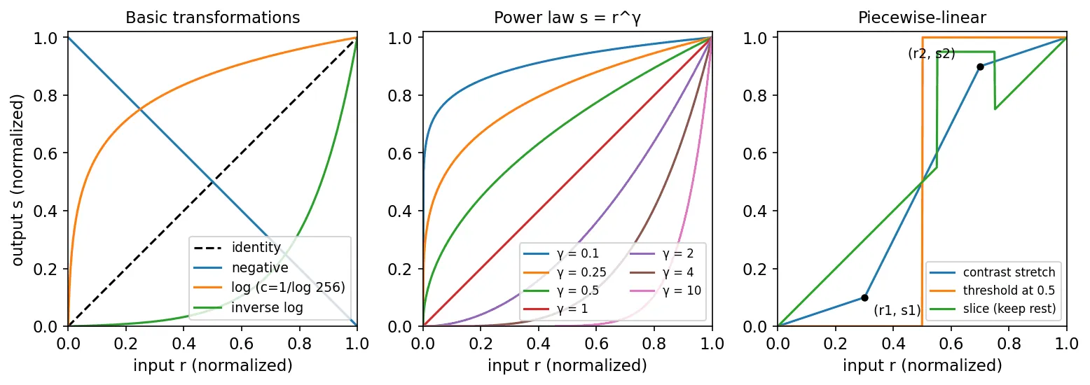
Image negatives

$$s = (L - 1) - r .$$

Dark becomes light and light becomes dark. The slope is $-1$ everywhere, so contrast magnitude is unchanged; only the polarity flips. Negatives help when small bright details sit inside large dark regions, because people often judge gray detail more easily on a light background.

Log transformations

$$s = c \log(1 + r),$$

where $c > 0$ is a scale constant, usually chosen so that the largest input maps to $L - 1$, that is $c = (L-1)/\log L$. The $+1$ keeps $\log 0$ out of the formula. The slope $c/(1 + r)$ is large for small $r$ and small for large $r$. So the log curve expands dark values and compresses bright ones.

Its classic use is displaying data with a huge dynamic range, such as the magnitude of a Fourier spectrum, whose values can span many orders of magnitude. Scaled linearly, only the brightest point is visible. After the log, the structure appears (Figure 3.2, bottom row). The inverse log (exponential) curve does the opposite.

Power-law (gamma) transformations

$$s = c\, r^{\gamma},$$

where $c > 0$ and $\gamma > 0$ are constants (with $r$ normalized to $[0, 1]$, take $c = 1$). For $\gamma < 1$ the curve bows upward and brightens the dark range, like the log. For $\gamma > 1$ it bows downward and darkens it. Unlike the log, one parameter gives a whole family of curves (Figure 3.1, middle).

Gamma matters beyond enhancement. Displays and cameras have power-law responses, and image files usually store gamma-encoded values rather than values proportional to light. Pre-compensating for a device’s response is called gamma correction. One practical consequence: averaging, blurring or resizing gamma-encoded pixels is not the same as doing it on linear light, which is why careful pipelines linearize first.

import numpy as np
from skimage import data, img_as_float

r = img_as_float(data.camera())        # intensities scaled to [0, 1]
negative = 1.0 - r                     # s = (L-1) - r, in normalized form
log_t = np.log1p(r) / np.log(2.0)      # s = c log(1 + r), c chosen so s(1) = 1
bright = r ** 0.4                      # gamma < 1 lifts the shadows
dark = r ** 2.5                        # gamma > 1 deepens them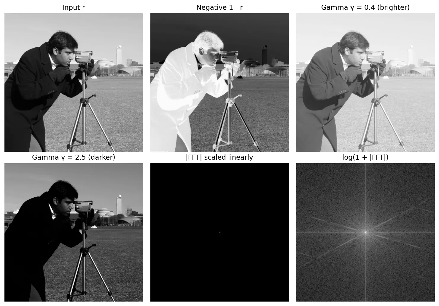

Piecewise-linear transformations

Instead of one formula, we can join straight segments. This gives precise control, at the cost of more parameters.

Contrast stretching. Choose two control points $(r_1, s_1)$ and $(r_2, s_2)$ and connect $(0, 0) \to (r_1, s_1) \to (r_2, s_2) \to (L-1, L-1)$ with straight lines. The middle segment has slope $(s_2 - s_1)/(r_2 - r_1)$. If $r_1 \le r_2$ and $s_1 \le s_2$, the curve is monotonic and never reverses the order of gray levels. Two special cases are worth remembering:

• $r_1 = r_{\min}$, $s_1 = 0$, $r_2 = r_{\max}$, $s_2 = L-1$ maps the image’s actual range onto the full range (a min–max stretch). In practice, use the 1st and 99th percentiles instead of the min and max, so a few outlier pixels do not control the result.
• $r_1 = r_2 = m$, $s_1 = 0$, $s_2 = L - 1$ produces a binary image: a threshold at $m$.

def stretch(img, r1, s1, r2, s2, L=256):
    lut = np.interp(np.arange(L), [0, r1, r2, L - 1], [0, s1, s2, L - 1])
    return lut.astype(np.uint8)[img]

img = data.camera()
lo, hi = np.percentile(img, [1, 99])
out = stretch(img, lo, 0, hi, 255)     # robust min-max stretch

Intensity-level slicing. Highlight one band of intensities $[A, B]$. Either set the band to a high value and everything else to a low value (a binary result), or brighten the band and leave everything else unchanged. Slicing is useful when the gray range of interest is known, such as one tissue type or one material in an X-ray.

Bit-plane slicing. An 8-bit pixel value is a sum of bits, $r = \sum_{b=0}^{7} a_b\, 2^b$ with $a_b \in \{0, 1\}$. Collecting bit $b$ of every pixel gives a binary image called bit plane $b$. Plane 7, the most significant bit (MSB), is exactly a threshold at 128. The low planes look like noise because they carry fine variations. Keeping only the top four planes reconstructs an image that is very close to the original, with a maximum error below $2^4 = 16$ levels (Figure 3.3). This explains why bit planes matter for compression and why the lowest planes are a classic place to hide watermarks.

img = data.camera()                                    # uint8
planes = [(img >> b) & 1 for b in range(8)]            # planes[7] is the MSB
top4 = sum(planes[b].astype(np.uint8) << b for b in range(4, 8))
print(np.abs(img.astype(int) - top4).max())            # 15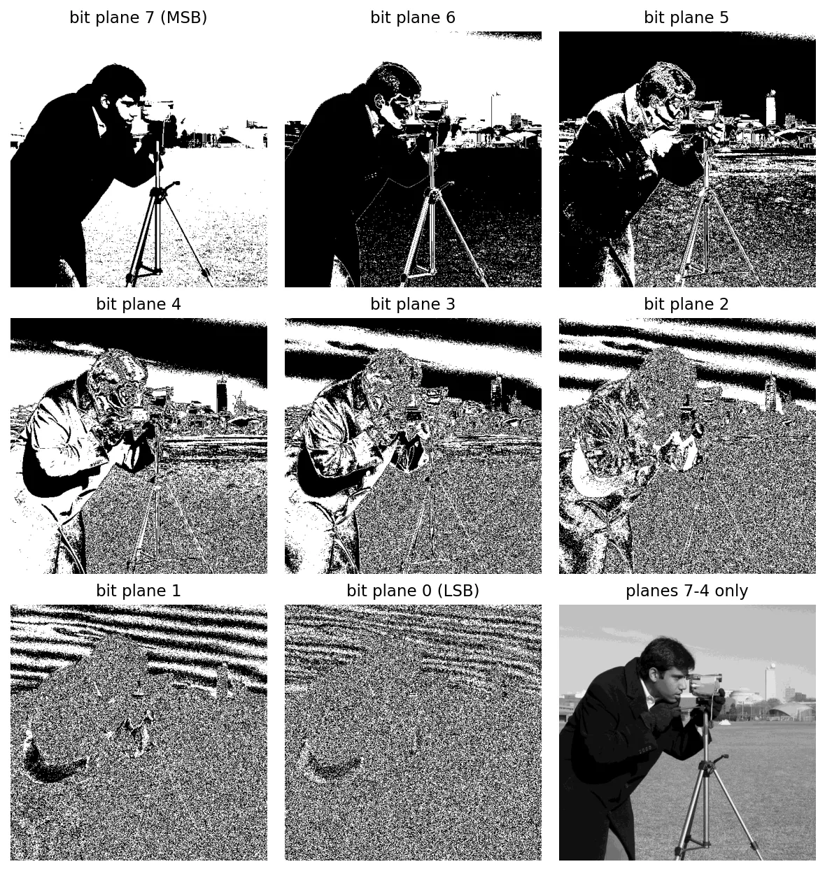

Histogram processing

Plain version. A histogram counts how many pixels have each brightness. A dark image has its counts piled up on the left; a washed-out one has them squeezed into a narrow band. Histogram processing chooses a curve $T$ automatically from those counts, so that the output histogram has a shape we want.

Precise version. For an $M \times N$ image with levels $r_k$, $k = 0, \dots, L-1$, let $n_k$ be the number of pixels with value $r_k$. The normalized histogram

$$p_r(r_k) = \frac{n_k}{MN}$$

is an estimate of the probability that a randomly chosen pixel has value $r_k$. It sums to 1.

Histogram equalization

The goal is a curve $T$ that makes the output histogram as flat as possible, so every gray level is used about equally often.

Derivation (continuous case). Treat intensity as a continuous random variable $r \in [0, L-1]$ with probability density function (PDF) $p_r(r)$. Assume $T$ is strictly increasing on that interval. Then a pixel lands in a small interval $[r, r + dr]$ exactly when its output lands in $[s, s + ds]$ with $s = T(r)$. Equal probabilities give $p_s(s)\,|ds| = p_r(r)\,|dr|$, so

$$p_s(s) = p_r(r) \left| \frac{dr}{ds} \right| .$$

Now choose $T$ as the scaled cumulative distribution function (CDF) of $r$:

$$s = T(r) = (L-1) \int_0^{r} p_r(w)\, dw ,$$

where $w$ is a dummy integration variable. By the fundamental theorem of calculus, $ds/dr = (L-1)\, p_r(r)$. Substituting,

$$p_s(s) = p_r(r) \cdot \frac{1}{(L-1)\, p_r(r)} = \frac{1}{L-1}, \qquad 0 \le s \le L-1 .$$

The output PDF is uniform, whatever the input PDF was. The CDF is the one monotonic curve that spreads probability evenly: it is steep where many pixels live (so they get pulled apart) and flat where few pixels live.

Discrete version. Replace the integral by a sum:

$$s_k = T(r_k) = (L-1) \sum_{j=0}^{k} p_r(r_j), \qquad k = 0, 1, \dots, L-1,$$

and round $s_k$ to the nearest integer. Because many input levels can round to the same output level and no level can be split, the discrete result is only approximately flat. The output histogram usually shows tall spikes separated by gaps (Figure 3.4, middle). What is guaranteed is that the output spans the full range and that the CDF of the output is close to a straight line.

def equalize(img, L=256):
    hist = np.bincount(img.ravel(), minlength=L)      # n_k
    cdf = np.cumsum(hist) / img.size                  # sum of p_r(r_j), j <= k
    lut = np.round((L - 1) * cdf).astype(np.uint8)    # s_k
    return lut[img]

OpenCV’s cv2.equalizeHist uses a slightly different normalization, $(\mathrm{cdf}_k - \mathrm{cdf}_{\min})/(MN - \mathrm{cdf}_{\min})$, so the darkest occupied level maps to 0. Results differ by at most a level or so.

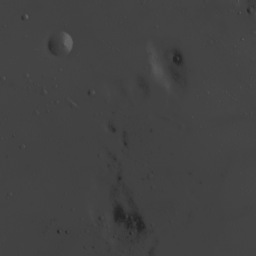
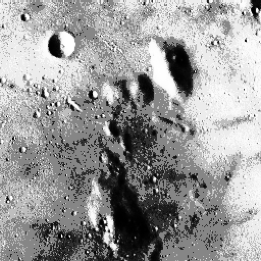
Drag the slider to compare a deliberately low-contrast image with its globally equalized version. Notice that equalization is not “free”: it exaggerates the large smooth areas and grain, because it spends contrast wherever the pixel counts are high, not where the interesting detail is.

InputEqualized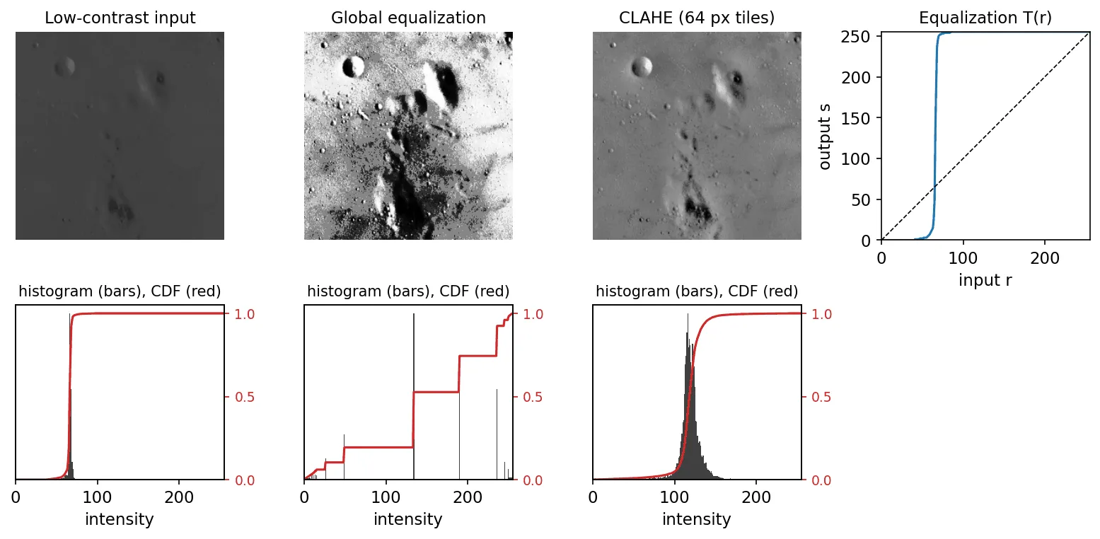

Histogram matching (specification)

Sometimes a flat histogram is the wrong target. We may want an image to look like a reference image, or to have a histogram shape chosen by hand. Histogram matching maps the input so that its histogram approximates a specified PDF $p_z(z)$.

The trick is to use equalization twice. Equalizing the input gives $s = T(r)$ with a uniform $s$. Equalizing the target distribution gives

$$G(z) = (L-1) \int_0^{z} p_z(t)\, dt ,$$

which also yields a uniform variable. Two uniform variables can be matched, so we set $G(z) = T(r)$ and solve:

$$z = G^{-1}\big(T(r)\big).$$

Here $z$ is the output intensity, $G$ is the scaled CDF of the desired distribution and $t$ is a dummy variable. In the discrete case $G$ is a staircase and may not be invertible, so for each input level we take the smallest $z$ with $G(z) \ge T(r)$. That is a single searchsorted call:

def match(img, ref, L=256):
    cdf_in = np.cumsum(np.bincount(img.ravel(), minlength=L)) / img.size
    cdf_ref = np.cumsum(np.bincount(ref.ravel(), minlength=L)) / ref.size
    # For each input level, the smallest z with G(z) >= T(r).
    lut = np.searchsorted(cdf_ref, cdf_in).clip(0, L - 1).astype(np.uint8)
    return lut[img]

skimage.exposure.match_histograms implements the same idea, including per-channel matching for color images.

Exact histogram matching

Both methods above are lookup tables, so all pixels with the same input value receive the same output value. If 30% of the pixels share one value, no lookup table can split them, and the output histogram cannot be exactly flat or exactly match a target.

Exact histogram specification removes this limit by making every pixel distinguishable first [5]. Each pixel gets a vector of features: its own value, then the mean over a small neighborhood, then the mean over a larger one, and so on. Sorting pixels lexicographically by this vector produces a strict ordering in practice, because ties in one feature are broken by the next. Then assign output values in that order: the first $h_0$ pixels get level 0, the next $h_1$ get level 1, and so on, where $h_k$ is the exact count the target histogram requires. The result has precisely the requested histogram. Coltuc, Bolon and Chassery showed that ordering by local means of increasing size gives visually sensible tie-breaking, because pixels in brighter surroundings are pushed slightly upward [5].

Local histogram processing

Global methods use one curve for the whole image. If a dark corner holds the important detail but contains few pixels, the global histogram barely notices it.

Local histogram equalization computes the transformation from the histogram of a neighborhood around each pixel and applies it only to the center pixel, then moves on. Adaptive histogram equalization (AHE) and its variants were studied systematically by Pizer and colleagues, including the problem that AHE over-amplifies noise in nearly uniform regions, where the local histogram is a single spike and the CDF turns into a near-vertical step [2].

Contrast-limited AHE (CLAHE) fixes this by limiting the slope of the mapping. Since the slope of an equalization curve is proportional to the histogram height, clipping each local histogram at a ceiling and redistributing the clipped counts across all bins caps the contrast gain. To make it fast, the image is split into tiles; a mapping is computed per tile, and each pixel’s output is interpolated bilinearly from the four nearest tile mappings, which avoids visible tile seams. Zuiderveld’s Graphics Gems chapter gave the widely reused implementation [3], and Reza described a real-time hardware realization [4].

import cv2
clahe = cv2.createCLAHE(clipLimit=2.0, tileGridSize=(8, 8))
out = clahe.apply(data.moon())         # uint8 in, uint8 out

In scikit-image, the equivalent is skimage.exposure.equalize_adapthist(img, clip_limit=0.01).

Using histogram statistics for image enhancement

A histogram is a distribution, so its moments summarize it. With $p(r_k)$ the normalized histogram, the mean and variance are

$$m = \sum_{k=0}^{L-1} r_k\, p(r_k), \qquad \sigma^2 = \sum_{k=0}^{L-1} (r_k - m)^2\, p(r_k),$$

where $m$ measures average brightness and $\sigma$ (the standard deviation) measures contrast. Computed over a neighborhood $S_{xy}$ centered on $(x, y)$, they become the local mean $m_{S_{xy}}$ and local standard deviation $\sigma_{S_{xy}}$.

These give a simple, targeted enhancement rule. Suppose we want to boost only regions that are dark and have some but not too much contrast (to skip both flat background and strong edges). With global mean $m_G$ and global standard deviation $\sigma_G$, we multiply a pixel by a gain $E > 1$ only if

$$m_{S_{xy}} \le k_0\, m_G \quad \text{and} \quad k_1\, \sigma_G \le \sigma_{S_{xy}} \le k_2\, \sigma_G ,$$

and leave it alone otherwise. Here $k_0, k_1, k_2$ are user-chosen fractions (for example $0.5, 0.02, 0.5$). The local statistics need only two box filters, one on $I$ and one on $I^2$, using $\sigma^2 = \mathbb{E}[I^2] - (\mathbb{E}[I])^2$:

from scipy.ndimage import uniform_filter

f = img_as_float(data.moon())
m = uniform_filter(f, size=3)                                     # local mean
sd = np.sqrt(np.maximum(uniform_filter(f**2, size=3) - m**2, 0))  # local std
mG, sG = f.mean(), f.std()
mask = (m <= 0.5 * mG) & (sd >= 0.02 * sG) & (sd <= 0.5 * sG)
g = np.where(mask, np.clip(3.0 * f, 0, 1), f)                     # gain E = 3

The same “local mean and local variance from box filters” pattern reappears in the guided filter [8], one of the edge-preserving filters discussed in the Modern view.

Fundamentals of spatial filtering

Plain version. A spatial filter slides a small grid of weights (a kernel) across the image. At each position, it multiplies the weights by the pixels underneath and adds the products. The result is the new value of the center pixel.

The convolution tutorial covers the mechanics with a from-scratch NumPy loop, OpenCV calls and border handling. Here we focus on the theory the rest of the chapter needs.

Linear spatial filtering and correlation

Using that tutorial’s notation, for a $(2k+1) \times (2k+1)$ kernel $K$ the correlation of $K$ with $I$ is

$$(K \star I)(x, y) = \sum_{i=-k}^{k} \sum_{j=-k}^{k} K(i, j)\, I(x + i,\; y + j),$$

where $(i, j)$ are offsets from the kernel’s center and $k$ is the kernel’s half-width. Odd sizes give the kernel a well-defined center. The filter is linear because the output is a linear combination of input values: filtering $aI_1 + bI_2$ gives $a$ times the result for $I_1$ plus $b$ times the result for $I_2$. It is also shift-invariant because the same weights are used everywhere.

Correlation versus convolution

Convolution is the same computation with the kernel rotated by 180°:

$$(K * I)(x, y) = \sum_{i=-k}^{k} \sum_{j=-k}^{k} K(i, j)\, I(x - i,\; y - j).$$

The two coincide for kernels that are symmetric under a 180° rotation (box, Gaussian, the Laplacian), and differ for antisymmetric ones (Sobel, any directional derivative), where they produce the same response with opposite sign. The useful difference shows up with an impulse (a single 1 among zeros): correlating a kernel with an impulse produces a rotated copy of the kernel, while convolving produces an exact copy. This is why convolution, not correlation, is the operation with clean algebra:

• commutative: $K * I = I * K$,
• associative: $K_1 * (K_2 * I) = (K_1 * K_2) * I$, so a chain of filters can be merged into one kernel,
• distributive: $K * (I_1 + I_2) = K * I_1 + K * I_2$.

Associativity is what the next two subsections rely on. As noted in the convolution tutorial, cv2.filter2D computes correlation, and most deep-learning “convolution” layers also compute correlation; since their weights are learned, the flip does not matter there.

Separable kernels

A kernel is separable if it is the outer product of a column vector $\mathbf{c}$ and a row vector $\mathbf{r}$:

$$K = \mathbf{c}\, \mathbf{r}^{\top}.$$

Then $K * I = \mathbf{c} * (\mathbf{r}^{\top} * I)$: filter every row with $\mathbf{r}$, then every column with $\mathbf{c}$. For an $m \times n$ kernel this costs $m + n$ multiplications per pixel instead of $mn$, so the speedup is $mn/(m+n)$, which is $3.5\times$ for a $7 \times 7$ kernel and grows linearly with size. A matrix is an outer product exactly when its rank is 1, which also gives a test: compute the singular value decomposition and check that only one singular value is nonzero. Box and Gaussian kernels are separable; so is the Sobel kernel, which is a smoothing vector times a differencing vector.

g1 = cv2.getGaussianKernel(7, 1.5)          # 7x1 column, sums to 1
K = g1 @ g1.T                               # 7x7 Gaussian kernel
print(np.linalg.matrix_rank(K))             # 1  ->  separable
f = img_as_float(data.camera()).astype(np.float32)
a = cv2.filter2D(f, -1, K.astype(np.float32))
b = cv2.sepFilter2D(f, -1, g1, g1)          # two 1-D passes
print(np.abs(a - b).max())                  # ~1e-7

Spatial and frequency domains

The convolution theorem states that convolution in space is multiplication in frequency: if $\mathcal{F}$ denotes the Fourier transform, then $\mathcal{F}\{K * I\} = \mathcal{F}\{K\} \cdot \mathcal{F}\{I\}$. So every linear shift-invariant filter has two equivalent descriptions: a kernel $K$ in space, and a transfer function $H = \mathcal{F}\{K\}$ that says how much of each frequency survives. Smoothing kernels have transfer functions that are large near zero frequency and small at high frequencies: they are lowpass. Sharpening kernels do the opposite: they are highpass. Chapter 4 develops this view properly. For now, the vocabulary is enough: “lowpass” means “smooth”, “highpass” means “edges and detail”.

Small kernels are usually cheaper to apply in space. Very large kernels are often cheaper in frequency via the fast Fourier transform.

Constructing spatial filter kernels

There are three common recipes:

1. From a mathematical property. Averaging gives the box kernel. Derivatives give difference kernels (the Laplacian, Sobel).
2. By sampling a continuous function. Sample a 2-D Gaussian on the integer grid, then normalize the weights to sum to 1.
3. From a frequency specification. Design $H$ in the frequency domain and take its inverse transform to get a spatial kernel, usually truncated to a manageable size.

Two sanity checks apply to all of them. A smoothing kernel’s weights should sum to 1, so flat regions keep their brightness. A derivative kernel’s weights should sum to 0, so flat regions give 0.

Smoothing (lowpass) spatial filters

Plain version. Replace each pixel by an average of its neighborhood. Random noise is pushed toward the average and fades, but sharp edges are also smeared, because the average straddles both sides.

Box filter

The $m \times n$ box kernel has every weight equal to $1/(mn)$. It is the simplest lowpass filter and is separable, and with a running sum it costs a constant amount of work per pixel regardless of size. Its weakness is its frequency response: the transform of a box is a sinc-like function with side lobes, so it lets some high frequencies through with flipped sign, and it smears in a square, direction-dependent way. Small text and thin lines can turn into blocky streaks.

Gaussian filter

The Gaussian kernel samples

$$w(s, t) = C\, e^{-\frac{s^2 + t^2}{2\sigma^2}},$$

where $(s, t)$ are offsets from the kernel’s center, $\sigma$ (the standard deviation) sets the amount of blur, and $C$ is chosen so the weights sum to 1. It has three properties that make it the default smoothing kernel:

• Isotropy. It depends only on the distance $\sqrt{s^2 + t^2}$, so it blurs equally in every direction.
• Separability. $e^{-(s^2+t^2)/2\sigma^2} = e^{-s^2/2\sigma^2}\, e^{-t^2/2\sigma^2}$.
• A smooth, non-negative frequency response. Its Fourier transform is also a Gaussian, so there are no side lobes.

Since about 99.7% of a 1-D Gaussian’s mass is within $\pm 3\sigma$, a kernel of size about $6\sigma$, rounded up to the next odd integer, captures almost all of it. Larger kernels waste work, smaller ones truncate the tails. Convolving two Gaussians with $\sigma_1$ and $\sigma_2$ gives a Gaussian with $\sigma = \sqrt{\sigma_1^2 + \sigma_2^2}$, so repeated small blurs compose predictably.

Order-statistic (nonlinear) filters

Order-statistic filters sort the values in the neighborhood and pick one. They are nonlinear: no kernel can represent them, and the convolution theorem does not apply.

• Median filter: output the middle value (the 50th percentile). It is the standard remedy for impulse noise (salt-and-pepper), isolated pixels forced to black or white. An impulse is an extreme value, so it sorts to the end of the list and is almost never the median. As long as fewer than half the pixels in the window are corrupted, the median ignores them. It also preserves step edges far better than a linear average of the same size.
• Max filter (100th percentile): finds the brightest point; it removes pepper (dark) noise but grows bright specks.
• Min filter (0th percentile): the reverse; removes salt (bright) noise but grows dark specks.

Max and min filters reappear in Chapter 9 as grayscale dilation and erosion.

from scipy import ndimage as ndi

f = img_as_float(data.camera()).astype(np.float32)
noisy = f.copy()
u = np.random.default_rng(0).random(f.shape)
noisy[u < 0.05], noisy[u > 0.95] = 0.0, 1.0       # 10% salt-and-pepper

box = cv2.blur(noisy, (5, 5))
gauss = cv2.GaussianBlur(noisy, (0, 0), sigmaX=1.5)
med = cv2.medianBlur(noisy, 3)
mn, mx = ndi.minimum_filter(noisy, 3), ndi.maximum_filter(noisy, 3)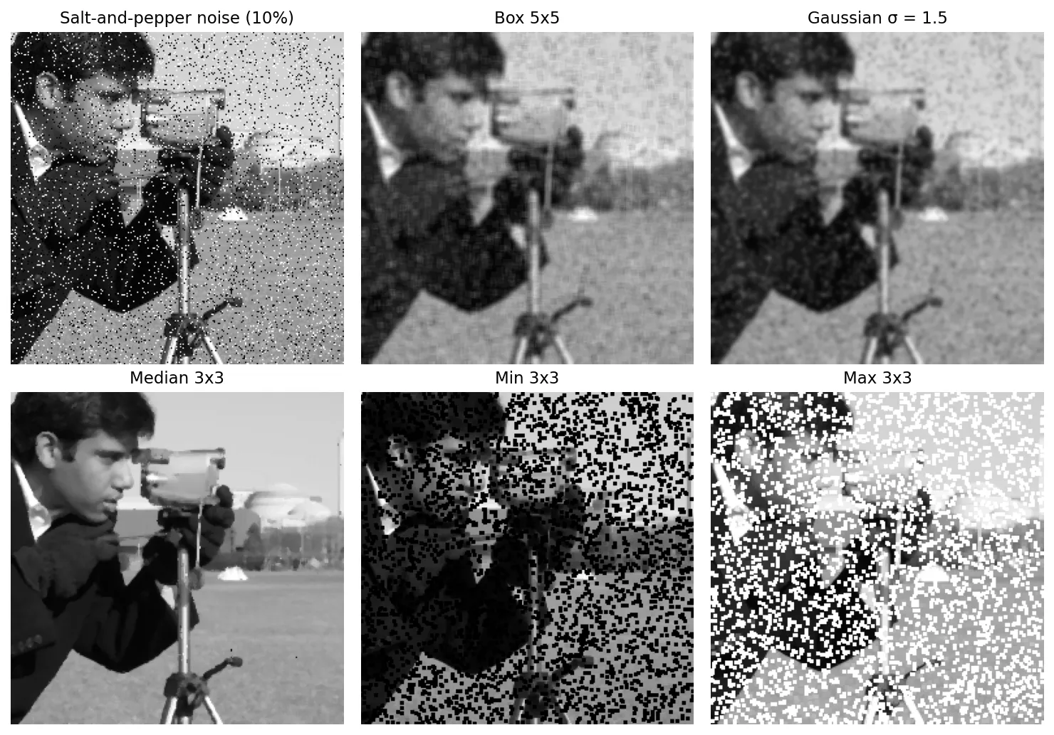

Sharpening (highpass) spatial filters

Plain version. Smoothing averages; sharpening does the opposite and highlights differences. Differences between neighbors are derivatives, so sharpening is built from derivatives.

First and second derivatives

For a 1-D signal $f(x)$ on a pixel grid, the simplest approximations are

$$\frac{\partial f}{\partial x} = f(x+1) - f(x), \qquad \frac{\partial^2 f}{\partial x^2} = f(x+1) + f(x-1) - 2f(x).$$

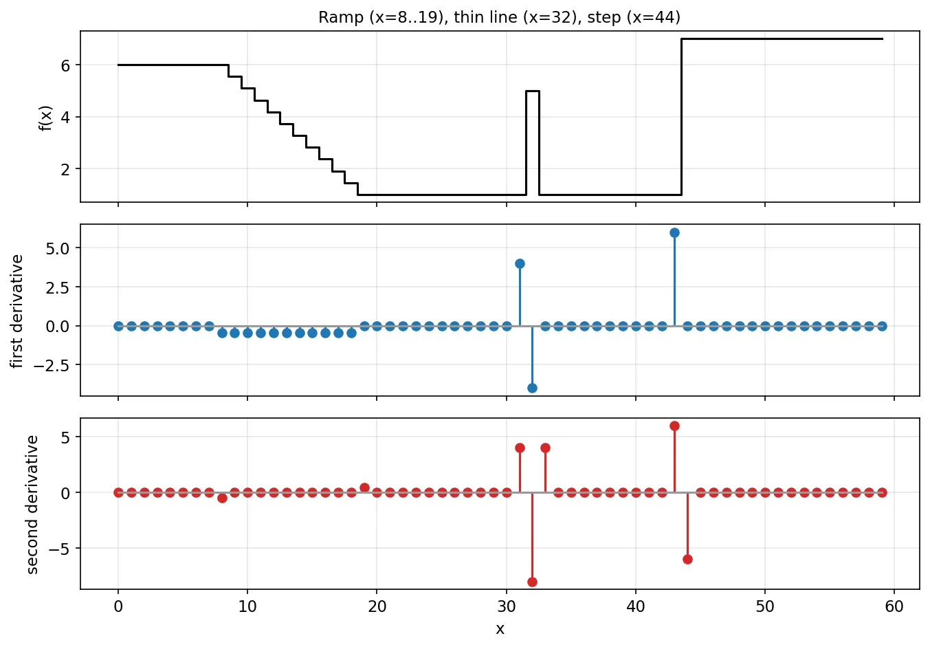
Figure 3.6 applies both to a hand-made profile with a ramp, a one-pixel-wide line and a step. Reading it gives the rules that decide which derivative to use:

• In flat regions, both derivatives are 0.
• Along a ramp, the first derivative is nonzero all the way, which makes thick responses. The second derivative is nonzero only at the ramp’s start and end.
• At a thin line, the second derivative responds strongly with a double response (positive, strong negative, positive), and its magnitude is larger than the first derivative’s. Fine detail is exactly what sharpening should emphasize.
• At a step, the second derivative produces a positive and a negative value next to each other. The zero crossing between them locates the edge precisely, which Chapter 10 uses for edge detection.

So for enhancing fine detail, the second derivative is the more natural choice.

The Laplacian

The simplest isotropic second-derivative operator (one whose response does not change when the image is rotated) is the Laplacian:

$$\nabla^2 I = \frac{\partial^2 I}{\partial x^2} + \frac{\partial^2 I}{\partial y^2}.$$

Adding the 1-D difference above in $x$ and in $y$ gives

$$\nabla^2 I(x, y) = I(x+1, y) + I(x-1, y) + I(x, y+1) + I(x, y-1) - 4I(x, y),$$

which is correlation with the kernel

$$K_{\nabla^2} = \begin{bmatrix} 0 & 1 & 0 \\ 1 & -4 & 1 \\ 0 & 1 & 0 \end{bmatrix}.$$

Adding the two diagonal directions as well gives a version with $1$ in all eight outer cells and $-8$ in the center, which is isotropic in 45° steps instead of 90° steps. Flipping all the signs gives equally valid kernels. The weights sum to 0, so flat regions vanish and only changes survive.

Sharpening with the Laplacian. The Laplacian image is mostly gray (zero) with bright and dark fringes at edges. Adding it back to the original puts those fringes on the edges:

$$G(x, y) = I(x, y) + c\, \nabla^2 I(x, y),$$

where $c = -1$ for kernels with a negative center (like $K_{\nabla^2}$ above) and $c = +1$ for kernels with a positive center. The sign matters: with the wrong sign, edges get blurred instead of sharpened. Because convolution is distributive, $I - \nabla^2 I$ is itself a single kernel, with center $5$ and $-1$ above, below and to each side, which is exactly the sharpen preset in the playground below.

Kernel playgroundEdit any cell or pick a preset. The output updates as you type.

Try the gaussian and box-blur presets for smoothing, then laplacian to see the bare second-derivative response. Changing the center of the sharpen kernel from 5 to 6 makes the weights sum to 2 and brightens the whole image, which shows why the sum matters.

Unsharp masking and highboost filtering

A trick from photographic darkrooms: subtract a blurred copy to isolate the detail, then add the detail back.

$$g_{\text{mask}}(x, y) = I(x, y) - \bar{I}(x, y), \qquad G(x, y) = I(x, y) + \alpha\, g_{\text{mask}}(x, y),$$

where $\bar{I}$ is a blurred (lowpass) version of $I$, $g_{\text{mask}}$ is the unsharp mask (the detail the blur removed), and $\alpha \ge 0$ is a weight. With $\alpha = 1$ this is unsharp masking. With $\alpha > 1$ it is highboost filtering. With $0 \lt \alpha \lt 1$ the effect is gentle. Because $g_{\text{mask}}$ is a highpass signal, this is another way of adding highpass detail, and if $\bar{I}$ is a Gaussian blur, the blur’s $\sigma$ sets the size of the details that get boosted.

Large $\alpha$ causes visible halos: overshoot on both sides of strong edges, and the output may leave the valid range, so clip it.

The gradient and Sobel operators

First derivatives are used through the gradient, the vector of partial derivatives

$$\nabla I = \begin{bmatrix} g_x \\ g_y \end{bmatrix} = \begin{bmatrix} \partial I / \partial x \\ \partial I / \partial y \end{bmatrix},$$

which points in the direction of the fastest increase of intensity. Its length, the gradient magnitude

$$M(x, y) = \sqrt{g_x^2 + g_y^2} \approx |g_x| + |g_y|,$$

is large at edges and near 0 in flat regions. The right-hand approximation avoids the square root but is not isotropic.

The Sobel operators estimate $g_x$ and $g_y$ with $3 \times 3$ kernels:

$$K_x = \begin{bmatrix} -1 & 0 & 1 \\ -2 & 0 & 2 \\ -1 & 0 & 1 \end{bmatrix}, \qquad K_y = \begin{bmatrix} -1 & -2 & -1 \\ 0 & 0 & 0 \\ 1 & 2 & 1 \end{bmatrix}.$$

Each is separable: $K_x = [1, 2, 1]^\top [-1, 0, 1]$, a central difference in one direction multiplied by a small smoothing in the other. The $2$ in the middle gives more weight to the center row or column, which reduces the operator’s sensitivity to noise. (The convolution tutorial uses $K_x$ as its edge-detection example.) The gradient magnitude is rarely used to sharpen directly; it is more often used to find edges, or as a mask that says where sharpening should be allowed, as in the combined example below.

f = img_as_float(data.chelsea()[..., 1]).astype(np.float32)
lap_k = np.array([[0, 1, 0], [1, -4, 1], [0, 1, 0]], np.float32)
lap = cv2.filter2D(f, -1, lap_k)
sharp = np.clip(f - lap, 0, 1)                 # c = -1 because the center is negative

blur = cv2.GaussianBlur(f, (0, 0), 2)
mask = f - blur                                # g_mask
unsharp = np.clip(f + 1.0 * mask, 0, 1)        # alpha = 1
highboost = np.clip(f + 3.0 * mask, 0, 1)      # alpha = 3

gx = cv2.Sobel(f, cv2.CV_32F, 1, 0, ksize=3)
gy = cv2.Sobel(f, cv2.CV_32F, 0, 1, ksize=3)
M = np.hypot(gx, gy)                           # gradient magnitude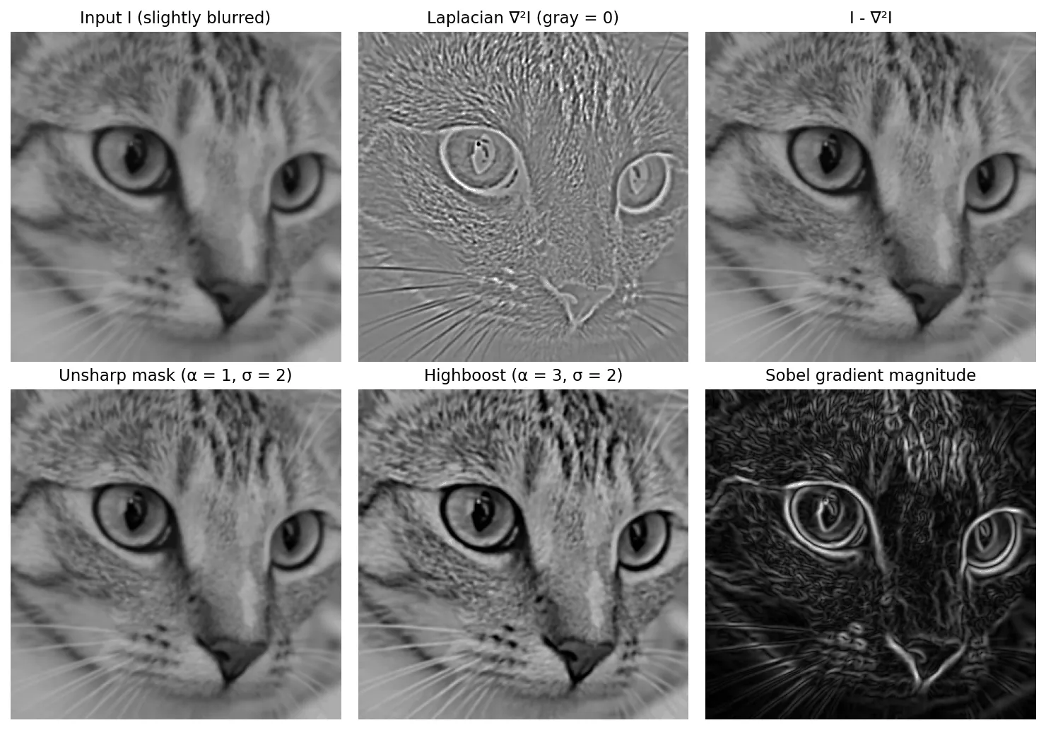

Always filter in floating point. A uint8 pipeline clips the negative values of a Laplacian or a Sobel response to 0 and silently loses half the information.

Highpass, bandreject and bandpass filters from lowpass filters

Plain version. If you know how to keep the smooth part, you also know how to keep everything except the smooth part: subtract.

Let $\delta$ be the unit impulse kernel: a 1 at the center and 0 elsewhere, so $\delta * I = I$. Its transfer function equals 1 at every frequency (an all-pass filter). If $K_{\text{LP}}$ is a lowpass kernel with transfer function $H_{\text{LP}}$, then

$$K_{\text{HP}} = \delta - K_{\text{LP}} \quad\Longleftrightarrow\quad H_{\text{HP}} = 1 - H_{\text{LP}} .$$

Unsharp masking is exactly this: $g_{\text{mask}} = I - \bar{I} = (\delta - K_{\text{LP}}) * I$.

To isolate a band of frequencies, combine two lowpass filters. Let $K_1$ be a Gaussian with small $\sigma_1$ (a high cutoff, so it keeps more detail) and $K_2$ a Gaussian with larger $\sigma_2$ (a low cutoff). Then

$$K_{\text{BP}} = K_1 - K_2, \qquad K_{\text{BR}} = \delta - K_{\text{BP}} = K_2 + (\delta - K_1).$$

The bandpass kernel $K_{\text{BP}}$ keeps frequencies that $K_1$ passes but $K_2$ blocks. The bandreject kernel $K_{\text{BR}}$ is the sum of a lowpass and a highpass and removes only that middle band. The bandpass $K_1 - K_2$ is the difference of Gaussians (DoG), which is also a good approximation of the Laplacian of a Gaussian and is the basis of the scale-space detectors in Chapter 12. The weights confirm the design: highpass and bandpass kernels sum to 0, and the bandreject kernel sums to 1.

def gauss_kernel(sigma):
    n = 2 * int(np.ceil(3 * sigma)) + 1          # about 6 sigma, odd
    g = cv2.getGaussianKernel(n, sigma)
    return g @ g.T

def delta_like(K):
    D = np.zeros_like(K); D[K.shape[0] // 2, K.shape[1] // 2] = 1
    return D

lp2 = gauss_kernel(4.0)                          # low cutoff
lp1 = gauss_kernel(1.0)                          # high cutoff
lp1 = np.pad(lp1, (lp2.shape[0] - lp1.shape[0]) // 2)   # zero-pad to the same size
hp = delta_like(lp1) - lp1                       # highpass, sums to 0
bp = lp1 - lp2                                   # bandpass (DoG), sums to 0
br = delta_like(bp) - bp                         # bandreject, sums to 1

Combining spatial enhancement methods

Plain version. Real images rarely have only one problem. A useful enhancement is usually a short pipeline, and the order of the steps matters.

Here is a worked example. The input (Figure 3.8a) is a portrait that is underexposed, has a little Gaussian noise, and has 4% salt-and-pepper impulses. We want a brighter, crisper picture without amplifying the noise.

1. Remove impulses first, with a 3×3 median filter (b). Impulses are extreme values; any later contrast boost or sharpening would make them worse, and a linear blur would only spread them. The median removes them while keeping edges.
2. Lift the shadows with a gamma of 0.45 (c). A point operation is the right tool for a global brightness problem. Doing it after the median means the curve is not distorted by black and white impulses.
3. Build an edge-weight map (d). Blur the image with a Gaussian ($\sigma = 2$), compute the Sobel gradient magnitude $M$ of the blurred image, and normalize it to $w = \min(M / M_{90}, 1)$, where $M_{90}$ is the 90th percentile of $M$. Because it is computed after smoothing, $w$ is near 1 on real edges and near 0 on the residual noise in flat areas.
4. Apply unsharp masking gated by that map (f): $G = I_c + \alpha\, w \cdot (I_c - \bar{I}_c)$, with $I_c$ the gamma-corrected image, $\bar{I}_c$ its Gaussian blur, $\alpha = 2$, and the product taken pixel by pixel.

Panel (e) shows plain unsharp masking with the same $\alpha$: the background and the dark collar get grainy, because the noise is high-frequency detail too. The gated version (f) sharpens the face, hair and the suit’s outlines nearly as much, while leaving the smooth background clean. This pattern, using a smoothed first-derivative image to decide where a second-order sharpening is applied, is a hand-made version of the edge-aware processing that the Modern view describes.

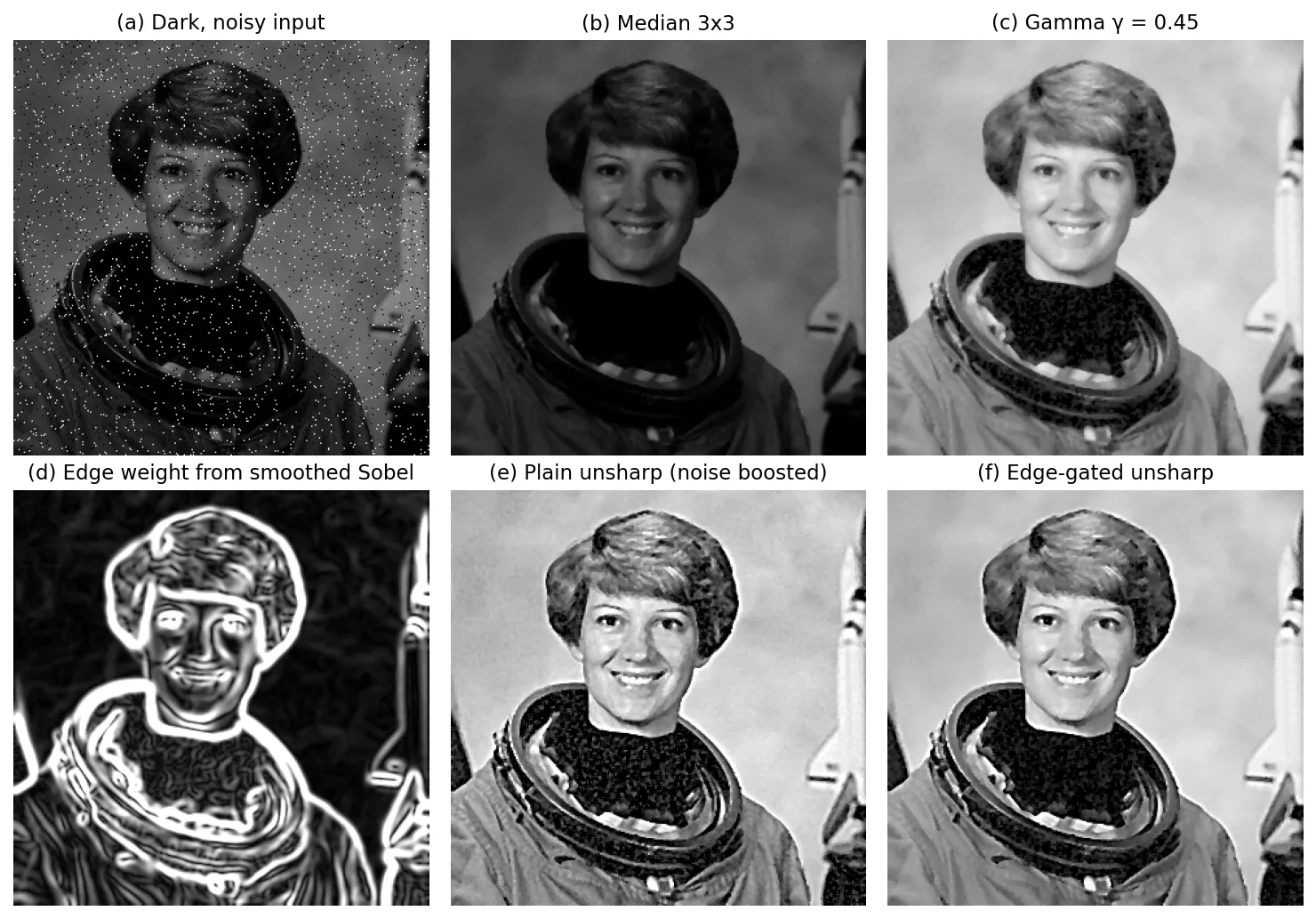
Each step uses one idea from this chapter. The order follows three rules of thumb: remove outliers before any step that amplifies differences, fix global tone with a point operation, and restrict sharpening to where the signal is stronger than the noise.

Modern view

The techniques in this chapter are decades old, and they are still everywhere: CLAHE is a standard preprocessing step in medical imaging and remote sensing, gamma and tone curves are in every camera pipeline, and Gaussian, median and Sobel filters are in every vision library. Research since has pushed in three directions: smarter contrast enhancement, filters that smooth without blurring edges, and learned replacements for both. The surveys below are good entry points.

Contrast enhancement and histogram methods. Pizer et al. [2] remains the reference analysis of adaptive histogram equalization: it describes how local mappings behave, why AHE over-enhances noise in uniform regions, and the variants (including contrast limiting and interpolation between tile mappings) that made the method practical. Zuiderveld’s chapter [3] is the compact CLAHE implementation that later libraries follow, and Reza [4] shows the same algorithm mapped to real-time hardware. On the histogram-specification side, Coltuc, Bolon and Chassery [5] show how to obtain an exact target histogram by strictly ordering pixels with local means. For a broader map of the field, Qi et al. [11] survey image-enhancement methods from the past two decades, organizing them into supervised and unsupervised algorithms and covering quality evaluation as a third pillar; it is useful for its side-by-side discussion of the limitations, merits and drawbacks of each family.

Edge-preserving filters. The weakness of the box and Gaussian filters is that they average across edges. The bilateral filter of Tomasi and Manduchi [6] fixes this by multiplying the spatial Gaussian weight by a second weight that decays with intensity difference, so a pixel on the other side of an edge contributes little. The survey by Paris, Kornprobst, Tumblin and Durand [7] explains its behavior, fast implementations and applications such as tone mapping and detail enhancement, where an image is split into a smooth base layer and a detail layer. The guided filter of He, Sun and Tang [8] assumes that the output is a local linear function of a guidance image. It is computed only with box filters of local means and variances, so its cost does not depend on the radius, and it behaves better than the bilateral filter near strong edges, where the bilateral filter can produce gradient-reversal artifacts in detail enhancement. Milanfar’s tutorial [9] unifies bilateral, non-local means and related filters as data-adaptive weighted averages, where the kernel weights depend on the image itself, and analyzes them with linear-algebra tools. Gingichashvili and Lischinski [10] point out that the many edge-preserving filters had been compared mostly by eye, and propose a systematic methodology and common baseline for evaluating them.

How deep learning changed things. The most interesting finding is how much of this chapter survives inside learned systems. Many successful enhancement networks do not output pixels directly; they predict the parameters of a classical operator and then apply it.

• Learned curves. Zero-DCE [13] (2020) predicts pixel-wise, high-order curves (built by iterating a simple quadratic of the form $s = r + a\, r(1 - r)$, with $a$ predicted per pixel) to brighten low-light images. It is trained without any reference images, using non-reference losses that score the enhanced result directly. It is the gamma and contrast-stretching idea, with the curve chosen per pixel by a small CNN.
• Learned lookup tables. Zeng et al. [14] (2020) learn a few basis 3-D color lookup tables and a tiny CNN that predicts how to blend them for each image, which runs in real time on high-resolution photos. This is the lookup-table view of intensity transformations, extended from gray levels to color.
• Learned edge-aware filters. HDRNet by Gharbi et al. [15] predicts local affine color transforms in a low-resolution bilateral grid and applies them at full resolution guided by the input, which is the bilateral filter’s edge-awareness turned into a learned layer. Wu et al. [16] made the guided filter a differentiable layer that can be trained end-to-end inside a network.
• Low-light enhancement. The survey by Li et al. [12] reviews deep low-light image and video enhancement by learning strategy, network structure, loss functions and training data, and introduces a new low-light dataset captured with various phones under diverse illumination, plus an online platform for comparing methods. Later models such as Retinexformer [17] (2023) combine the Retinex model (an image as illumination times reflectance) with transformer attention guided by an illumination estimate.

What did not change: the median filter is still the first answer to impulse noise, the Sobel kernels still appear in loss functions and edge maps, CLAHE is still a default preprocessing step, and gamma handling remains a source of bugs in learned pipelines that mix linear and encoded pixel values. Deep models also tend to inherit the classical failure modes: halos, noise amplification in dark regions and over-enhancement are still the artifacts that reviewers look for.

Key takeaways

• An intensity transformation $s = T(r)$ is a lookup table; its slope is the local contrast gain. Log and $\gamma \lt 1$ curves expand the shadows, $\gamma > 1$ expands the highlights, and piecewise-linear curves give precise control.
• Histogram equalization uses the scaled CDF as $T$, which makes the output PDF uniform in the continuous case and approximately flat in the discrete case. Matching chains one equalization with the inverse of another; exact matching first breaks ties with local means.
• Local methods (AHE, CLAHE, local mean and variance rules) adapt to regions; CLAHE limits the contrast gain by clipping each local histogram.
• Linear spatial filtering is correlation with a kernel; convolution flips the kernel and has clean algebra. Separable kernels cost $m + n$ instead of $mn$ operations per pixel.
• Lowpass filters (box, Gaussian) average away noise and blur edges; the nonlinear median filter is the tool for impulse noise.
• Sharpening adds highpass detail: the Laplacian (second derivative), unsharp masking and highboost, while the gradient and Sobel operators measure edge strength.
• Highpass, bandpass and bandreject kernels follow from lowpass ones by subtraction from the impulse $\delta$; good pipelines order steps so that nothing amplifies what an earlier step should have removed.

Exercises

1. A curve for a foggy photo. An 8-bit image has all its pixels between 90 and 160. Write the piecewise-linear transformation that maps this range onto $[0, 255]$, give its slope, and say what happens to two neighboring pixels with values 120 and 122.

Hint

$T(r) = 255\,(r - 90)/70$ for $90 \le r \le 160$, clipped to $[0, 255]$ outside. The slope is $255/70 \approx 3.64$, so a difference of 2 becomes about 7.3 gray levels. After rounding, $T(120) = 109$ and $T(122) = 117$.

2. Equalize by hand. A tiny 3-bit image ($L = 8$) with 16 pixels has counts $n = [0, 8, 4, 2, 2, 0, 0, 0]$ for levels $0$ to $7$. Compute the equalization lookup table and the output histogram. Why is the output not flat?

Hint

The CDF is $[0, 0.5, 0.75, 0.875, 1, 1, 1, 1]$, so $s_k = \mathrm{round}(7 \cdot \mathrm{CDF})$ gives $[0, 4, 5, 6, 7, 7, 7, 7]$ (with $3.5$ rounded to 4). The output histogram has 8 pixels at level 4, 4 at 5, 2 at 6 and 2 at 7. The 8 pixels at level 1 share one input value, and a lookup table cannot split them. Only exact histogram specification could.

3. Does order matter? Is applying a gamma curve and then a box (averaging) filter the same as applying the box filter and then the gamma curve? Prove your answer or give a counterexample using a 2-pixel average.

Hint

No. Take a 1-D average of two pixels, 0 and 1, with $\gamma = 2$. Gamma first: $(0 + 1)/2 = 0.5$. Box first: $0.5^2 = 0.25$. A nonlinear point operation does not commute with a linear filter. This is also why blurring gamma-encoded images is not the same as blurring linear light.

4. Separable or not? Decide whether each kernel is separable, and if so, give the two vectors: (a) the $3 \times 3$ Laplacian with $-4$ in the center; (b) the $3 \times 3$ kernel with all entries 1; (c) $\begin{bmatrix} 1 & 2 & 1 \\ 2 & 4 & 2 \\ 1 & 2 & 1 \end{bmatrix}$.

Hint

(a) No: its rank is 2 (but it is the sum of two separable kernels, one per axis). (b) Yes: $[1,1,1]^\top[1,1,1]$. (c) Yes: $[1,2,1]^\top[1,2,1]$, a small binomial approximation of a Gaussian. Check with np.linalg.matrix_rank.

5. Median versus mean on an edge. A 1-D signal is $[10, 10, 10, 10, 50, 50, 50, 50]$, a perfect step. Apply a 3-sample mean and a 3-sample median (ignore the end samples). Then replace the sample at position 1 (counting from 0) with an impulse of value 255 and repeat. What do you conclude?

Hint

On the clean step, the mean gives a ramp ($\dots, 10, 23.3, 36.7, 50, \dots$) while the median keeps the step exactly. With the impulse, the mean turns it into two raised values of about 92 at positions 1 and 2; the median outputs 10 there and removes it completely.

6. Design a bandpass kernel. Using Gaussians with $\sigma_1 = 1$ and $\sigma_2 = 3$, build a bandpass kernel and a bandreject kernel in NumPy. Verify the sums of their weights, filter skimage.data.brick() with both, and describe which structures each output keeps.

Hint

Make both kernels the same size (pad the smaller one with zeros), then use $K_1 - K_2$ and $\delta - (K_1 - K_2)$. Sums should be about 0 and 1. The bandpass output keeps the mortar lines and the brick-scale texture, removing both the overall shading and the finest grain; the bandreject output keeps shading and fine grain but weakens the brick pattern.

References

1. R. C. Gonzalez and R. E. Woods, Digital Image Processing, 4th ed., Pearson, 2018, Ch. 3. publisher page
2. S. M. Pizer, E. P. Amburn, J. D. Austin, R. Cromartie, A. Geselowitz, T. Greer, B. ter Haar Romeny, J. B. Zimmerman and K. Zuiderveld, “Adaptive histogram equalization and its variations,” Computer Vision, Graphics, and Image Processing, 1987. doi
3. K. Zuiderveld, “Contrast limited adaptive histogram equalization,” in P. S. Heckbert (ed.), Graphics Gems IV, Morgan Kaufmann, 1994, pp. 474–485. entry
4. A. M. Reza, “Realization of the contrast limited adaptive histogram equalization (CLAHE) for real-time image enhancement,” Journal of VLSI Signal Processing, 2004. doi
5. D. Coltuc, P. Bolon and J.-M. Chassery, “Exact histogram specification,” IEEE Transactions on Image Processing, 2006. doi
6. C. Tomasi and R. Manduchi, “Bilateral filtering for gray and color images,” in Proc. IEEE International Conference on Computer Vision (ICCV), 1998. pdf
7. S. Paris, P. Kornprobst, J. Tumblin and F. Durand, “Bilateral filtering: Theory and applications,” Foundations and Trends in Computer Graphics and Vision, vol. 4, no. 1, pp. 1–73, 2009. doi
8. K. He, J. Sun and X. Tang, “Guided image filtering,” in Proc. European Conference on Computer Vision (ECCV), 2010, pp. 1–14; extended version in IEEE TPAMI, 2013. doi
9. P. Milanfar, “A tour of modern image filtering,” IEEE Signal Processing Magazine, vol. 30, no. 1, pp. 106–128, 2013. IEEE Xplore
10. S. Gingichashvili and D. Lischinski, “Evaluation and comparison of edge-preserving filters,” arXiv:2012.13778, 2020. arXiv
11. Y. Qi, Z. Yang, W. Sun et al., “A comprehensive overview of image enhancement techniques,” Archives of Computational Methods in Engineering, 2021. doi
12. C. Li, C. Guo, L. Han, J. Jiang, M.-M. Cheng, J. Gu and C. C. Loy, “Low-light image and video enhancement using deep learning: A survey,” IEEE Transactions on Pattern Analysis and Machine Intelligence, 2021 (arXiv:2104.10729). arXiv
13. C. Guo, C. Li, J. Guo, C. C. Loy, J. Hou, S. Kwong and R. Cong, “Zero-reference deep curve estimation for low-light image enhancement,” in Proc. IEEE/CVF CVPR, 2020. arXiv
14. H. Zeng, J. Cai, L. Li, Z. Cao and L. Zhang, “Learning image-adaptive 3D lookup tables for high performance photo enhancement in real-time,” IEEE Transactions on Pattern Analysis and Machine Intelligence, 2020. arXiv
15. M. Gharbi, J. Chen, J. T. Barron, S. W. Hasinoff and F. Durand, “Deep bilateral learning for real-time image enhancement,” ACM Transactions on Graphics (SIGGRAPH), 2017. arXiv
16. H. Wu, S. Zheng, J. Zhang and K. Huang, “Fast end-to-end trainable guided filter,” in Proc. IEEE/CVF CVPR, 2018. arXiv
17. Y. Cai, H. Bian, J. Lin, H. Wang, R. Timofte and Y. Zhang, “Retinexformer: One-stage Retinex-based transformer for low-light image enhancement,” in Proc. IEEE/CVF ICCV, 2023. arXiv