Chapter 6 · Color Image Processing

What you’ll learn

• Why three numbers are enough to describe a color for a human observer, and what the CIE chromaticity diagram and a device gamut are
• How the RGB, CMY(K), HSI and CIE L*a*b* models relate, with exact conversion formulas, plus where sRGB gamma and YCbCr fit in
• How pseudocolor turns a grayscale image into a readable color picture, and why perceptually uniform colormaps such as viridis beat the rainbow
• How to transform, white-balance, equalize, smooth, sharpen and segment full-color images, and when to process channels separately versus as vectors
• How noise behaves in color images and how vector filters remove it
• What modern research (learning-based color constancy, colormap design, deep colorization) adds to the classical toolkit

The big picture

So far every pixel has been one number: its brightness. Color images store three numbers per pixel. Color helps us find objects (“the red car”) and separate materials, and it is the first thing people notice when a photo looks wrong.

Following the textbook [1], the chapter answers three questions: how to describe color precisely (fundamentals and models), how to use color to show data that is not colorful (pseudocolor), and how to process real color photographs (transformations, filtering, segmentation, noise, compression). Most grayscale tools from Chapters 3 to 5 carry over, with one recurring twist: a color pixel is a vector, and treating it as three unrelated numbers is sometimes fine and sometimes badly wrong.

Color fundamentals

In plain words. Light is a mix of wavelengths. Our eyes do not measure that whole mix. They squash it into three numbers, one per type of color sensor. Two very different light mixes that produce the same three numbers look identical to us.

Light, cones and trichromacy

Visible light spans wavelengths of roughly 400 to 700 nanometers. A light source or a surface is described by its spectral power distribution $S(\lambda)$: how much energy it emits or reflects at each wavelength $\lambda$.

The retina has three kinds of cones (color-sensitive photoreceptors), most sensitive to short, medium and long wavelengths. Each cone type $c \in \{S, M, L\}$ has a sensitivity curve $s_c(\lambda)$, and its response is

$$r_c = \int S(\lambda)\, s_c(\lambda)\, d\lambda .$$

Here $S(\lambda)$ is the incoming spectrum and $s_c(\lambda)$ the sensitivity of cone type $c$. Because a whole spectrum is reduced to three numbers, human color vision is trichromatic. A direct consequence is metamerism: two different spectra $S_1 \neq S_2$ that give the same three responses look like the same color. Metamerism is why displays work: a monitor never reproduces a lemon’s spectrum, only its three cone responses.

Brightness, hue and saturation

People describe a color with three perceptual attributes:

• Brightness: how much light seems to be there (for a colorless gray, this is all there is).
• Hue: the dominant wavelength, the thing we name with words such as red, orange or blue.
• Saturation: how pure the color is, i.e. how little white is mixed in. Pink is a low-saturation red.

Hue and saturation together are called chromaticity, so a color is “chromaticity plus brightness”, the idea behind the HSI model.

CIE tristimulus values and the chromaticity diagram

To make color measurable, the Commission Internationale de l’Éclairage (CIE) standardized, in 1931, three color-matching functions $\bar{x}(\lambda), \bar{y}(\lambda), \bar{z}(\lambda)$ derived from human matching experiments. The tristimulus values of a spectrum are

$$X = \int S(\lambda)\,\bar{x}(\lambda)\,d\lambda, \qquad Y = \int S(\lambda)\,\bar{y}(\lambda)\,d\lambda, \qquad Z = \int S(\lambda)\,\bar{z}(\lambda)\,d\lambda .$$

$X, Y, Z$ are non-negative by construction, and $\bar{y}$ was chosen to match the eye’s brightness sensitivity, so $Y$ is the luminance. To separate chromaticity from brightness, normalize:

$$x = \frac{X}{X+Y+Z}, \qquad y = \frac{Y}{X+Y+Z}, \qquad z = \frac{Z}{X+Y+Z} = 1 - x - y .$$

$x, y$ are the chromaticity coordinates; $z$ is redundant. Plotting every pure spectral color (a single wavelength) in the $(x, y)$ plane traces a horseshoe-shaped curve called the spectral locus. The straight line joining its two ends is the line of purples (purples are not single wavelengths). Every color a human can see lies inside this region.

Two geometric facts make the diagram useful:

1. Mixing is linear. Any mixture of two lights lies on the straight segment between their chromaticities. Any mixture of three lights lies inside their triangle.
2. White sits in the middle. A reference white, for example the daylight illuminant D65 at $(x, y) \approx (0.3127, 0.3290)$, lies near the center. Moving from white toward the locus increases saturation; the direction gives the hue.

Gamut

A display with three primaries can only produce the colors inside the triangle formed by those primaries. That triangle is the device’s gamut. Because the spectral locus is curved, no triangle with physically realizable corners can cover it. Every three-primary display therefore misses some visible colors, especially saturated cyans and greens.

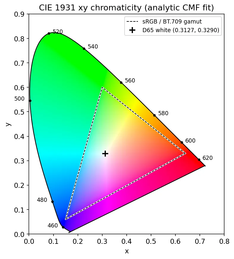
The tabulated CIE functions are long tables; Wyman, Sloan and Shirley [2] give a fit made of a few piecewise Gaussians that is accurate enough for figures like this one. Each lobe is $a\,\exp\!\big(-\tfrac12 t^2\big)$ with $t = (\lambda-\mu)/\sigma$, where the width $\sigma$ differs on the left and right of the peak $\mu$.

Color models

In plain words. A color model is a coordinate system for colors. Different jobs need different coordinates: screens think in red-green-blue light, printers in inks, and people in “which color, how vivid, how bright”.

RGB

In the RGB model each color is a point $(R, G, B)$ in a unit cube. Black is $(0,0,0)$, white is $(1,1,1)$, and the main diagonal holds the grays. An 8-bit-per-channel image has $2^{24} \approx 16.7$ million possible colors. RGB is additive: it describes light being added together, which is how displays and camera sensors work.

“RGB” alone is not a precise color: $(1, 0, 0)$ means a different red on every display. The sRGB standard [3] fixes this by specifying primaries (the same chromaticities as ITU-R BT.709 [4]), the D65 white point, and a nonlinear encoding. The encoding, often loosely called “gamma”, converts a stored value $C' \in [0,1]$ to linear light $C$:

$$C = \begin{cases} C'/12.92, & C' \le 0.04045,\\[2pt] \left(\dfrac{C' + 0.055}{1.055}\right)^{2.4}, & C' > 0.04045. \end{cases}$$

$C'$ is the stored (encoded) value of one channel and $C$ the linear-light value. The curve spends more code values on dark tones, where the eye is more sensitive. Practical rule: operations that model physics (blurring, resizing, mixing light) are more correct on linear values, so decode first when accuracy matters.

CMY and CMYK

Printing works the other way round. Ink on white paper removes light, so printing is subtractive. The secondary colors cyan, magenta and yellow absorb red, green and blue respectively. With values in $[0,1]$:

$$\begin{bmatrix} C \\ M \\ Y \end{bmatrix} = \begin{bmatrix} 1 \\ 1 \\ 1 \end{bmatrix} - \begin{bmatrix} R \\ G \\ B \end{bmatrix} .$$

Here $C, M, Y$ are ink amounts (not to be confused with the CIE $Y$). Equal amounts of real C, M and Y inks give a muddy brown, not black, so printers add a fourth black ink $K$. A simple conversion is

$$K = \min(C, M, Y), \qquad C_K = \frac{C - K}{1 - K}, \quad M_K = \frac{M - K}{1 - K}, \quad Y_K = \frac{Y - K}{1 - K} \quad (K < 1),$$

with $C_K = M_K = Y_K = 0$ when $K = 1$ (pure black). Real printers use measured profiles instead, but the idea is the same: move the shared gray part into black ink.

HSI

RGB is convenient for hardware but awkward for people: nobody describes a color as “70% red, 40% green, 20% blue”. The HSI model (hue, saturation, intensity) decouples brightness from chromaticity, which matches how we talk about color and makes many algorithms simpler.

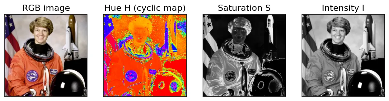
Geometrically, stand the RGB cube on its black corner so the gray diagonal points up. Intensity is the height along that axis. Cut the cube with a plane perpendicular to the axis: hue is the angle around the axis (red at $0^\circ$, green at $120^\circ$, blue at $240^\circ$), and saturation is the distance from the axis.

RGB to HSI (with $R, G, B \in [0, 1]$):

$$\theta = \cos^{-1}\!\left( \frac{\tfrac12\big[(R-G)+(R-B)\big]}{\sqrt{(R-G)^2 + (R-B)(G-B)}} \right), \qquad H = \begin{cases} \theta, & B \le G \\ 360^\circ - \theta, & B > G \end{cases}$$ $$S = 1 - \frac{3\,\min(R, G, B)}{R + G + B}, \qquad I = \frac{R + G + B}{3} .$$

$\theta$ is the angle between the pixel’s chromatic component and the red axis. $H$ is hue in degrees, $S \in [0,1]$ saturation, $I \in [0,1]$ intensity. Two edge cases need care in code. For gray pixels ($R = G = B$) the denominator of $\theta$ is zero and hue is undefined; set it to $0$ by convention. For black ($I = 0$) saturation is undefined; set it to $0$ as well.

HSI to RGB depends on which $120^\circ$ sector $H$ falls in. In the RG sector ($0^\circ \le H < 120^\circ$):

$$B = I(1 - S), \qquad R = I\left[1 + \frac{S \cos H}{\cos(60^\circ - H)}\right], \qquad G = 3I - (R + B).$$

In the GB sector ($120^\circ \le H < 240^\circ$) subtract $120^\circ$ from $H$ and apply the same three formulas with $(B, R, G)$ replaced by $(R, G, B)$. In the BR sector ($240^\circ \le H < 360^\circ$) subtract $240^\circ$ and replace $(B, R, G)$ by $(G, B, R)$. In each sector the channel “opposite” the hue gets the smallest value $I(1-S)$.

import numpy as np

def rgb_to_hsi(rgb):
    """rgb: float array in [0, 1] with shape (..., 3). Returns H (degrees), S, I."""
    R, G, B = rgb[..., 0], rgb[..., 1], rgb[..., 2]
    num = 0.5 * ((R - G) + (R - B))
    den = np.sqrt((R - G) ** 2 + (R - B) * (G - B))
    theta = np.degrees(np.arccos(np.clip(num / (den + 1e-12), -1, 1)))
    H = np.where(B > G, 360.0 - theta, theta)
    I = rgb.mean(axis=-1)
    S = np.where(I > 0, 1 - rgb.min(axis=-1) / (I + 1e-12), 0.0)
    H = np.where(den > 1e-12, H, 0.0)      # gray pixels: hue undefined -> 0
    return H, S, I

def hsi_to_rgb(H, S, I):
    """H in degrees, S and I in [0, 1]. Inverse of rgb_to_hsi."""
    H = np.mod(H, 360.0)
    out = np.zeros(H.shape + (3,))
    # (sector start, index of the 'big' channel, of the smallest, of the rest)
    for lo, (a, b, c) in ((0, (0, 2, 1)), (120, (1, 0, 2)), (240, (2, 1, 0))):
        m = (H >= lo) & (H < lo + 120)
        h = np.radians(H[m] - lo)
        x = I[m] * (1 - S[m])
        y = I[m] * (1 + S[m] * np.cos(h) / np.cos(np.radians(60) - h))
        out[m, a], out[m, b], out[m, c] = y, x, 3 * I[m] - (x + y)
    return out

prim = np.array([[1, 0, 0], [0, 1, 0], [0, 0, 1], [0.5, 0.5, 0.5]], float)
print(np.round(np.stack(rgb_to_hsi(prim), -1), 3))
# [[  0.   1.   0.333] [120.  1.  0.333] [240.  1.  0.333] [  0.  0.  0.5 ]]

The round trip hsi_to_rgb(*rgb_to_hsi(x)) reproduces random RGB inputs to within about $10^{-9}$.

CIE L*a*b*

HSI separates brightness from chromaticity, but equal steps in HSI do not look equally large. The CIE 1976 L*a*b* space [5] was designed so that Euclidean distance roughly tracks perceived difference. It is computed from tristimulus values relative to a reference white $(X_n, Y_n, Z_n)$:

$$L^* = 116\, f\!\left(\frac{Y}{Y_n}\right) - 16, \qquad a^* = 500\left[f\!\left(\frac{X}{X_n}\right) - f\!\left(\frac{Y}{Y_n}\right)\right], \qquad b^* = 200\left[f\!\left(\frac{Y}{Y_n}\right) - f\!\left(\frac{Z}{Z_n}\right)\right],$$ $$f(t) = \begin{cases} t^{1/3}, & t > \delta^3 \\ \dfrac{t}{3\delta^2} + \dfrac{4}{29}, & t \le \delta^3 \end{cases} \qquad \delta = \frac{6}{29}.$$

$L^* \in [0, 100]$ is lightness, $a^*$ runs from green (negative) to red (positive), and $b^*$ from blue (negative) to yellow (positive). The cube root mimics the eye’s compressive response, and the linear piece avoids an infinite slope near black. The color difference $\Delta E^*_{ab}$ is the Euclidean distance between two $(L^*, a^*, b^*)$ points.

To get there from an sRGB file: decode the gamma (formula above), multiply the linear RGB by the sRGB-to-XYZ matrix, then apply the formulas with the D65 white.

import numpy as np
from skimage import color

M = np.array([[0.4124, 0.3576, 0.1805],      # linear sRGB -> XYZ (D65)
              [0.2126, 0.7152, 0.0722],
              [0.0193, 0.1192, 0.9505]])

def srgb_to_lab(rgb):
    lin = np.where(rgb <= 0.04045, rgb / 12.92, ((rgb + 0.055) / 1.055) ** 2.4)
    xyz = lin @ M.T / np.array([0.95047, 1.0, 1.08883])   # divide by D65 white
    d = 6 / 29
    f = np.where(xyz > d**3, np.cbrt(xyz), xyz / (3 * d**2) + 4 / 29)
    return np.stack([116 * f[..., 1] - 16,
                     500 * (f[..., 0] - f[..., 1]),
                     200 * (f[..., 1] - f[..., 2])], -1)

x = np.random.default_rng(0).random((1000, 3))
print(np.abs(srgb_to_lab(x) - color.rgb2lab(x[None])[0]).max())   # about 0.02

The small residual comes from rounding in the matrix; skimage.color.rgb2lab uses more digits.

YCbCr in one paragraph

Video and image codecs separate a luma signal $Y'$ from two chroma differences, because the eye resolves fine detail in brightness much better than in color. ITU-R BT.601 [6] defines, for gamma-encoded $R', G', B' \in [0,1]$,

$$Y' = 0.299\,R' + 0.587\,G' + 0.114\,B',$$

with $C_b \propto B' - Y'$ and $C_r \propto R' - Y'$ scaled and offset into 8-bit “studio” ranges ($Y'$ in $[16, 235]$, $C_b, C_r$ in $[16, 240]$). HDTV uses BT.709 [4], whose luma weights are different ($0.2126, 0.7152, 0.0722$). Mixing them up shifts colors slightly but visibly. skimage.color.rgb2ycbcr implements the BT.601 studio-range version.

Pseudocolor image processing

In plain words. Pseudocolor (false color) paints a grayscale image with colors so that small differences in brightness become easy to see. The colors are not “real”; they are a code, like the colors on a weather map.

The motivation is perceptual: people can tell apart far more color combinations than shades of gray. A thermal camera, an X-ray, a depth map or an elevation model only has one value per pixel, but rendering that value with color can reveal structure the eye would miss in gray.

Intensity slicing

The simplest scheme cuts the gray range into bands and gives each band a color. With thresholds $0 = l_0 < l_1 < \dots < l_P = L-1$ and colors $c_1, \dots, c_P$,

$$g(x, y) = c_k \quad \text{if} \quad l_{k-1} \le f(x, y) < l_k .$$

$f$ is the input gray level, $L$ the number of gray levels, $P$ the number of bands, and $g$ the output color. Viewed as a 3-D plot of $f$, each threshold is a horizontal plane slicing the “intensity terrain”, hence the name. With $P = 2$ this is plain thresholding drawn in two colors. Intensity slicing is ideal when the bands mean something: “temperature above 40 °C”, “bone versus soft tissue”.

Intensity-to-color transformations

A more general approach applies three independent functions to the gray value:

$$g_R(x, y) = T_R\big(f(x, y)\big), \qquad g_G(x, y) = T_G\big(f(x, y)\big), \qquad g_B(x, y) = T_B\big(f(x, y)\big).$$

$T_R, T_G, T_B$ map gray level to the red, green and blue output. Intensity slicing is the special case where all three are staircases. Smooth functions give a continuous colormap. The same idea extends to several input images: for multispectral data, three bands (for example, near-infrared, red and green) are each assigned to a display channel to form a false-color composite.

Perceptually uniform colormaps

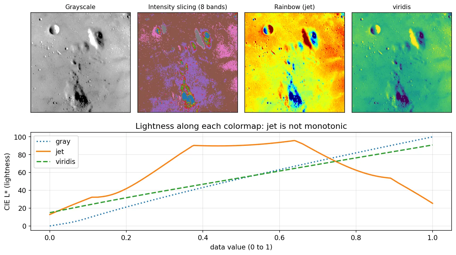
The choice of $T_R, T_G, T_B$ matters more than it looks. The popular rainbow map (jet) passes through bright yellow and cyan in the middle and gets darker at both ends. Its lightness is not monotonic: equal steps in data produce unequal visible steps, flat bands look like edges, and real edges can vanish. Kovesi [7] shows that some widely used maps have perceptual “flat spots” that can hide a feature as large as a tenth of the data range, and argues that a colormap should be designed so that lightness changes uniformly.

viridis, designed by van der Walt and Smith and now Matplotlib’s default [8], was built to be perceptually uniform in the CAM02-UCS color-appearance space, to stay uniform when printed in grayscale, and to remain readable for common forms of color-vision deficiency. Crameri, Shephard and Heron [9] make the same case across the sciences: rainbow and red–green maps distort data and exclude the roughly 8% of men with color-vision deficiency.

import numpy as np
import matplotlib.pyplot as plt
from skimage import data, util, color

g = util.img_as_float(data.moon())
# intensity slicing into 8 equal bands
bands = np.digitize(g, np.linspace(0, 1, 9)[1:-1])          # 0..7
palette = plt.get_cmap("tab10")(np.arange(8))[:, :3]
sliced = palette[bands]                                      # (H, W, 3)
# continuous intensity-to-color transformation
rgb = plt.get_cmap("viridis")(g)[..., :3]
# check a colormap's lightness profile
L = color.rgb2lab(plt.get_cmap("jet")(np.linspace(0, 1, 256))[None, :, :3])[0, :, 0]
print(np.all(np.diff(L) >= 0))                               # False: jet is not monotonic

Rule of thumb: use a sequential uniform map (such as viridis) for ordered data, a diverging map when a meaningful midpoint exists (zero, a threshold), a cyclic map for angles and hue, and a qualitative palette only for unordered categories, as in intensity slicing.

Basics of full-color image processing

In plain words. You can process a color image as three separate gray images, or treat each pixel as a little arrow in color space and process the arrows. Sometimes both give the same answer; often they do not.

A full-color pixel is the vector

$$\mathbf{c}(x, y) = \begin{bmatrix} c_R(x, y) \\ c_G(x, y) \\ c_B(x, y) \end{bmatrix} = \begin{bmatrix} R(x, y) \\ G(x, y) \\ B(x, y) \end{bmatrix}.$$

There are two ways to process it.

1. Per-channel (componentwise). Apply a grayscale method to each channel independently and restack.
2. Vector processing. Work directly on the vectors $\mathbf{c}(x,y)$ using operations that treat the three components together, such as vector distances, vector medians or the color gradient.

Per-channel processing gives the same result as vector processing when two conditions hold: the operation is applicable to both scalars and vectors, and it acts on each component in the same way without mixing them. Linear neighborhood operations satisfy both. Averaging each channel over a window equals averaging the vectors over that window:

$$\frac{1}{|S_{xy}|}\sum_{(s,t)\in S_{xy}} \mathbf{c}(s,t) = \begin{bmatrix} \frac{1}{|S_{xy}|}\sum R(s,t) \\ \frac{1}{|S_{xy}|}\sum G(s,t) \\ \frac{1}{|S_{xy}|}\sum B(s,t) \end{bmatrix},$$

where $S_{xy}$ is the neighborhood centered at $(x,y)$ and $|S_{xy}|$ its number of pixels. Nonlinear operations break the equivalence. A per-channel median can pick the red value from one pixel, the green from a second and the blue from a third, creating a color that appeared nowhere in the neighborhood. Thresholds, edge detectors and histogram equalization are other cases where the vector view matters, as later sections show.

Color transformations

In plain words. A color transformation is a recipe that changes each pixel’s color using only that pixel: make it darker, flip it to its opposite, warm it up, or keep it only if it is “orange enough”.

Formulation

As in Chapter 3, a point transformation is $g(x, y) = T[f(x, y)]$, but now $f$ and $g$ are color vectors. Written per component,

$$s_i = T_i(r_1, r_2, \dots, r_n), \qquad i = 1, \dots, n,$$

where $r_i$ and $s_i$ are the $i$-th input and output components and $n$ is the number of components ($n=3$ for RGB and HSI, $n=4$ for CMYK). Each output may depend on all inputs.

Any effect can be written in any model, but the cost differs. Scaling intensity by $k$ is one multiplication in HSI ($s_3 = k\,r_3$), three in RGB ($s_i = k\,r_i$), and an affine map in CMY ($s_i = k\,r_i + (1-k)$). Pick the model where the operation is natural, but remember that conversions cost time and amplify noise in dark or gray pixels, where hue and saturation are unstable.

Color complements

Hues opposite each other on the color circle are complements: red and cyan, green and magenta, blue and yellow. In RGB the complement is the photographic negative,

$$s_i = 1 - r_i, \qquad i = R, G, B,$$

which is the color version of the gray-level negative in Chapter 3. In HSI the hue complement is $H \mapsto (H + 180^\circ) \bmod 360^\circ$, but the RGB negative also inverts intensity, so it cannot be computed from hue alone. Complements help reveal detail in dark regions.

Color slicing

Color slicing is intensity slicing for color: keep pixels whose color is close to a prototype $\mathbf{a} = (a_R, a_G, a_B)$ and push the rest to a neutral color. Two common definitions of “close”:

$$\text{cube:}\quad s_i = \begin{cases} 0.5, & \text{if } |r_j - a_j| > W/2 \text{ for any } j \\ r_i, & \text{otherwise}\end{cases} \qquad\quad \text{sphere:}\quad s_i = \begin{cases} 0.5, & \text{if } \|\mathbf{r} - \mathbf{a}\| > R_0 \\ r_i, & \text{otherwise}\end{cases}$$

$W$ is the width of a cube centered at $\mathbf{a}$, $R_0$ the radius of a sphere, $\mathbf{r}$ the input color vector and $0.5$ a mid-gray. The sphere treats all directions equally; the cube is cheaper and easy to reason about per channel. A friendlier variant keeps unmatched pixels as their own gray value instead of a flat gray, so context remains visible.

import numpy as np
from skimage import data, util, color

img = util.img_as_float(data.astronaut())
a = np.array([0.85, 0.40, 0.20])            # prototype: the orange of the suit
d = np.linalg.norm(img - a, axis=-1)        # distance of every pixel to a
gray = color.gray2rgb(color.rgb2gray(img))
sliced = np.where((d <= 0.25)[..., None], img, gray)
print((d <= 0.25).mean())                   # fraction kept, about 0.165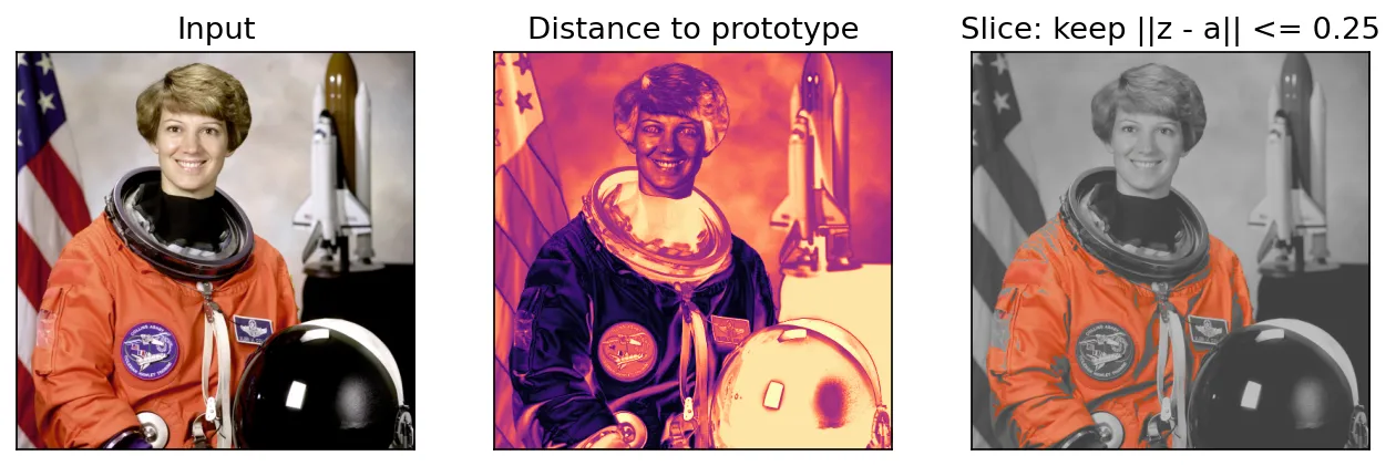

Tone and color corrections

Tone corrections adjust brightness and contrast and are best applied to an intensity-like channel ($I$, $V$ or $L^*$) so hues are preserved. A mostly bright (high-key) image needs a curve that expands the highlights, a dark (low-key) image one that lifts the shadows, a flat image an S-curve.

Color balance corrections remove casts: to reduce a color, add its complement or reduce its neighbors on the color circle. Too much cyan? Increase red, or decrease blue and green. A gray card in the scene gives a precise target: after correction its R, G and B should be equal.

Real workflows convert each device’s colors through a calibrated profile into a device-independent space such as L*a*b*, so a color looks the same on screen and on paper; colors outside a device’s gamut (Figure 6.1) must be mapped inward.

White balance

White balance is the most common automatic color correction. A camera records surface color multiplied by the color of the light, so the same white wall looks orange under tungsten bulbs and bluish in shade. Our visual system largely discounts the light (color constancy); a camera has to do it computationally.

The standard model is diagonal: for illuminant color $\mathbf{e} = (e_R, e_G, e_B)$, the observed pixel is $c_i = e_i\,\rho_i$, where $\rho_i$ is the surface’s response under white light. Correction divides by the estimated illuminant, $\hat\rho_i = c_i / \hat e_i$ (usually rescaled to keep overall brightness). The hard part is estimating $\hat{\mathbf e}$ from one image. Classical estimators make an assumption about the scene:

• Gray world [10]: the average reflectance in a scene is achromatic, so $\hat{\mathbf e} \propto$ the mean RGB of the image.
• White patch (max-RGB) [11], [14]: the brightest surface is white, so $\hat{\mathbf e} \propto$ the per-channel maximum (in practice a high percentile, to ignore a few clipped pixels).
• Gray edge [11]: the average edge (image derivative) is achromatic. Van de Weijer, Gevers and Gijsenij show that all three are members of one family,

$$\left( \int \left| \frac{\partial^n \mathbf{c}_\sigma(\mathbf x)}{\partial \mathbf x^n} \right|^p d\mathbf x \right)^{1/p} = k\,\hat{\mathbf e},$$

applied per channel, where $\mathbf c_\sigma$ is the image smoothed with a Gaussian of scale $\sigma$, $n$ the derivative order, $p$ a Minkowski norm and $k$ a constant. $n=0, p=1$ gives gray world; $n=0, p=\infty$ gives max-RGB; $n=1$ gives gray-edge.

import numpy as np
from skimage import data, util

def white_balance(img, method="gray-world", p=99.5):
    """Diagonal white balance. img: float RGB in [0, 1]."""
    px = img.reshape(-1, 3)
    e = px.mean(0) if method == "gray-world" else np.percentile(px, p, axis=0)
    gain = e.mean() / e                 # one gain per channel
    return np.clip(img * gain, 0, 1), e

img = util.img_as_float(data.astronaut()) * 0.8
biased = np.clip(img * [0.75, 0.95, 1.25], 0, 1)      # add a bluish cast
fixed, e = white_balance(biased, "white-patch")
print(e.round(3))                                      # [0.598 0.757 0.996]

Drag the slider to compare the bluish input with the white-patch correction.

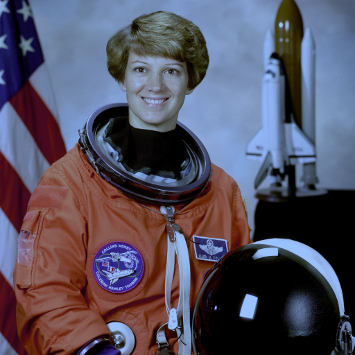
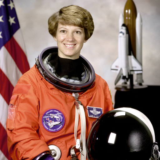Bluish castWhite-patch corrected

Every one of these assumptions fails on some scene. On the cat photo below, whose true average color is orange-brown, gray world “corrects” the warm fur toward gray and leaves a blue tint, while white patch, helped by the white whiskers and highlights, does much better. The angular error between the estimated and true illuminant (the standard metric in this field) is printed above each result.

Histogram processing of color images

Equalizing the R, G and B histograms independently usually produces wrong colors, because it changes the ratios between channels and therefore the hue. The safer approach is to equalize only an intensity channel and leave chromaticity alone:

1. Convert to a model that separates brightness (HSI, HSV, or L*a*b*).
2. Equalize $I$ (or $V$, or $L^*$) using the Chapter 3 method.
3. Convert back.

import numpy as np
from skimage import data, util, exposure, color

img = util.img_as_float(data.astronaut())
per_channel = np.stack([exposure.equalize_hist(img[..., k]) for k in range(3)], -1)  # shifts hues
lab = color.rgb2lab(img)
lab[..., 0] = 100 * exposure.equalize_hist(lab[..., 0] / 100)                      # lightness only
better = np.clip(color.lab2rgb(lab), 0, 1)

Hue is preserved, but some colors may look washed out or leave the gamut on the way back, so a clip or mild saturation boost is sometimes needed. Local histogram methods (Chapter 3) apply to $L^*$ the same way.

Color image smoothing and sharpening

In plain words. To blur or sharpen a color photo you can blur or sharpen each of the three channels, because these are linear operations. But doing it on brightness only is often cleaner.

Smoothing

Neighborhood averaging of a color image is

$$\bar{\mathbf c}(x, y) = \frac{1}{K} \sum_{(s,t) \in S_{xy}} \mathbf c(s, t),$$

where $S_{xy}$ is the neighborhood and $K$ its size. As shown earlier, this equals averaging each channel separately, so cv2.GaussianBlur on a 3-channel array does the right thing.

An alternative is to smooth only the intensity of an HSI (or $L^*$) image and keep hue and saturation. The results differ near edges: per-channel smoothing creates intermediate colors along a red–green boundary (an olive line), while intensity-only smoothing keeps the original hues and only softens brightness. Which you want depends on the task: denoising usually prefers smoothing chroma more than luma, since the eye is less sensitive to chroma blur (the same fact that YCbCr subsampling exploits).

Sharpening

The Laplacian of a vector is the vector of the Laplacians of its components:

$$\nabla^2 \mathbf c(x, y) = \begin{bmatrix} \nabla^2 R(x, y) \\ \nabla^2 G(x, y) \\ \nabla^2 B(x, y) \end{bmatrix},$$

so Laplacian sharpening, $\mathbf g = \mathbf c - k\,\nabla^2 \mathbf c$ with strength $k > 0$, can be done per channel. Unsharp masking (Chapter 3) works the same way. In practice sharpening only the intensity channel avoids colored halos (“fringes”) around high-contrast edges, which appear when the three channels overshoot by different amounts.

Using color in image segmentation

In plain words. Color is one of the easiest clues for splitting an image into parts: “everything brown is stained tissue, everything blue is background.” The question is how to measure “brown enough”.

Segmentation in HSI space

If the target is described by its hue, HSI is a natural choice. A typical recipe: threshold saturation to build a mask of pixels that actually have a color (hue is meaningless at low saturation), multiply the hue image by this mask, then threshold or histogram the masked hue to pick the target range. The weakness is the hue singularity: noise in near-gray pixels produces random hues, which is why the saturation mask comes first.

Segmentation in RGB vector space

RGB vectors often give better results because they avoid the unstable hue computation. Choose a set of sample pixels from the target, compute their mean color $\mathbf a$, and classify every pixel $\mathbf z$ by its distance to $\mathbf a$. The Euclidean distance is

$$D(\mathbf z, \mathbf a) = \|\mathbf z - \mathbf a\| = \left[ (\mathbf z - \mathbf a)^{\mathsf T} (\mathbf z - \mathbf a) \right]^{1/2},$$

and pixels with $D \le D_0$ are labeled as target. The set $D \le D_0$ is a solid sphere of radius $D_0$. Sample colors, however, usually spread more in some directions than others (for stained tissue, mostly along the light-to-dark direction). The Mahalanobis distance accounts for that:

$$D(\mathbf z, \mathbf a) = \left[ (\mathbf z - \mathbf a)^{\mathsf T} \mathbf C^{-1} (\mathbf z - \mathbf a) \right]^{1/2},$$

where $\mathbf C$ is the $3\times3$ covariance matrix of the samples. Now $D \le D_0$ is an ellipsoid aligned with the data. A cheaper approximation is a bounding box centered at $\mathbf a$ whose half-width along each axis is a multiple of that channel’s standard deviation; testing a box needs only comparisons, no squares or square roots.

import numpy as np
from skimage import data, util

img = util.img_as_float(data.immunohistochemistry())
samples = img[60:100, 60:100].reshape(-1, 3)        # a brown (stained) region
a, C = samples.mean(0), np.cov(samples.T)
z = img.reshape(-1, 3) - a
d_euc = np.sqrt((z ** 2).sum(1)).reshape(img.shape[:2])
d_mah = np.sqrt(np.einsum("ij,jk,ik->i", z, np.linalg.inv(C), z)).reshape(img.shape[:2])
mask_euc, mask_mah = d_euc <= 0.25, d_mah <= 3.0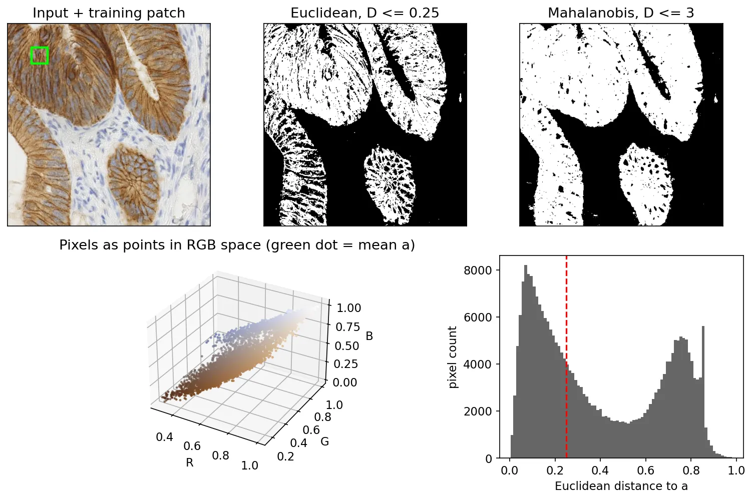

Color edge detection

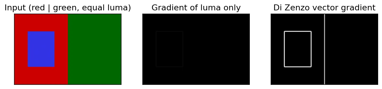
Computing a gradient on each channel and adding the results is a common shortcut, but it is not the gradient of the vector image. Worse, edge detection on a grayscale version misses isoluminant edges, boundaries between two colors of the same brightness. Di Zenzo [13] defined a proper gradient for multi-channel images. With $\mathbf u = (\partial R/\partial x, \partial G/\partial x, \partial B/\partial x)$ and $\mathbf v = (\partial R/\partial y, \partial G/\partial y, \partial B/\partial y)$, define

$$g_{xx} = \mathbf u \cdot \mathbf u, \qquad g_{yy} = \mathbf v \cdot \mathbf v, \qquad g_{xy} = \mathbf u \cdot \mathbf v .$$

These form the $2\times2$ structure tensor $\begin{bmatrix} g_{xx} & g_{xy} \\ g_{xy} & g_{yy} \end{bmatrix}$. The direction of maximum change and the rate of change in that direction are

$$\theta(x, y) = \frac12 \tan^{-1}\!\left( \frac{2 g_{xy}}{g_{xx} - g_{yy}} \right), \qquad F_\theta(x, y) = \left\{ \frac12 \Big[ (g_{xx} + g_{yy}) + (g_{xx} - g_{yy}) \cos 2\theta + 2 g_{xy} \sin 2\theta \Big] \right\}^{1/2}.$$

$\theta$ is the gradient direction (use arctan2 and also test $\theta + 90^\circ$, since the formula gives both extrema), and $F_\theta$ the edge strength. Equivalently, $F_\theta^2$ is the largest eigenvalue of the structure tensor, $\lambda_{\max} = \tfrac12\big[g_{xx} + g_{yy} + \sqrt{(g_{xx} - g_{yy})^2 + 4 g_{xy}^2}\big]$, which is the numerically safer way to compute it.

import numpy as np
from skimage import filters

def di_zenzo(img):
    """Edge strength of a float RGB image via the largest structure-tensor eigenvalue."""
    gx = np.stack([filters.sobel_v(img[..., k]) for k in range(3)], -1)   # d/dx
    gy = np.stack([filters.sobel_h(img[..., k]) for k in range(3)], -1)   # d/dy
    gxx, gyy, gxy = (gx * gx).sum(-1), (gy * gy).sum(-1), (gx * gy).sum(-1)
    return np.sqrt(0.5 * (gxx + gyy + np.sqrt((gxx - gyy) ** 2 + 4 * gxy ** 2)))

Noise in color images

In plain words. Each color channel gets its own noise. When you turn the noisy channels back into hue and saturation, the noise mixes and can look much worse, especially in dark or gray areas.

The noise models of Chapter 5 apply to each channel. In a camera, noise arises mostly in the sensor, before color is reconstructed. Most sensors sit behind a color filter array, so each photosite measures one color and the other two are interpolated (demosaicking); the interpolation spreads and correlates noise across channels. Lukac et al. [12] review this whole chain.

Two observations shape practice:

• Color conversions redistribute noise. Intensity $I = (R+G+B)/3$ averages three channels, so independent zero-mean noise with variance $\sigma^2$ per channel becomes $\sigma^2/3$ in $I$: intensity is cleaner than any channel. Hue and saturation, in contrast, are nonlinear functions with large derivatives near the gray axis, so they become much noisier. This is why denoisers often work in a luma–chroma space and smooth chroma more strongly.
• Impulse noise in one channel is a colored speck. A “salt” spike in the green channel alone makes a bright green dot. A per-channel median removes it, but in mixed cases can create colors that were not in the neighborhood.

The vector median filter avoids invented colors. In each window it outputs the input vector that minimizes the sum of distances to all other vectors in the window [12]:

$$\mathbf c_{\text{VM}} = \arg\min_{\mathbf c_i \in W} \sum_{\mathbf c_j \in W} \|\mathbf c_i - \mathbf c_j\| ,$$

where $W$ is the set of color vectors in the window. The output is always one of the inputs, and for one-dimensional data it reduces to the ordinary median.

import numpy as np
from skimage import data, util

def vector_median(img, k=3):
    r = k // 2
    H, W, _ = img.shape
    p = np.pad(img, ((r, r), (r, r), (0, 0)), mode="edge")
    nb = np.stack([p[i:i + H, j:j + W] for i in range(k) for j in range(k)], 2)  # (H, W, k*k, 3)
    D = np.linalg.norm(nb[:, :, :, None] - nb[:, :, None, :], axis=-1).sum(-1)    # (H, W, k*k)
    return np.take_along_axis(nb, D.argmin(-1)[..., None, None], 2)[:, :, 0]

img = util.img_as_float(data.astronaut())
rng = np.random.default_rng(0)
noisy = img.copy()
hit = rng.random(img.shape[:2]) < 0.05
noisy[hit] = rng.random((hit.sum(), 3))          # 5% random color impulses
out = vector_median(noisy)
psnr = lambda x: 10 * np.log10(1 / ((x - img) ** 2).mean())
print(round(psnr(noisy), 1), round(psnr(out), 1))  # about 20.4 -> 31.3 dB

This vectorized form uses memory proportional to $k^4$ per pixel; use a loop for large windows.

Color image compression

In plain words. A color image has three times the data of a gray one, but much is redundant: the channels look alike, and our eyes see little color detail. Codecs exploit both facts:

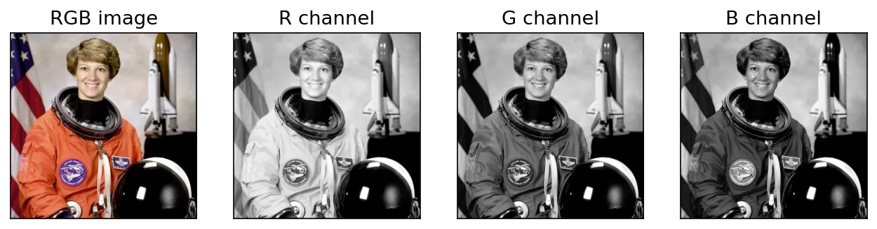
1. Decorrelate the channels. R, G and B are strongly correlated (Figure 6.2 shows three very similar images). Converting to luma plus two chroma differences, such as YCbCr [6], concentrates most of the energy in one channel.
2. Subsample chroma. Because the eye resolves less color detail than brightness detail, the chroma channels can be stored at half resolution horizontally (4:2:2) or in both directions (4:2:0) with little visible loss. 4:2:0 alone halves the raw data: $1 + 2 \cdot \tfrac14 = 1.5$ samples per pixel instead of 3.

Each channel is then compressed with the transform, quantization and entropy coding methods of Chapter 8. Typical color artifacts are bleeding across sharp edges (from chroma subsampling) and blocky color patches at high compression.

Modern view

The classical tools above still run inside every camera and image library. What changed after about 2010 is mostly how the parameters are chosen: learned from data instead of fixed by assumption. Five reviews and survey-style papers map the territory.

Color constancy: from assumptions to learning. Gijsenij, Gevers and van de Weijer [14] survey computational color constancy and sort methods into static methods with fixed assumptions (gray world, white patch, gray edge and the Minkowski family above), gamut-based methods that compare the observed colors with those seen under a canonical light, and learning-based methods trained on images with known illuminants. They also propose comparison criteria and benchmark public algorithms on public datasets; a recurring finding is that no single fixed assumption suits every scene. Learning took over afterwards. Fast Fourier Color Constancy (FFCC) [15] turns illuminant estimation into finding a peak in a log-chroma histogram, solved in the frequency domain; it returns a full distribution over illuminants and runs in real time on phones, which allows temporally smooth auto white balance in video. FC4 [16] is a fully convolutional network in which every patch votes for the illuminant with a learned confidence, so a plain wall counts less than a face or a white object. Afifi and Brown [17] correct white balance after the camera has already rendered a nonlinear sRGB image, which the diagonal model cannot do: their network re-renders the image under other white-balance settings. The diagonal model is still the backbone; the estimate and the corrections in rendered space are now learned.

Vector filtering for color. Lukac et al. [12] review filters that treat color pixels as vectors: vector median and vector directional filters, their variants, vector edge detectors, and demosaicking. Their takeaway matches this chapter: componentwise processing ignores inter-channel correlation and can create color artifacts, while vector order statistics keep the input’s colors. Learned denoisers are now stronger when training data and compute are available, but these filters remain standard baselines where speed and predictability matter.

Colormap design. Kovesi [7] gives a design method and test images for linear, diverging, rainbow and cyclic colormaps, built on one principle: perceived lightness must change uniformly along the map. The viridis family [8] became Matplotlib’s default in version 2.0. Crameri et al. [9] review how color is used across scientific publishing and argue that non-uniform and red–green maps should disappear from software defaults. Deep learning changed nothing here: the problem is human perception, and the answer is careful design measured in a perceptual color space.

Colorization with deep learning. Pseudocolor maps gray to color by a fixed rule; colorization tries to predict the true colors. Zhang, Isola and Efros [18] treat it as classification over quantized colors and rebalance rare classes so that vivid colors are not averaged into brown; they evaluate with a “colorization Turing test” in which people judge whether an image is real. Anwar et al. [19] survey deep colorization, group methods into seven categories, discuss losses and metrics, and introduce a new benchmark dataset. DDColor [20] (ICCV 2023) uses two decoders, one restoring spatial detail and one refining color with cross-attention to multi-scale semantic features, plus a colorfulness loss; this reduces color bleeding across object boundaries. Two classical ideas persist: work in L*a*b* (predict chroma, keep the given lightness) and treat color as a distribution, because a gray shirt could have been any color.

What did not change. Colorimetry (CIE XYZ, chromaticity, gamuts), encodings (sRGB, BT.601/709 YCbCr) and color-difference spaces are standards, not things to learn. Networks are trained on sRGB data and judged in these spaces. Knowing exactly which space your tensors are in (encoded or linear, BT.601 or BT.709, studio or full range) remains one of the most practical skills in color work.

Key takeaways

• Human vision is trichromatic, so three numbers describe a color for a human observer; different spectra with equal responses (metamers) look the same.
• The CIE xy chromaticity diagram shows all visible chromaticities; a three-primary device covers only a triangle (its gamut).
• RGB suits hardware, CMY(K) suits ink, HSI separates intensity from hue and saturation, and L*a*b* makes Euclidean distance roughly perceptual. Watch for undefined hue on grays, sRGB gamma, and BT.601 versus BT.709.
• Pseudocolor makes gray data readable; use perceptually uniform colormaps such as viridis, not rainbow maps.
• Linear operations (smoothing, Laplacian sharpening) can be done per channel; nonlinear ones (median, histogram equalization, edge detection, segmentation) should treat pixels as vectors or work on an intensity channel.
• White balance divides by an estimated illuminant; gray world, white patch and gray edge are special cases of one framework, and modern systems learn the estimate.
• Segment color with vector distances (Euclidean, Mahalanobis, box), and detect color edges with the Di Zenzo gradient, which sees isoluminant boundaries.
• Intensity is less noisy than any single channel, hue and saturation are more noisy; vector median filters remove color impulses without inventing new colors.

Exercises

1. A pixel has $(R, G, B) = (0.6, 0.6, 0.2)$. Compute its H, S and I by hand. Then predict, without computing, how H changes if B increases to $0.3$.

Hint

$I = 0.4667$. $\min = 0.2$, so $S = 1 - 0.2/0.4667 \approx 0.571$. For $\theta$: numerator $= 0.5(0 + 0.4) = 0.2$, denominator $= \sqrt{0 + 0.4 \cdot 0.4} = 0.4$, so $\theta = \cos^{-1}(0.5) = 60^\circ$, and since $B \le G$, $H = 60^\circ$ (yellow). Raising B to $0.3$ keeps $R = G$, so hue stays $60^\circ$; only S drops.

2. Show that the RGB negative $s_i = 1 - r_i$ maps a pixel with HSI coordinates $(H, S, I)$ to one whose intensity is $1 - I$ and whose hue is $H + 180^\circ$ (for non-gray pixels). Is the saturation preserved?

Hint

Intensity follows from linearity. For hue, the chromatic part $\mathbf c - I\,\mathbf 1$ simply changes sign, which rotates it by $180^\circ$ around the gray axis. Saturation is $1 - \min/I$; after negation the minimum becomes $1 - \max(R,G,B)$ and the intensity $1 - I$, so in general saturation changes. Try $(0.9, 0.1, 0.1)$.

3. You equalize the R, G and B histograms of a photo of a blue sky separately. Explain why the sky may turn gray-cyan, and propose two fixes.

Hint

Equalization stretches each channel to use the full range. A channel that was almost uniformly high (blue) can be pushed down relative to the others, while weak channels are boosted, so the R:G:B ratio changes. Fix by equalizing $I$, $V$ or $L^*$ only, or by applying one common mapping computed from the average histogram to all three channels.

4. In the gray-world/white-patch framework, what estimator do you get with $n = 0$ and $p = 2$? Run the white_balance idea on the cat image with $p = 1, 2, 6, \infty$ (use a high percentile for $\infty$) and plot the angular error versus $p$.

Hint

$p = 2$ estimates the illuminant from the root-mean-square value of each channel, a compromise between the mean and the maximum. With the chapter’s synthetic cast the error falls from about 12° ($p=1$) to about 11° ($p=2$), 7° ($p=6$) and 4° ($p=20$). It falls as $p$ grows on this image, because its bright white details are a better clue than its orange average. On a scene without white objects the trend can reverse.

5. Design a color segmenter for green vegetation in outdoor photos that is robust to shadows. Which space and which distance would you use, and why might plain RGB Euclidean distance fail?

Hint

Shadows scale all three channels down, which moves a pixel along a line through the origin and changes its RGB Euclidean distance a lot. Use a chromaticity-based feature that is unaffected by scaling (normalized $r = R/(R+G+B)$, $g = G/(R+G+B)$, or hue with a saturation mask, or $a^*, b^*$), or a Mahalanobis distance whose covariance is trained on sunlit and shaded samples.

6. Explain why the vector median filter never creates a new color, and give a $3$-pixel, 1-D example where the per-channel median does.

Hint

By definition the vector median is one of the window’s input vectors. For three pixels $(1,1,0)$, $(1,0,1)$, $(0,1,1)$ (yellow, magenta, cyan) the per-channel median is $(1,1,1)$, pure white, which appears nowhere in the window.

The figures in this chapter are generated by scripts/figures/dip_ch06.py from skimage.data images and synthetic arrays.

References

1. R. C. Gonzalez and R. E. Woods, Digital Image Processing, 4th ed., Pearson, 2018, Ch. 6. publisher page
2. C. Wyman, P.-P. Sloan, and P. Shirley, “Simple Analytic Approximations to the CIE XYZ Color Matching Functions,” Journal of Computer Graphics Techniques, vol. 2, no. 2, 2013. jcgt.org
3. IEC 61966-2-1:1999, “Multimedia systems and equipment – Colour measurement and management – Part 2-1: Colour management – Default RGB colour space – sRGB,” IEC, 1999. IEC webstore
4. Recommendation ITU-R BT.709-6, “Parameter values for the HDTV standards for production and international programme exchange,” ITU, 2015. ITU
5. ISO/CIE 11664-4:2019, “Colorimetry – Part 4: CIE 1976 L*a*b* colour space,” ISO/CIE, 2019. standard page
6. Recommendation ITU-R BT.601-7, “Studio encoding parameters of digital television for standard 4:3 and wide screen 16:9 aspect ratios,” ITU, 2011. ITU
7. P. Kovesi, “Good Colour Maps: How to Design Them,” arXiv:1509.03700, 2015. arXiv
8. S. van der Walt and N. Smith, viridis colormap design notes (BIDS project page; presented at SciPy 2015), 2015. project page
9. F. Crameri, G. E. Shephard, and P. J. Heron, “The misuse of colour in science communication,” Nature Communications, vol. 11, art. 5444, 2020. PMC
10. G. Buchsbaum, “A spatial processor model for object colour perception,” Journal of the Franklin Institute, vol. 310, no. 1, pp. 1–26, 1980. DOI
11. J. van de Weijer, T. Gevers, and A. Gijsenij, “Edge-Based Color Constancy,” IEEE Transactions on Image Processing, vol. 16, no. 9, pp. 2207–2214, 2007. DOI
12. R. Lukac, B. Smolka, K. Martin, K. N. Plataniotis, and A. N. Venetsanopoulos, “Vector Filtering for Color Imaging,” IEEE Signal Processing Magazine, vol. 22, no. 1, pp. 74–86, Jan. 2005. PDF
13. S. Di Zenzo, “A note on the gradient of a multi-image,” Computer Vision, Graphics, and Image Processing, vol. 33, pp. 116–125, 1986. DOI
14. A. Gijsenij, T. Gevers, and J. van de Weijer, “Computational Color Constancy: Survey and Experiments,” IEEE Transactions on Image Processing, vol. 20, no. 9, pp. 2475–2489, 2011. DOI
15. J. T. Barron and Y.-T. Tsai, “Fast Fourier Color Constancy,” CVPR, 2017. arXiv
16. Y. Hu, B. Wang, and S. Lin, “FC4: Fully Convolutional Color Constancy with Confidence-Weighted Pooling,” CVPR, 2017. paper
17. M. Afifi and M. S. Brown, “Deep White-Balance Editing,” CVPR, 2020. arXiv
18. R. Zhang, P. Isola, and A. A. Efros, “Colorful Image Colorization,” arXiv:1603.08511, 2016. arXiv
19. S. Anwar, M. Tahir, C. Li, A. Mian, F. S. Khan, and A. W. Muzaffar, “Image Colorization: A Survey and Dataset,” arXiv:2008.10774, 2020. arXiv
20. X. Kang, T. Yang, W. Ouyang, P. Ren, L. Li, and X. Xie, “DDColor: Towards Photo-Realistic Image Colorization via Dual Decoders,” ICCV, 2023. arXiv