DL 05 · Low-Light Image Enhancement

What you’ll learn

• Why low-light image enhancement (LLIE) is two problems at once, tone enhancement and detail and noise restoration, and why “just make it brighter” fails.
• How the classical toolbox works: brightness channels in HSV, HSI, YCbCr and Lab; histogram equalization and CLAHE; gamma curves; Retinex (SSR, MSR, LIME); and the dehazing-inversion trick.
• How deep LLIE methods are organized by their training signal (supervised, unrolled, unpaired, zero-reference, generative), with the math of the Retinex-Net decomposition losses and the Zero-DCE curve.
• How to evaluate enhancement honestly: full-reference vs. no-reference metrics, the GT-mean pitfall, and task-driven evaluation.
• Which datasets and challenges (LOL, LOL-v2, LSRW, SDSD, SID, FiveK, ExDark, NTIRE 2024/2025) are used for what, and what remains unsolved.

The big picture

A photo taken in the dark is not just a normal photo with the brightness turned down. The sensor collected very few photons, so the picture is dim, noisy, and often has a color cast. Low-light image enhancement aims to produce the image you would have gotten with good light: well exposed, with natural colors, clean details, and no new artifacts.

Why it matters: phones shoot in the dark every day, cars and robots must see at night, and surveillance, astronomy-like scientific imaging and medical endoscopy all fight the same physics. Low light also hurts downstream models: a detector trained on daytime photos loses accuracy at night. That makes LLIE both a picture-quality task and a robustness task for computer vision.

Goal and difficulty

Plain version. We want to map a dark image to a normally exposed one. The hard part is that brightening and repairing are different jobs: brightening changes tone (how light or dark each region is), while repairing recovers details and clean colors that the darkness and noise destroyed.

Precise version. Unlike image-to-image translation, which changes an image’s attributes (summer to winter, photo to painting), LLIE should keep the scene and its content exactly as they are and only undo the damage caused by insufficient light. The post [1] splits that damage into two difficulties:

1. Tone enhancement. Lift the exposure, globally and locally, without crushing highlights or flattening contrast. Bright regions such as lamps must stay bright, dark regions must open up, and the ordering of brightness between regions should be preserved.
2. Detail restoration. Recover texture and color that are buried in noise and quantization, while suppressing that noise rather than amplifying it.

In deep learning, detail restoration is what a network does anyway once it is trained to output a clean image, so most method design goes into the tone part (which image properties or physical model to build in) and the learning mechanism (which supervision and losses to use), rather than into a dedicated detail module.

Why it is not simple brightening

A linear gain $y = c\,x$ with $c > 1$ fails in four ways, all visible in Figure 1:

• Noise. Photon arrival is random. With few photons, the signal-to-noise ratio is low, and a gain multiplies signal and noise equally. The image gets brighter, not cleaner.
• Color cast. Low light is often colored (tungsten, sodium street lamps), and the camera’s white balance and the three color channels have different noise levels. Scaling the channels equally keeps the cast; scaling them separately may produce strange colors.
• Saturation and over-exposure. Pixels already near the top (lamps, windows, screens) clip at 1. A global gain big enough for the shadows destroys the highlights.
• Quantization. A dark 8-bit image may use only 20–40 distinct gray levels. Stretching them produces visible banding.

A model of low-light capture

It helps to have an explicit degradation model, both for understanding and for synthesizing training data. Work in linear light (values proportional to photon counts), not on gamma-encoded pixels (see DIP Chapter 3 on gamma). A widely used model is the Poisson–Gaussian model of Foi et al. [7]:

$$z = \frac{1}{\eta}\,\mathcal{P}\!\left(\eta\,k\,x\right) + n, \qquad n \sim \mathcal{N}(0, \sigma_r^2),$$

where $x \in [0, 1]$ is the clean linear image, $k \in (0, 1]$ the fraction of light that reached the sensor, $\eta$ a scale that converts intensity to photon counts (a larger $\eta$ means more photons and less relative noise), $\mathcal{P}(\cdot)$ a Poisson random variable modeling shot noise, and $n$ Gaussian read noise with standard deviation $\sigma_r$. The camera then applies a tone curve and quantizes. The variance of $z$ is approximately $k x/\eta + \sigma_r^2$: it grows with the signal, so noise is signal-dependent, which is why “add Gaussian noise” is a poor stand-in for real low light.

import numpy as np
from skimage import data, img_as_float

rng = np.random.default_rng(0)
clean = img_as_float(data.coffee())            # H x W x 3, sRGB-encoded, in [0, 1]

def synth_low_light(x, k=0.05, peak=2000.0, read_std=8e-4, gamma=2.2):
    lin = k * x ** gamma                           # 1) less light, in linear units
    lin = rng.poisson(lin * peak) / peak           # 2) shot noise (Poisson)
    lin = lin + rng.normal(0, read_std, lin.shape) # 3) read noise (Gaussian)
    out = np.clip(lin, 0, 1) ** (1 / gamma)        # 4) re-encode for display
    return np.round(out * 255) / 255               # 5) 8-bit quantization

dark = synth_low_light(clean)
print(clean.mean(), dark.mean())                   # about 0.39 -> 0.10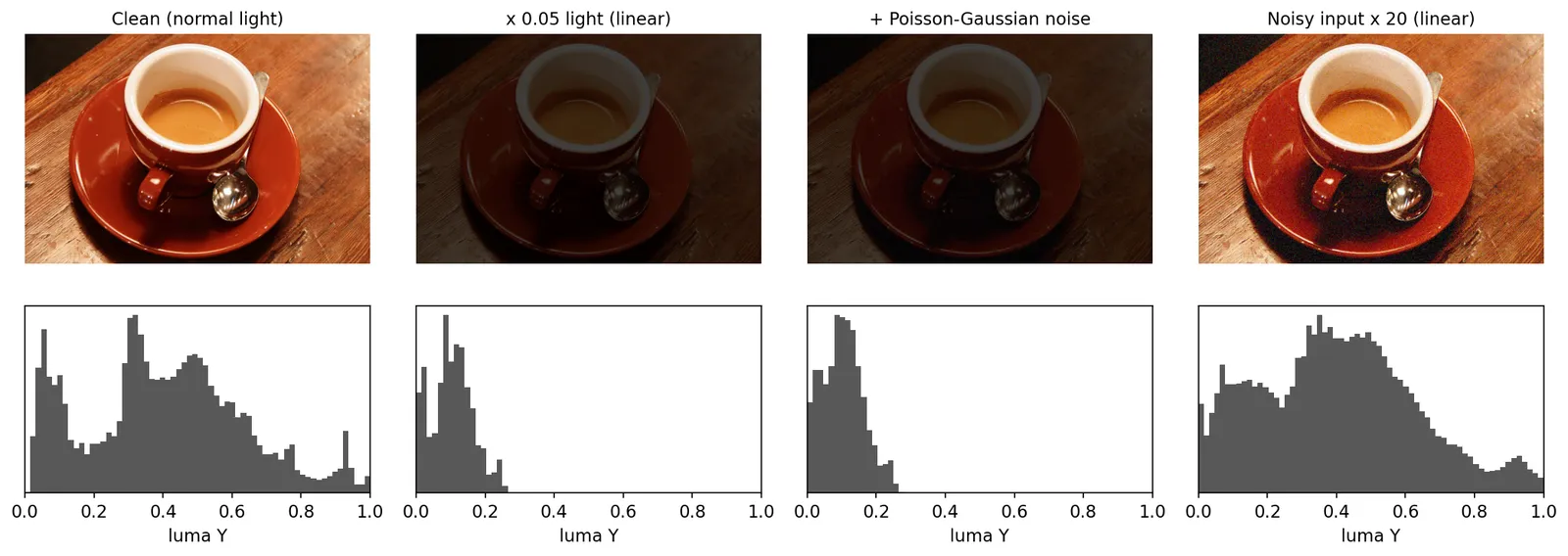

The right panel is the most important picture in this tutorial: even the ideal brightness correction leaves the noise, which is why LLIE is a restoration problem (see DL 04 · Image Restoration) and not only a tone-mapping problem.

Non-deep-learning LLIE and the characteristics of low-light images

Plain version. Before deep learning there were two main families: histogram-based methods, which redistribute gray levels, and Retinex-based methods, which split an image into “lighting” and “objects” and fix the lighting. A third idea, borrowed from dehazing, fits into the Retinex family, and statistical methods extend all of them.

Low-light images in color space

Many color spaces separate a “how bright” channel from “what color” channels. Different spaces call it value, intensity, luma or lightness, and each defines it differently. With $R, G, B \in [0, 1]$ (see DIP Chapter 6 for the spaces themselves):

$$\begin{aligned} \text{HSV:}\quad & V = \max(R, G, B), \\ \text{HSI:}\quad & I = \tfrac{1}{3}(R + G + B), \\ \text{YCbCr (BT.601):}\quad & Y' = 0.299\,R' + 0.587\,G' + 0.114\,B', \\ \text{CIELAB:}\quad & L^{*} = 116\, f\!\left(Y_{\text{lin}}/Y_n\right) - 16 . \end{aligned}$$

Here $R', G', B'$ are gamma-encoded values; $Y_{\text{lin}}$ is linear-light luminance and $Y_n$ that of the reference white; $f(t) = t^{1/3}$ above a small threshold and linear below it. Some remarks:

• $V$ is the “bright channel”. It is the per-pixel maximum, the counterpart of the dark channel (a per-patch minimum) used in dehazing [14]. In a dark image, $V$ is the channel least damaged by the darkness, which is why LIME [17] uses it to initialize the illumination.
• The luma weights. ITU-R BT.601 [8] defines luma as $Y' = 0.299R' + 0.587G' + 0.114B'$. That full-range form is what JPEG/JFIF uses. For 8-bit limited-range (“studio”) video, BT.601 places black at 16 and white at 235: $Y = 16 + 219\,Y'$. With $R', G', B' \in [0, 255]$ this becomes $Y = 16 + 0.257R' + 0.504G' + 0.098B'$, because $219/255 \times (0.299, 0.587, 0.114) \approx (0.257, 0.504, 0.098)$. Both formulas describe the same luma; they differ only in range and offset.
• $L^*$ is designed to be perceptually uniform, so equal steps look roughly equal to a person. That makes it a good channel for contrast enhancement.

The practical lesson: since brightness can be separated from color, you can enhance only the brightness channel and keep the chroma. Figure 2 shows that the choice of channel matters a lot.

R, G, B = dark[..., 0], dark[..., 1], dark[..., 2]
V = dark.max(axis=2)                          # HSV value
I = dark.mean(axis=2)                         # HSI intensity
Y = 0.299 * R + 0.587 * G + 0.114 * B         # BT.601 luma, full range (JPEG/JFIF)
Y_limited = 16 + 219 * Y                      # 8-bit limited ("studio") range, 16..235
print(np.allclose(Y_limited, 16 + (65.481 * R + 128.553 * G + 24.966 * B)))  # True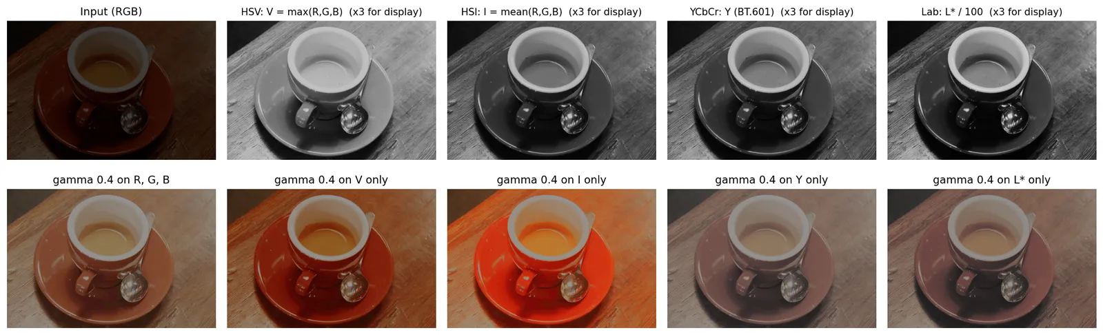

Two effects are visible. Scaling RGB by a common factor (HSV, HSI) preserves hue and keeps the ratio between channels, so saturated objects become very saturated. Changing only $Y'$ or $L^*$ while keeping Cb/Cr or a*/b* fixed adds brightness without adding color, so the image looks washed out. This coupling of tone and color is exactly what later methods such as HVI-CIDNet [27] try to handle with a learned color space.

Histogram equalization and CLAHE

Plain version. Histogram equalization (HE) spreads the gray levels of an image so that all brightness values are used about equally. A dark image, whose values are packed near zero, gets stretched across the full range.

Precise version. For an image with $L$ levels, normalized histogram $p_r(r_k) = n_k / (MN)$, HE uses the scaled cumulative distribution function as the mapping:

$$s_k = T(r_k) = (L - 1) \sum_{j=0}^{k} p_r(r_j), \qquad k = 0, \dots, L - 1,$$

where $n_k$ is the number of pixels at level $r_k$ and $MN$ the image size. The slope of $T$ is proportional to the histogram, so heavily populated gray levels get pulled apart. The derivation is in DIP Chapter 3. For color images, the usual recipe is to convert to a space with a brightness channel, equalize that channel only, and convert back, for example RGB → Lab → equalize $L^*$ → RGB.

Global HE has two problems in low light: it over-stretches large flat regions (including their noise), and one mapping cannot serve both a dark corner and a bright lamp. Adaptive HE computes a mapping per tile, and CLAHE (contrast-limited AHE) clips each tile’s histogram at a limit before computing the CDF, which caps the slope of $T$ and therefore the noise gain, then interpolates between neighboring tiles to avoid seams [9], [10].

Gamma correction

A power law $s = r^{\gamma}$ with $\gamma \lt 1$ lifts shadows more than highlights; its slope $\gamma r^{\gamma - 1}$ is large near $r = 0$. It is cheap and monotonic but global: one $\gamma$ for the whole picture, no denoising, and the same desaturation-or-oversaturation choice as above depending on where it is applied.

from skimage import color, exposure

gamma_out = dark ** 0.4                                     # power-law curve on every channel
lab = color.rgb2lab(dark)
L = lab[..., 0] / 100                                       # L* scaled to [0, 1]
he = lab.copy();    he[..., 0] = 100 * exposure.equalize_hist(L)
clahe = lab.copy(); clahe[..., 0] = 100 * exposure.equalize_adapthist(L, clip_limit=0.01)
he_out, clahe_out = color.lab2rgb(he), color.lab2rgb(clahe)
for name, im in [("gamma", gamma_out), ("HE", he_out), ("CLAHE", clahe_out)]:
    print(f"{name:6s} mean {im.mean():.3f}   std {im.std():.3f}")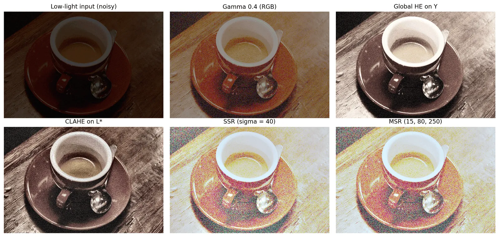

Retinex theory

Plain version. Retinex says that what the eye (or camera) receives is “the object’s own colors” multiplied by “the light falling on it”. If we can estimate the light, we can divide it out and see the object as it really is, then put back a better light.

Precise version. Land’s Retinex theory [11] models an observed image $S$ as

$$S(\mathbf{x}) = R(\mathbf{x}) \circ L(\mathbf{x}),$$

where $\mathbf{x}$ is the pixel position, $R \in [0, 1]$ is the reflectance (a property of the surfaces, assumed constant under any lighting), $L$ is the illumination (the light falling on the scene, which varies smoothly in space except at shadow boundaries), and $\circ$ is element-wise multiplication. Note the word: $L$ is illumination, not luminance. “Luminance” usually refers to a brightness channel of a color space, such as $Y$ above.

Recovering two unknowns from one product is ill-posed, so every Retinex method adds a prior. The classic one is “illumination is smooth”.

Single-scale Retinex (SSR) [12] estimates $L$ with a Gaussian blur $G_\sigma$ and works in the log domain, where the product becomes a sum:

$$\log R_c(\mathbf{x}) = \log S_c(\mathbf{x}) - \log\big(G_\sigma * S_c\big)(\mathbf{x}),$$

for each color channel $c$, with $*$ convolution and $\sigma$ the surround scale. Small $\sigma$ gives strong local contrast and halos at edges; large $\sigma$ gives better tone but weaker detail. Multi-scale Retinex (MSR) [13] averages SSR outputs at several scales (typically three) with weights $w_n$:

$$\log R_c^{\text{MSR}} = \sum_{n=1}^{N} w_n \left[\log S_c - \log(G_{\sigma_n} * S_c)\right].$$

Because SSR and MSR work per channel, they tend to gray out the colors. MSRCR (MSR with color restoration) [13] multiplies the result by a color-restoration factor based on each channel’s share of $R + G + B$; other variants apply MSR to an intensity channel only and keep the input’s chromaticity.

from scipy import ndimage as ndi

def ssr(img, sigma=40.0, eps=1e-3):
    log_s = np.log(img + eps)
    log_l = np.log(ndi.gaussian_filter(img, sigma=(sigma, sigma, 0)) + eps)  # L ~ Gaussian blur
    r = log_s - log_l                                       # log R = log S - log L
    lo, hi = np.percentile(r, [1, 99])                      # robust stretch for display
    return np.clip((r - lo) / (hi - lo), 0, 1)

msr = np.mean([ssr(dark, s) for s in (15, 80, 250)], axis=0)   # MSR, equal weights (simplified)

For enhancement we usually do not want $R$ alone, which looks flat and unnatural. We want to brighten $L$ and recombine: $\hat{S} = R \circ \hat{L}$ with, for example, $\hat{L} = L^{\gamma}$ and $\gamma \lt 1$. This “decompose, adjust $L$, recombine” pattern is the template for most Retinex-based deep networks.

LIME: Retinex as optimization

LIME [17] estimates only the illumination. It initializes it with the bright channel, $\hat{T}(\mathbf{x}) = \max_{c} S_c(\mathbf{x})$, then refines it by solving a structure-aware smoothing problem: keep $T$ close to $\hat{T}$, but make it smooth except where the image has strong structure. The enhanced image is $S / T^{\gamma}$, and because dividing amplifies noise, LIME optionally denoises afterward. LIME’s images (often called the LIME set) became a standard test set, and the method is a good example of the classical recipe: a physical model, a hand-designed prior, and an optimization.

Another model: dehazing an inverted image

The Retinex model is not the only image-formation model. Dehazing uses the atmospheric scattering model:

$$I(\mathbf{x}) = J(\mathbf{x})\, t(\mathbf{x}) + A\,\big(1 - t(\mathbf{x})\big),$$

where $I$ is the hazy observation, $J$ the haze-free scene radiance, $t \in (0, 1]$ the transmission (how much scene light survives), and $A$ the global atmospheric light. This model cannot be applied to a dark image directly, because a dark image does not look like a hazy one.

Dong et al. observed that an inverted low-light image, $1 - S$, does look hazy: dark regions become bright and low-contrast, like fog. They therefore invert the image, run a dehazing algorithm (in the spirit of the dark channel prior [14]), and invert the result back [15], [16]. In the notation above,

$$I_{\text{haze}} = 1 - S_{\text{Retinex}}, \qquad J_{\text{haze}} = 1 - \hat{S}_{\text{enhanced}} .$$

From the “what is reliable” angle, dehazing assumes the dark channel marks haze-free content; in a low-light image the dark channel is mostly damaged pixels, so attention shifts to the bright channel, the region least affected by the darkness. The LIME paper [17] analyzes this inversion approach and shows that it can be rewritten in Retinex form, so the two models make essentially the same assumption, with Retinex being the simpler statement.

Statistical approaches

Many classical methods add statistics or priors on top of these models: naturalness constraints that keep the lightness order of a scene (NPE [18]), layered or two-dimensional histogram models (the method behind the DICM set [59]), and fusion of several synthetic exposures. They are hand-crafted, need no training data, and generalize in a predictable way; their weak point is noise, which they usually ignore or hand to a separate denoiser.

Deep-learning LLIE

Plain version. Deep networks learn the mapping from dark to bright from data. The question is not whether to use a network but what training signal to use: paired dark/bright photos, unpaired photos, no reference at all, or a generative model of what bright images look like. Physics (usually Retinex) can be built into any of these.

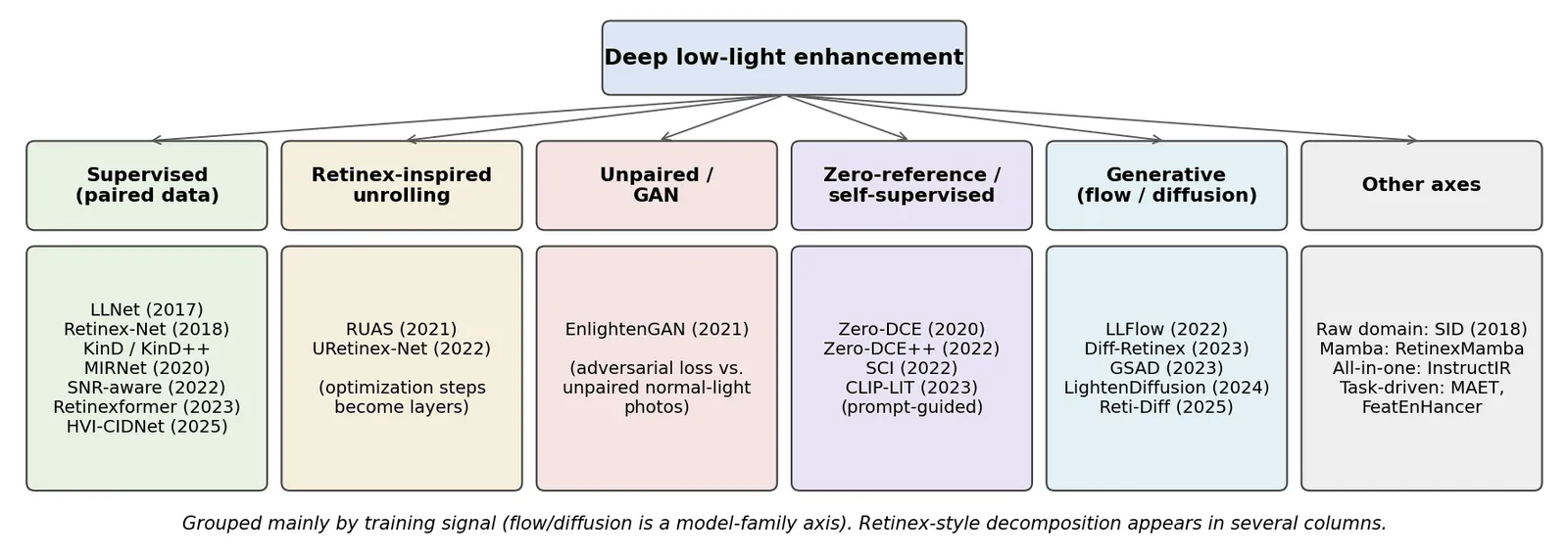
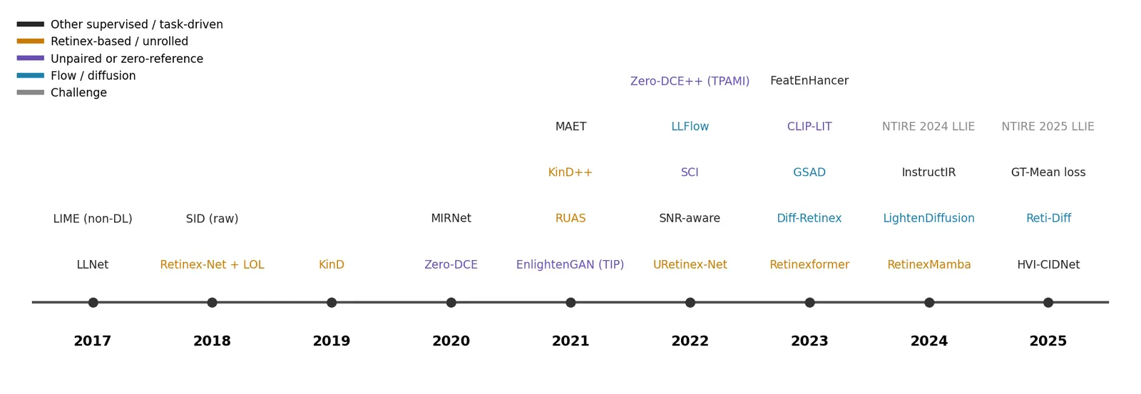
Deep learning is itself a large optimization, and its black-box nature lets us drop many hand-made assumptions. A common first split is theory-based methods (usually Retinex) versus theory-free methods (strong generic networks). In practice the two mix, so the split is not binary. Figure 5 groups methods mainly by training signal instead, following the surveys [2], [3].

Supervised methods (paired data)

Given pairs $(x_i, y_i)$ of low-light and normal-light images, train $f_\theta$ to minimize a reconstruction loss, typically $\mathcal{L} = \lVert f_\theta(x) - y\rVert_1$ plus perceptual or structural terms. Paired data is expensive (two exposures of a static scene, or synthesis), and the network learns the specific brightness and color style of the reference images, which matters for evaluation later.

• LLNet [19] (2017) was one of the first deep LLIE models: a stacked sparse denoising autoencoder trained on synthetically darkened and noised patches, learning brightening and denoising jointly.
• CNN + bright channel prior (Tao et al. [20], 2017) handled the two difficulties in sequence: a CNN denoises first, then contrast is enhanced with an atmospheric-scattering-style model driven by the bright channel, an early example of combining learning with the inversion idea above.
• MIRNet [24] (2020) is a general restoration backbone that keeps a full-resolution stream alongside parallel lower-resolution streams, exchanges information between them, fuses them with selective-kernel attention, and was evaluated on enhancement as well as denoising and super-resolution.
• SNR-aware [25] (2022) estimates a per-pixel signal-to-noise map. Where SNR is high, local convolution is enough; where SNR is very low, the local neighborhood is unreliable, so the model uses long-range transformer attention to borrow information from elsewhere in the image.
• HVI-CIDNet [27] (2025) attacks the color-space problem of Figure 2: sRGB is very sensitive to color and gives color bias and brightness artifacts, and HSV fixes brightness but creates red and black noise. The authors propose the HVI space, built from polarized hue/saturation maps and a learnable intensity, plus a network that decouples color and intensity.

Retinex-based networks

Retinex-Net [21] (2018) changed the goal from “estimate $R$” to “both the input and the output have their own $R$ and $L$”. The pipeline is: decompose the low and normal images, enhance $L$ to $\hat{L}$, recombine with $R$. It also introduced the LOL dataset (below). Its decomposition network is trained only through consistency, without ground-truth $R$ or $L$, using

$$\mathcal{L}_{\text{decom}} = \mathcal{L}_{\text{recon}} + \lambda_{ir}\,\mathcal{L}_{ir} + \lambda_{is}\,\mathcal{L}_{is},$$ $$\mathcal{L}_{\text{recon}} = \sum_{i \in \{\text{low},\text{normal}\}} \sum_{j \in \{\text{low},\text{normal}\}} \lambda_{ij} \left\lVert R_i \circ I_j - S_j \right\rVert_1,$$ $$\mathcal{L}_{ir} = \lVert R_{\text{low}} - R_{\text{normal}} \rVert_1, \qquad \mathcal{L}_{is} = \sum_{i} \left\lVert \nabla I_i \circ \exp\!\left(-\lambda_g \nabla R_i\right) \right\rVert .$$

In the paper’s notation $S = R \circ I$, so $I$ here is the illumination ($L$ in our notation). $S_j$ is the input image $j$, $R_i$ and $I_i$ the decomposed reflectance and illumination of image $i$, and $\nabla$ the horizontal plus vertical gradient. The terms say:

• $\mathcal{L}_{\text{recon}}$: each decomposition must reproduce its own image ($\lambda_{ii} = 1$), and crossing reflectance and illumination between the pair should still roughly work ($\lambda_{ij} = 0.001$ for $i \neq j$).
• $\mathcal{L}_{ir}$: the two images show the same scene, so their reflectances should be equal; this is how the network learns what “reflectance” means.
• $\mathcal{L}_{is}$: illumination should be smooth, except where the reflectance has a strong edge. The weight $\exp(-\lambda_g \nabla R)$ relaxes the smoothness penalty across object boundaries. This is the learned version of LIME’s structure-aware prior.

The paper uses $\lambda_{ir} = 0.001$, $\lambda_{is} = 0.1$ and $\lambda_g = 10$. The enhancement network is trained with $\lVert R_{\text{low}} \circ \hat{I} - S_{\text{normal}} \rVert_1$ plus the same smoothness term.

The pattern spread quickly, and many names contain “Retinex”:

• KinD [22] (2019) splits the work into three subnetworks: decomposition, reflectance restoration (because the dark image’s reflectance is noisy and color-shifted, the “R is unchanged” assumption is relaxed), and illumination adjustment with a user-controllable brightness ratio. KinD++ [23] (2021) refines the design to reduce visual defects.
• Retinexformer [26] (2023) notes that both capture and brightening corrupt the components, and rewrites the model with perturbations: $S = (R + \hat{R}) \circ (L + \hat{L})$, where $\hat{R}$ and $\hat{L}$ model noise, artifacts and color distortion. It is trained in one stage (instead of Retinex-Net’s multi-stage training) with an L1 loss, and its illumination-guided multi-head self-attention uses the illumination estimate to steer attention, so regions with different exposure interact. It became a common baseline.
• RetinexMamba [42] (2024 preprint) keeps the Retinex-transformer structure and replaces attention with Mamba state-space blocks, which scale linearly with the number of pixels. “Retinex decomposition plus a new backbone” has been a stable design pattern for years.

A less common route builds on the atmospheric scattering model rather than plain Retinex. CPGA-Net [28] combines channel priors with gamma correction in a lightweight network that processes global and local information, and CPGA-Net+ [29] revisits the theoretical illumination model for efficiency. That line of work also reports that the features learned by different functional modules follow the physical roles of the priors, which suggests that a network guided by a model is not a completely opaque black box.

Retinex-inspired unrolling

Unrolling (or unfolding) takes an iterative optimization algorithm for the Retinex problem and turns each iteration into a network stage with learnable parameters. The architecture inherits the algorithm’s structure and interpretability, and training replaces hand-tuned priors.

• RUAS [30] (2021) unrolls optimization models for illumination estimation and noise removal, searches the architecture of the prior modules, and is trained with a cooperative reference-free strategy, so it also belongs in the unsupervised column. It is very small and fast.
• URetinex-Net [31] (2022) unfolds a Retinex decomposition optimization into a network with learned modules for initialization, the unfolded updates of $R$ and $L$, and illumination adjustment.

Unpaired training: EnlightenGAN

EnlightenGAN [32] (2021) uses a generative adversarial network (GAN) so that it needs only a set of dark images and an unrelated set of well-lit images. A U-Net generator, guided by a self-regularized attention map derived from the input’s illumination, produces the enhanced image. A global discriminator judges the whole image and a local discriminator judges random patches, so the output looks like a well-lit photo both overall and in detail. A self-feature-preserving loss compares VGG features of input and output, keeping content in place since there is no ground truth to do so.

Zero-reference methods and curve estimation

Plain version. Zero-DCE does not output a new image. It outputs a brightening curve per pixel, applies it, and is trained with losses that judge the result without any reference photo: “is it well exposed, is the color balanced, is the curve smooth, is local contrast kept?”

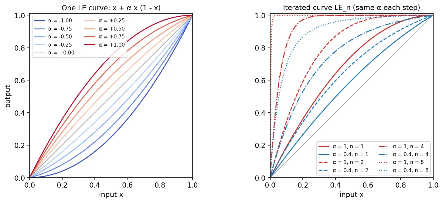
The LE curve. Zero-DCE [33] (2020) defines a quadratic light-enhancement curve

$$\mathrm{LE}(x;\alpha) = x + \alpha\, x\,(1 - x), \qquad \alpha \in [-1, 1],$$

where $x \in [0, 1]$ is a pixel value. The curve has three useful properties: $\mathrm{LE}(0) = 0$ and $\mathrm{LE}(1) = 1$, so the range is preserved and no clipping is needed; it is monotonic for $|\alpha| \le 1$, because $\mathrm{d}\,\mathrm{LE}/\mathrm{d}x = 1 + \alpha(1 - 2x) \ge 0$, so brightness order is kept; and it is differentiable, so it can be trained by backpropagation. One quadratic is not flexible enough, so it is applied iteratively:

$$\mathrm{LE}_n(\mathbf{x}) = \mathrm{LE}_{n-1}(\mathbf{x}) + \mathcal{A}_n(\mathbf{x})\, \mathrm{LE}_{n-1}(\mathbf{x})\big(1 - \mathrm{LE}_{n-1}(\mathbf{x})\big),$$

with $\mathrm{LE}_0$ the input, $n = 1, \dots, 8$, and $\mathcal{A}_n$ a per-pixel, per-channel parameter map instead of a single $\alpha$. A seven-layer CNN (DCE-Net, 32 channels per layer, about 79k parameters, no downsampling) predicts $8 \times 3 = 24$ maps with a tanh output. Each pixel thus gets its own high-order curve, which is how local adjustment arises from a global-looking formula.

def le_iterate(x, alphas):
    """Zero-DCE curve: LE_n = LE_{n-1} + a_n * LE_{n-1} * (1 - LE_{n-1})."""
    y = x.copy()
    for a in alphas:              # a can be a scalar or a per-pixel map
        y = y + a * y * (1 - y)
    return y

x = np.array([0.0, 0.02, 0.1, 0.3, 0.6, 1.0])
print(le_iterate(x, [1.0] * 8).round(3))   # [0. 0.994 1. 1. 1. 1.]
print(le_iterate(x, [0.4] * 8).round(3))   # [0. 0.245 0.695 0.93 0.985 1.]

The first line shows the danger: for small $x$, each step multiplies by about $1 + \alpha$, so eight steps with $\alpha = 1$ give a gain near $2^8 = 256$. Whatever noise sits in the shadows is amplified by the same factor.

Non-reference losses. Zero-DCE is trained with four losses that need no ground truth:

$$\mathcal{L}_{spa} = \frac{1}{K}\sum_{i=1}^{K}\sum_{j \in \Omega(i)} \Big(\lvert Y_i - Y_j\rvert - \lvert I_i - I_j\rvert\Big)^2,$$ $$\mathcal{L}_{exp} = \frac{1}{M}\sum_{k=1}^{M} \lvert Y_k - E \rvert, \qquad \mathcal{L}_{col} = \sum_{(p,q) \in \varepsilon} \big(J^p - J^q\big)^2,$$ $$\mathcal{L}_{tv_{\mathcal{A}}} = \frac{1}{N}\sum_{n=1}^{N}\sum_{c \in \{R,G,B\}} \Big(\lvert \nabla_x \mathcal{A}_n^c\rvert + \lvert \nabla_y \mathcal{A}_n^c\rvert\Big)^2 .$$

In $\mathcal{L}_{spa}$ (spatial consistency), $K$ is the number of $4 \times 4$ regions, $\Omega(i)$ the four neighbors of region $i$, and $Y$ and $I$ the mean intensities of a region in the enhanced and input images: contrast between neighboring regions should be preserved. In $\mathcal{L}_{exp}$ (exposure control), $Y_k$ is the mean intensity of the $k$-th of $M$ non-overlapping $16 \times 16$ regions and $E = 0.6$ a target well-exposedness level. In $\mathcal{L}_{col}$ (color constancy), $J^p$ is the mean of channel $p$ over the image and $\varepsilon = \{(R,G), (R,B), (G,B)\}$: the gray-world assumption that the average scene color is gray. In $\mathcal{L}_{tv_{\mathcal{A}}}$ (illumination smoothness), $N$ is the number of iterations and $\nabla_x, \nabla_y$ horizontal and vertical gradients: neighboring pixels should get similar curves. The total is $\mathcal{L}_{spa} + \mathcal{L}_{exp} + W_{col}\mathcal{L}_{col} + W_{tv_{\mathcal{A}}}\mathcal{L}_{tv_{\mathcal{A}}}$ with $W_{col} = 0.5$ and $W_{tv_{\mathcal{A}}} = 20$ in the paper; training uses multi-exposure images from SICE [56], which provide both under- and over-exposed inputs.

Follow-ups refined the idea:

• Zero-DCE++ [34] (2022) uses depthwise separable convolutions, predicts only 3 curve maps and reuses them across all iterations, and estimates them on a downsampled input before resizing them back. This cuts the model to about 10k parameters and makes it fast enough to run at interactive rates even on a CPU.
• SCI [35] (2022) learns illumination with a cascade of weight-sharing stages and a self-calibrated module that makes the stages’ outputs converge during training, so that at test time a single basic block suffices. It is trained with unsupervised losses.
• CLIP-LIT [36] (2023) targets backlit images. It uses the vision-language model CLIP and learns a pair of text prompts, one for backlit and one for well-lit images, then refines the prompts and the enhancement network iteratively, so the CLIP similarity to the “well-lit” prompt acts as the training signal.

A zero-reference toy in PyTorch

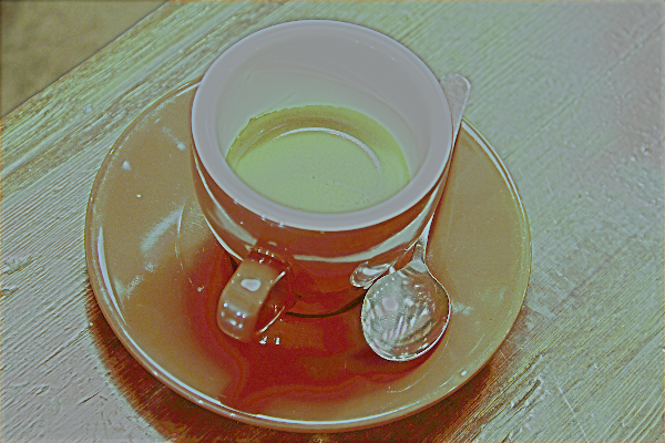
To see these losses at work, the code below trains a tiny Zero-DCE-style network for about half a minute on CPU. It trains on random crops of four skimage images, each darkened by a random factor in linear light, and is tested on the coffee image, which it never sees during training. No ground truth is used. (The loss weights differ from the paper’s because the terms are normalized differently: squared rather than absolute exposure error and mean rather than summed gradients.)

import numpy as np
import torch
import torch.nn as nn
import torch.nn.functional as F
from skimage import data, img_as_float
from skimage.transform import resize

torch.manual_seed(0); rng = np.random.default_rng(0)
darken = lambda x, k: (k * x ** 2.2) ** (1 / 2.2)          # less light, in linear units
train = [resize(img_as_float(f()), (256, 256), anti_aliasing=True)
         for f in (data.astronaut, data.chelsea, data.rocket, data.immunohistochemistry)]

def batch(n=4, size=64):                                  # random crops, random darkness
    xs = []
    for _ in range(n):
        img = train[rng.integers(len(train))]
        i, j = rng.integers(0, 256 - size, 2)
        xs.append(darken(img[i:i + size, j:j + size], rng.uniform(0.02, 0.3)))
    return torch.tensor(np.stack(xs), dtype=torch.float32).permute(0, 3, 1, 2)

class TinyDCE(nn.Module):
    def __init__(self, n_iter=8, w=16):
        super().__init__()
        self.n_iter = n_iter
        self.body = nn.Sequential(
            nn.Conv2d(3, w, 3, padding=1), nn.ReLU(), nn.Conv2d(w, w, 3, padding=1), nn.ReLU(),
            nn.Conv2d(w, w, 3, padding=1), nn.ReLU(), nn.Conv2d(w, 3 * n_iter, 3, padding=1), nn.Tanh())
    def forward(self, x):
        alphas = self.body(x).chunk(self.n_iter, dim=1)    # 8 maps of shape B x 3 x H x W
        y = x
        for a in alphas:
            y = y + a * y * (1 - y)                         # the LE curve
        return y, torch.cat(alphas, 1)

def L_exp(y, E=0.6, p=16):   # mean brightness of 16x16 patches should be near E
    return (F.avg_pool2d(y.mean(1, keepdim=True), p) - E).pow(2).mean()
def L_col(y):                # gray-world: channel means should agree
    r, g, b = y.mean((2, 3)).unbind(1)
    return ((r - g) ** 2 + (r - b) ** 2 + (g - b) ** 2).mean()
def L_tv(a):                 # curve parameters should vary smoothly in space
    return (a[..., 1:, :] - a[..., :-1, :]).pow(2).mean() + (a[..., :, 1:] - a[..., :, :-1]).pow(2).mean()
def L_spa(y, x, p=4):        # keep the contrast between neighbouring 4x4 regions
    Y, X = (F.avg_pool2d(t.mean(1, keepdim=True), p) for t in (y, x))
    return sum(((torch.diff(Y, dim=d) - torch.diff(X, dim=d)) ** 2).mean() for d in (2, 3))

net = TinyDCE()
opt = torch.optim.Adam(net.parameters(), lr=1e-3)
for step in range(600):                                   # ~20-40 s on a laptop CPU
    x = batch()
    y, a = net(x)
    loss = L_spa(y, x) + 10 * L_exp(y) + 5 * L_col(y) + 200 * L_tv(a)
    opt.zero_grad(); loss.backward(); opt.step()

test = darken(img_as_float(data.coffee()), 0.05)          # an image never used in training
with torch.no_grad():
    out, _ = net(torch.tensor(test, dtype=torch.float32).permute(2, 0, 1)[None])
print(f"mean brightness: {test.mean():.3f} -> {out.mean():.3f}")   # about 0.10 -> 0.50

Drag the slider to compare the dark input and the toy’s output:

Dark inputZero-reference toy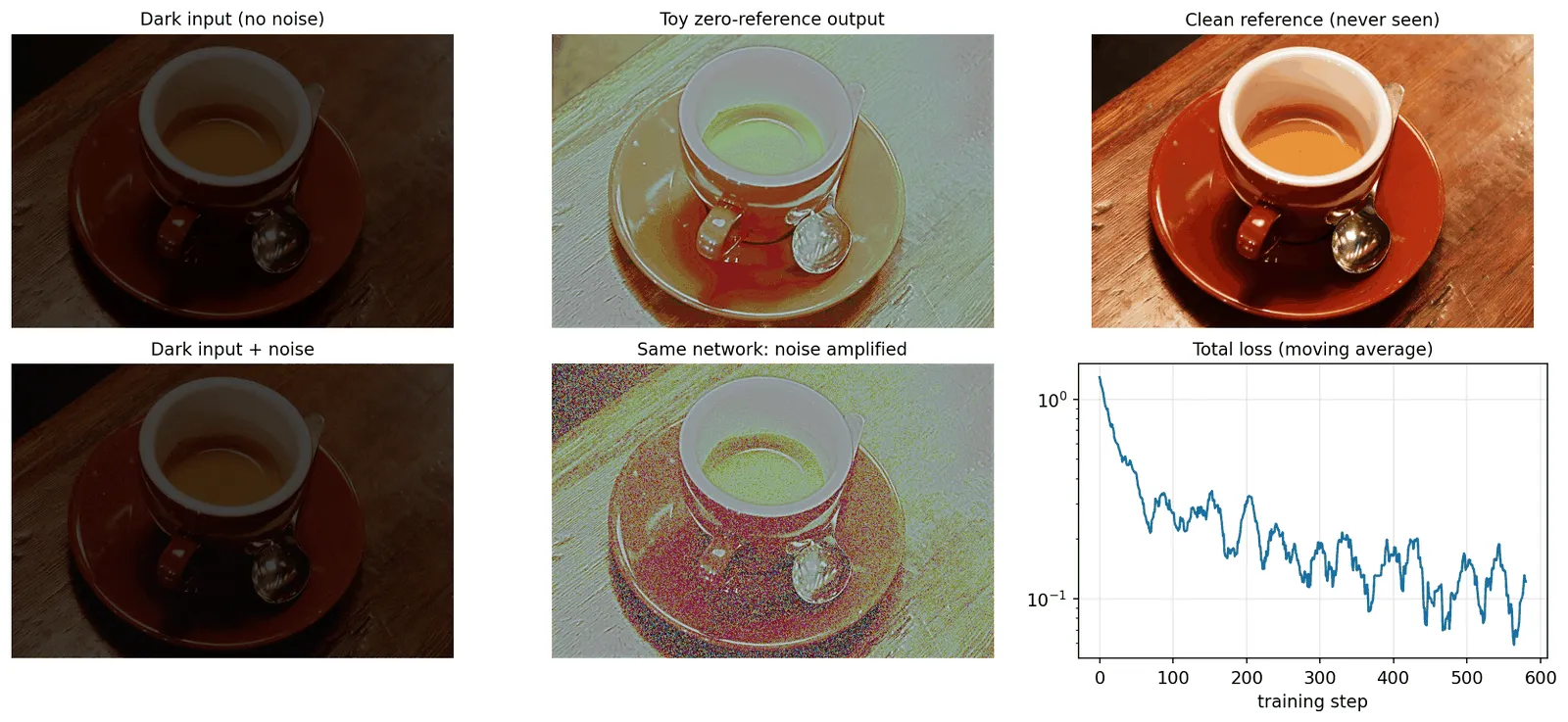

The toy shows the strengths and the limits of the zero-reference idea in one picture. Without a single reference image, the network learns a sensible brightening that transfers to an unseen photo. But each loss is a prior, and priors can be wrong: gray-world fails for scenes that really are red or brown, a fixed exposure target $E$ flattens deliberately dark regions, and nothing in the losses asks for denoising. Real zero-reference methods are trained on many more images, and some add explicit noise handling, but these failure modes are visible in published results too.

Normalizing flows and diffusion models

LLFlow [37] (2022) observes that one dark image has many acceptable bright versions, and a pixel-wise loss averages them into a blurry compromise. It learns a conditional normalizing flow: an invertible network that maps normal-light images to a Gaussian distribution, conditioned on features of the dark input. Those features are guided by priors that echo the classical methods: a histogram-equalized version of the input, a color map (close to the Retinex reflectance) and a noise map.

From 2023, diffusion models entered LLIE. They generate the output by iteratively denoising random noise, conditioned on the dark image, and so can synthesize plausible detail that regression networks blur out:

• Diff-Retinex [38] (2023) first decomposes the image with a Retinex transformer, then uses conditional diffusion models to generate the restored reflectance and illumination.
• GSAD [39] (2023) adds a global structure-aware regularization that uses the image structure to guide a curvature-based constraint on the diffusion trajectory, plus an uncertainty-guided term for hard regions.
• LightenDiffusion [40] (2024) performs Retinex decomposition in a latent space and trains with unpaired data.
• Reti-Diff [41] (2025) runs a latent diffusion model to produce compact Retinex priors that guide a restoration transformer, which reduces the cost of running diffusion at full resolution.

The trade-off is cost and fidelity: many denoising steps make inference slow, and generated details may look right without being true. The survey by Adhikarla et al. [6] organizes this sub-field into six families: intrinsic decomposition, spectral and latent, accelerated, guided, multimodal, and autonomous.

Raw-domain low light

Everything above works on processed sRGB images, where the camera’s pipeline (demosaicking, white balance, denoising, tone curve, compression) has already discarded information. Learning to See in the Dark [44] (2018) instead feeds raw sensor data to a U-Net that replaces the whole pipeline. Its SID dataset has 5,094 short-exposure raw images paired with 424 distinct long-exposure references, from a Sony α7S II (Bayer sensor) and a Fujifilm X-T2 (X-Trans sensor), with exposure ratios of ×100, ×250 and ×300. Raw data keeps the linear relation between photons and values and has more bits, so extreme low light that is hopeless in sRGB becomes recoverable. The cost is that the model is tied to one sensor.

All-in-one restoration

Low-light enhancement is also one task inside general restoration models. InstructIR [43] (2024) takes a natural-language instruction (“make this photo brighter”, “remove the noise”) and restores the image accordingly, covering denoising, deblurring, dehazing and low-light enhancement in one network.

Low light for downstream tasks

If the goal is detection rather than pretty pictures, the usual baseline is “enhance, then detect” (see DL 03 · Object Detection). But enhancement tuned for people is not necessarily what a detector needs. MAET [45] (2021) models the low-light degradation physically and trains the detector to also predict the degradation parameters, so that features become aware of it. FeatEnHancer [46] (2023) enhances hierarchical features inside the network, trained directly with the downstream loss, instead of enhancing pixels.

Evaluation

Plain version. There are two kinds of scores. Full-reference metrics compare the output to a ground-truth photo; no-reference metrics judge the output alone. A third approach asks whether the enhanced image helps a downstream task. Each answers a different question, and each can be gamed.

Full-reference metrics

With a reference $y$ and output $\hat{y}$ (values in $[0, 1]$), PSNR is

$$\mathrm{PSNR} = 10 \log_{10} \frac{1}{\frac{1}{n}\lVert \hat{y} - y \rVert_2^2},$$

where $n$ is the number of values. It is a pure pixel error. SSIM [47] compares local luminance, contrast and structure statistics, which correlates better with perception. LPIPS [48] measures the distance between deep features of the two images; lower is better, and it is sensitive to texture and blur that PSNR ignores.

No-reference metrics

For unpaired test sets (LIME, MEF, NPE, DICM, VV), there is no reference. NIQE [49] fits a multivariate Gaussian to natural-scene statistics of pristine images and reports the distance of the test image’s statistics from it, needing no training on human scores; BRISQUE [50] uses similar features with a regressor trained on human opinion scores. Lower is better for both. They were designed for generic distortions, not for exposure, so they can prefer an over-sharpened or noisy image, and they should be backed by visual comparison or user studies.

The GT-mean pitfall

Plain version. On paired benchmarks, a small difference in overall brightness changes PSNR a lot. Some papers rescale each output so its average brightness matches the ground truth before scoring. That is information you never have in practice.

Precise version. “GT-mean” evaluation scales the output by $\lambda = \mathbb{E}[y]/\mathbb{E}[f(x)]$ and computes the metric on $\lambda f(x)$, where $\mathbb{E}[\cdot]$ is the image mean. Because LLIE is ambiguous about the “right” brightness, this can raise PSNR substantially. The Retinexformer authors provide this mode in their code for comparability with methods such as LLFlow and KinD and recent diffusion models, while explicitly saying they do not recommend it, because it uses the ground truth to correct the output [26]. Liao et al. [51] (2025) study the brightness mismatch between outputs and references and propose a GT-mean loss for training, reporting both standard and GT-mean metrics. When reading tables: check which setting is used, never mix the two, and prefer methods that are good under the standard protocol.

Task-driven evaluation

Since LLIE is often a preprocessing step, another test is to run a detector or segmenter on the enhanced images (on ExDark [57], for example) and report its accuracy. Liu and Fan’s 2025 review [5] finds a disconnect: supervised methods often produce images with high perceptual quality but only modest gains for vision tasks, while zero-shot methods, despite lower image-quality scores, give more consistent gains across tasks. The benchmark of Liu et al. [4] also evaluates face detection in low light. A complete evaluation reports fidelity, no-reference quality, task performance, and runtime.

Benchmark datasets

Plain version. Datasets differ in whether they have pairs, whether the darkness is real or synthetic, whether they are raw or sRGB, and whether they carry labels for detection.

Dataset	Type	Content and what it is for
LOL (v1) [21]	Paired, real, sRGB	500 low/normal pairs captured by changing exposure (485 train / 15 test), 400×600. The most common LLIE benchmark; small test set.
LOL-v2 [52]	Paired, real + synthetic subsets	A larger Real subset of captured pairs and a Synthetic subset of synthesized pairs. Report the two subsets separately.
LSRW [53]	Paired, real	5,650 pairs from a Nikon D7500 (3,170) and a Huawei P40 Pro (2,480); 5,600 train, 50 test. Tests generalization across devices.
SDSD [54]	Paired video	Dynamic indoor and outdoor scenes captured twice with a mechatronic system for alignment; often split into frames for image tests.
SID [44]	Paired, raw	5,094 short-exposure raw images with 424 long-exposure references (Sony and Fuji). Extreme low light, raw-to-sRGB.
MIT-Adobe FiveK [55]	Paired, retouching	5,000 raw photos, each retouched by five experts. Used for tone and color enhancement (photo retouching).
SICE [56]	Multi-exposure sequences	Under- to over-exposed captures of each scene with a reference; used to train exposure correction (e.g. Zero-DCE).
VE-LOL [4]	Paired + detection	VE-LOL-L for enhancement and VE-LOL-H with face annotations for high-level evaluation.
ExDark [57]	Unpaired, labeled	7,363 low-light images, 12 object classes, 10 lighting conditions. Task-driven evaluation (detection).
LIME [17], MEF [58], NPE [18], DICM [59], VV [60]	Unpaired test sets	Small collections of real low-light or non-uniformly lit photos for visual comparison and no-reference metrics.

Challenges: NTIRE 2024 and 2025

The NTIRE workshop at CVPR ran LLIE challenges in consecutive years. The NTIRE 2024 challenge [61] covered ultra-high-resolution (4K and beyond), non-uniform illumination, backlighting, extreme darkness and night scenes; it had 428 registered participants and 22 teams with valid submissions. The NTIRE 2025 challenge [62] had 762 registered participants and 28 teams with valid entries. The reports summarize the winning designs and are a good snapshot of what works under a fixed, fair protocol.

Modern view

The field has moved from hand-made priors to learned models in under a decade, but the core questions in the post [1] are the same: how to model the light, how to handle noise, and how to know whether an output is good. The surveys below are the best entry points.

Li et al., TPAMI 2022 [2]. The most cited deep-LLIE survey. It organizes methods by learning strategy (supervised, reinforcement, unsupervised, zero-shot and semi-supervised learning), network structure, use of the Retinex model, data format (sRGB or raw), loss functions, and training and test data. It also introduces LLIV-Phone, an image and video dataset captured with many different phone cameras under diverse illumination, and an online platform for comparing methods. Its main lessons are a generalization gap (many methods struggle on the phone data) and a frequent mismatch between metric scores and visual quality.

Zheng et al., “Low-Light Image and Video Enhancement: A Comprehensive Survey and Beyond” [3]. It reviews traditional and deep methods with a similar taxonomy and goes further on data: it proposes SICE_Grad and SICE_Mix, which mix under- and over-exposure inside one image, and Night Wenzhou, an aerial and street night video set, to test methods on cases that existing benchmarks miss. It was the source of the post’s own overview figures.

Liu et al., IJCV 2021 [4]. “Benchmarking low-light image enhancement and beyond” is a benchmark more than a survey: the VE-LOL dataset with paired data and face annotations, a comparison using full-reference, no-reference and semantic metrics, and a joint enhancement-plus-detection model. It made task-driven evaluation mainstream.

Liu and Fan, Neurocomputing 2025 [5]. This review asks which enhancement actually helps downstream vision and finds the disconnect described above between image-quality metrics and task performance, with zero-shot methods giving the most consistent task gains.

Adhikarla et al., 2025 [6]. A survey of diffusion models for LLIE with a six-family taxonomy and a performance analysis. Its message is that diffusion brings realism and flexibility but at a high inference cost, so acceleration, guidance and latent-space designs are the active topics.

NTIRE reports [61], [62]. These are not surveys but show the current practice of top teams under a common protocol, with high-resolution and difficult illumination.

State of the art (2023–2026). Three directions dominate. First, Retinex-guided backbones: transformers (Retinexformer [26]) and state-space models (RetinexMamba [42]) that keep a light-versus-reflectance structure. Second, generative models: diffusion (Diff-Retinex [38], GSAD [39], LightenDiffusion [40], Reti-Diff [41]) and flows (LLFlow [37]). Third, better representations and protocols: learned color spaces (HVI-CIDNet [27]), brightness-mismatch-aware training and evaluation (GT-Mean loss [51]), language-guided and all-in-one restoration (CLIP-LIT [36], InstructIR [43]), and task-aware enhancement (MAET [45], FeatEnHancer [46]).

Open problems.

• Real noise. Most sRGB methods train on data whose noise does not match real sensors after a camera pipeline. Better noise models [7], raw-domain training [44], or joint enhancement and denoising remain central.
• Video consistency. Frame-by-frame enhancement flickers. Paired video data (SDSD [54]) is scarce, and temporal consistency is still hard, especially with generative models.
• Evaluation. The ill-posed brightness target, GT-mean protocols, unreliable no-reference metrics for exposure, and the gap between perceptual and task metrics make comparisons fragile.
• Efficiency on edge devices. Phones and cars need real-time, low-power models. Curve methods (Zero-DCE++ [34], SCI [35]) and lightweight prior-based networks [28] show that tiny models can work, while diffusion models remain far too slow for this use.
• Generalization. Models trained on one dataset or camera often fail on another (the generalization gap reported in [2]); mixed over- and under-exposure, backlight and colored artificial light are still difficult.

Key takeaways

• LLIE is tone enhancement plus restoration: a perfect brightness correction still leaves noise, color cast and quantization (Figure 1).
• Brightness can be enhanced in a separate channel ($V$, $I$, $Y'$, $L^*$), but the choice couples to saturation. BT.601 luma is $0.299R' + 0.587G' + 0.114B'$; $16 + 0.257R' + 0.504G' + 0.098B'$ is the same luma in 8-bit limited range.
• Retinex models an image as reflectance times illumination, $S = R \circ L$; SSR/MSR/LIME estimate $L$ with smoothness priors, and the inverted-image dehazing approach rests on essentially the same assumption.
• Deep methods are best organized by training signal: supervised, unrolled, unpaired (EnlightenGAN), zero-reference (Zero-DCE, SCI, CLIP-LIT) and generative (LLFlow, diffusion). Retinex decomposition appears across them.
• Zero-DCE’s LE curve $x + \alpha x(1-x)$ preserves range and order; its non-reference losses are priors (exposure, gray world, smoothness, contrast) that can fail on real noise and colorful scenes.
• Report full-reference, no-reference and task-driven results, never mix GT-mean and standard numbers, and remember that higher PSNR does not guarantee better detection.

Exercises

1. Monotonic curves. Show that $\mathrm{LE}(x;\alpha) = x + \alpha x(1-x)$ is monotonically non-decreasing on $[0, 1]$ if and only if $|\alpha| \le 1$. What goes wrong for $\alpha = 1.5$?

Hint

The derivative is $1 + \alpha(1 - 2x)$, which is linear in $x$, so its minimum on $[0, 1]$ is at an endpoint: $1 + \alpha$ at $x = 0$ or $1 - \alpha$ at $x = 1$. Both are $\ge 0$ exactly when $|\alpha| \le 1$. For $\alpha = 1.5$ the slope at $x = 1$ is $-0.5$, so near-white pixels would get darker as the input gets brighter, reversing the brightness order and creating artifacts in highlights.

2. Gain of the iterated curve. For a small input $x$, show that eight iterations with a constant $\alpha$ multiply $x$ by approximately $(1 + \alpha)^8$. Use this to explain why zero-reference curve methods amplify shadow noise, and suggest one change to the losses or architecture that would reduce the problem.

Hint

For small $x$, $x(1 - x) \approx x$, so each step gives $x \mapsto (1 + \alpha)x$. With $\alpha = 1$ that is $2^8 = 256$. Noise with standard deviation $\sigma$ becomes $256\sigma$. Possible fixes: add a denoising branch or a noise-aware loss, limit $\alpha$ where the estimated SNR is low (in the spirit of SNR-aware), or penalize high-frequency energy in the output that is not present in a smoothed input.

3. Two luma formulas. A pixel has $(R', G', B') = (200, 100, 50)$ in 8 bits. Compute its full-range BT.601 luma and its limited-range luma. Show that they encode the same quantity.

Hint

Full range: $0.299 \cdot 200 + 0.587 \cdot 100 + 0.114 \cdot 50 = 124.2$. Limited range: $16 + 0.257 \cdot 200 + 0.504 \cdot 100 + 0.098 \cdot 50 \approx 122.7$. Converting back: $(122.7 - 16) \cdot 255/219 \approx 124.2$. The only differences are the scale $219/255$ and the offset 16.

4. Retinex losses without ground truth. In Retinex-Net, why is $\mathcal{L}_{ir} = \lVert R_{\text{low}} - R_{\text{normal}}\rVert_1$ needed? Describe a trivial decomposition that zeroes the self-reconstruction terms of $\mathcal{L}_{\text{recon}}$ and $\mathcal{L}_{is}$ but is useless, and explain how $\mathcal{L}_{ir}$ rules it out.

Hint

Set $I_i \equiv 1$ (perfectly smooth) and $R_i = S_i$. Then each image is reconstructed exactly and the smoothness loss is zero, but nothing has been decomposed. Since $S_{\text{low}} \neq S_{\text{normal}}$, this gives $R_{\text{low}} \neq R_{\text{normal}}$, so $\mathcal{L}_{ir}$ is large. Requiring equal reflectances forces the brightness difference between the pair into the illumination.

5. GT-mean by hand. Your model outputs an image with mean 0.40; the ground truth has mean 0.50, and otherwise the output is perfect up to that global scale. What is the GT-mean scale factor, and what is the PSNR before and after rescaling if the image is a constant? Why is the rescaled number not a fair comparison with a method evaluated normally?

Hint

$\lambda = 0.50/0.40 = 1.25$. Before: MSE $= 0.1^2 = 0.01$, PSNR $= 20$ dB. After rescaling the output equals the reference, so the error is 0 and PSNR is unbounded. A real method never has the ground-truth mean at test time, so GT-mean numbers reward the right structure while ignoring the hardest part of the task, choosing the brightness.

6. Change the color prior. In the PyTorch toy, replace the gray-world loss with a loss that keeps the chromaticity of the input, for example $\lVert y / \sum_c y_c - x / \sum_c x_c \rVert_1$. Train again and compare the coffee result with Figure 7. When is each prior preferable?

Hint

Add a small epsilon to the sums. Preserving input chromaticity keeps the red-brown cup red, but it also keeps any color cast of the light source (for example a sodium lamp). Gray world removes casts but desaturates scenes that are genuinely colorful. Real methods often combine a weak color prior with learned color correction from data.

References

1. Shyandram, “簡介Deep Learning Low-Light Image Enhancement (LLIE)” (Introduction to deep-learning low-light image enhancement, in Chinese), blog post, 2024; updated 2026. link
2. C. Li, C. Guo, L. Han, J. Jiang, M.-M. Cheng, J. Gu and C. C. Loy, “Low-light image and video enhancement using deep learning: A survey,” IEEE Transactions on Pattern Analysis and Machine Intelligence, vol. 44, no. 12, pp. 9396–9416, 2022. arXiv
3. S. Zheng, Y. Ma, J. Pan, C. Lu and G. Gupta, “Low-light image and video enhancement: A comprehensive survey and beyond,” arXiv:2212.10772, 2022. arXiv
4. J. Liu, D. Xu, W. Yang, M. Fan and H. Huang, “Benchmarking low-light image enhancement and beyond,” International Journal of Computer Vision, vol. 129, no. 4, pp. 1153–1184, 2021. doi project
5. F. Liu and L. Fan, “A review of advancements in low-light image enhancement using deep learning,” Neurocomputing, vol. 652, art. 131052, 2025. arXiv
6. E. Adhikarla, Y. Liu and B. D. Davison, “Diffusion models for low-light image enhancement: A multi-perspective taxonomy and performance analysis,” arXiv:2510.05976, 2025. arXiv
7. A. Foi, M. Trimeche, V. Katkovnik and K. Egiazarian, “Practical Poissonian-Gaussian noise modeling and fitting for single-image raw-data,” IEEE Transactions on Image Processing, vol. 17, no. 10, pp. 1737–1754, 2008. doi
8. ITU-R, “Recommendation BT.601-7: Studio encoding parameters of digital television for standard 4:3 and wide-screen 16:9 aspect ratios,” 2011. ITU
9. S. M. Pizer, E. P. Amburn, J. D. Austin, et al., “Adaptive histogram equalization and its variations,” Computer Vision, Graphics, and Image Processing, vol. 39, no. 3, pp. 355–368, 1987. doi
10. K. Zuiderveld, “Contrast limited adaptive histogram equalization,” in Graphics Gems IV, Academic Press, 1994, pp. 474–485. doi
11. E. H. Land, “The retinex theory of color vision,” Scientific American, vol. 237, no. 6, pp. 108–128, 1977. doi
12. D. J. Jobson, Z. Rahman and G. A. Woodell, “Properties and performance of a center/surround retinex,” IEEE Transactions on Image Processing, vol. 6, pp. 451–462, 1997. doi
13. D. J. Jobson, Z. Rahman and G. A. Woodell, “A multiscale retinex for bridging the gap between color images and the human observation of scenes,” IEEE Transactions on Image Processing, vol. 6, no. 7, pp. 965–976, 1997. doi
14. K. He, J. Sun and X. Tang, “Single image haze removal using dark channel prior,” IEEE Transactions on Pattern Analysis and Machine Intelligence, vol. 33, no. 12, pp. 2341–2353, 2011. doi
15. X. Dong, Y. Pang and J. Wen, “Fast efficient algorithm for enhancement of low lighting video,” ACM SIGGRAPH 2010 Posters, 2010. SIGGRAPH history doi
16. X. Dong, G. Wang, Y. Pang, W. Li, J. Wen, W. Meng and Y. Lu, “Fast efficient algorithm for enhancement of low lighting video,” in Proc. IEEE International Conference on Multimedia and Expo (ICME), 2011. doi
17. X. Guo, Y. Li and H. Ling, “LIME: Low-light image enhancement via illumination map estimation,” IEEE Transactions on Image Processing, vol. 26, no. 2, pp. 982–993, 2017. doi
18. S. Wang, J. Zheng, H.-M. Hu and B. Li, “Naturalness preserved enhancement algorithm for non-uniform illumination images,” IEEE Transactions on Image Processing, vol. 22, no. 9, pp. 3538–3548, 2013. doi
19. K. G. Lore, A. Akintayo and S. Sarkar, “LLNet: A deep autoencoder approach to natural low-light image enhancement,” Pattern Recognition, vol. 61, pp. 650–662, 2017. doi
20. L. Tao, C. Zhu, J. Song, T. Lu, H. Jia and X. Xie, “Low-light image enhancement using CNN and bright channel prior,” in Proc. IEEE International Conference on Image Processing (ICIP), 2017, pp. 3215–3219. doi
21. C. Wei, W. Wang, W. Yang and J. Liu, “Deep retinex decomposition for low-light enhancement,” in Proc. British Machine Vision Conference (BMVC), 2018. arXiv project
22. Y. Zhang, J. Zhang and X. Guo, “Kindling the darkness: A practical low-light image enhancer,” in Proc. ACM International Conference on Multimedia (ACM MM), 2019, pp. 1632–1640. doi
23. Y. Zhang, X. Guo, J. Ma, W. Liu and J. Zhang, “Beyond brightening low-light images,” International Journal of Computer Vision, vol. 129, no. 4, pp. 1013–1037, 2021. doi
24. S. W. Zamir, A. Arora, S. Khan, et al., “Learning enriched features for real image restoration and enhancement,” in Proc. European Conference on Computer Vision (ECCV), 2020, pp. 492–511. arXiv
25. X. Xu, R. Wang, C.-W. Fu and J. Jia, “SNR-aware low-light image enhancement,” in Proc. IEEE/CVF CVPR, 2022, pp. 17693–17703. doi
26. Y. Cai, H. Bian, J. Lin, H. Wang, R. Timofte and Y. Zhang, “Retinexformer: One-stage Retinex-based transformer for low-light image enhancement,” in Proc. IEEE/CVF ICCV, 2023. arXiv code
27. Q. Yan, Y. Feng, C. Zhang, et al., “HVI: A new color space for low-light image enhancement,” in Proc. IEEE/CVF CVPR, 2025. arXiv
28. S.-E. Weng, S.-G. Miaou and R. Christanto, “A lightweight low-light image enhancement network via channel prior and gamma correction,” International Journal of Pattern Recognition and Artificial Intelligence, vol. 39, no. 12, art. 2554013, 2025. doi code
29. S.-E. Weng, C.-Y. Hsiao, L.-W. Lu, et al., “Rethinking theoretical illumination for efficient low-light image enhancement” (CPGA-Net+), arXiv:2409.05274, 2024. arXiv
30. R. Liu, L. Ma, J. Zhang, X. Fan and Z. Luo, “Retinex-inspired unrolling with cooperative prior architecture search for low-light image enhancement,” in Proc. IEEE/CVF CVPR, 2021, pp. 10556–10565. arXiv
31. W. Wu, J. Weng, P. Zhang, X. Wang, W. Yang and J. Jiang, “URetinex-Net: Retinex-based deep unfolding network for low-light image enhancement,” in Proc. IEEE/CVF CVPR, 2022, pp. 5891–5900. doi
32. Y. Jiang, X. Gong, D. Liu, et al., “EnlightenGAN: Deep light enhancement without paired supervision,” IEEE Transactions on Image Processing, vol. 30, pp. 2340–2349, 2021. arXiv
33. C. Guo, C. Li, J. Guo, et al., “Zero-reference deep curve estimation for low-light image enhancement,” in Proc. IEEE/CVF CVPR, 2020, pp. 1777–1786. arXiv
34. C. Li, C. Guo and C. C. Loy, “Learning to enhance low-light image via zero-reference deep curve estimation,” IEEE Transactions on Pattern Analysis and Machine Intelligence, vol. 44, no. 8, 2022. arXiv
35. L. Ma, T. Ma, R. Liu, X. Fan and Z. Luo, “Toward fast, flexible, and robust low-light image enhancement,” in Proc. IEEE/CVF CVPR, 2022, pp. 5627–5636. arXiv
36. Z. Liang, C. Li, S. Zhou, R. Feng and C. C. Loy, “Iterative prompt learning for unsupervised backlit image enhancement,” in Proc. IEEE/CVF ICCV, 2023. arXiv
37. Y. Wang, R. Wan, W. Yang, H. Li, L.-P. Chau and A. C. Kot, “Low-light image enhancement with normalizing flow,” in Proc. AAAI Conference on Artificial Intelligence, vol. 36, no. 3, pp. 2604–2612, 2022. arXiv
38. X. Yi, H. Xu, H. Zhang, L. Tang and J. Ma, “Diff-Retinex: Rethinking low-light image enhancement with a generative diffusion model,” in Proc. IEEE/CVF ICCV, 2023. arXiv
39. J. Hou, Z. Zhu, J. Hou, H. Liu, H. Zeng and H. Yuan, “Global structure-aware diffusion process for low-light image enhancement,” in Advances in Neural Information Processing Systems (NeurIPS), 2023. arXiv
40. H. Jiang, A. Luo, X. Liu, S. Han and S. Liu, “LightenDiffusion: Unsupervised low-light image enhancement with latent-Retinex diffusion models,” in Proc. European Conference on Computer Vision (ECCV), 2024. arXiv
41. C. He, C. Fang, Y. Zhang, et al., “Reti-Diff: Illumination degradation image restoration with Retinex-based latent diffusion model,” in Proc. International Conference on Learning Representations (ICLR), 2025. proceedings
42. J. Bai, Y. Yin, Q. He, Y. Li and X. Zhang, “RetinexMamba: Retinex-based Mamba for low-light image enhancement,” arXiv:2405.03349, 2024. arXiv
43. M. V. Conde, G. Geigle and R. Timofte, “InstructIR: High-quality image restoration following human instructions,” in Proc. European Conference on Computer Vision (ECCV), 2024. arXiv
44. C. Chen, Q. Chen, J. Xu and V. Koltun, “Learning to see in the dark,” in Proc. IEEE/CVF CVPR, 2018, pp. 3291–3300. arXiv
45. Z. Cui, G.-J. Qi, L. Gu, S. You, Z. Zhang and T. Harada, “Multitask AET with orthogonal tangent regularity for dark object detection,” in Proc. IEEE/CVF ICCV, 2021. arXiv
46. K. A. Hashmi, G. Kallempudi, D. Stricker and M. Z. Afzal, “FeatEnHancer: Enhancing hierarchical features for object detection and beyond under low-light vision,” in Proc. IEEE/CVF ICCV, 2023. arXiv
47. Z. Wang, A. C. Bovik, H. R. Sheikh and E. P. Simoncelli, “Image quality assessment: From error visibility to structural similarity,” IEEE Transactions on Image Processing, vol. 13, no. 4, pp. 600–612, 2004. doi
48. R. Zhang, P. Isola, A. A. Efros, E. Shechtman and O. Wang, “The unreasonable effectiveness of deep features as a perceptual metric,” in Proc. IEEE/CVF CVPR, 2018. arXiv
49. A. Mittal, R. Soundararajan and A. C. Bovik, “Making a ‘completely blind’ image quality analyzer,” IEEE Signal Processing Letters, vol. 20, no. 3, pp. 209–212, 2013. doi
50. A. Mittal, A. K. Moorthy and A. C. Bovik, “No-reference image quality assessment in the spatial domain,” IEEE Transactions on Image Processing, vol. 21, no. 12, pp. 4695–4708, 2012. doi
51. J. Liao, S. Hao, R. Hong and M. Wang, “GT-Mean loss: A simple yet effective solution for brightness mismatch in low-light image enhancement,” in Proc. IEEE/CVF ICCV, 2025. arXiv
52. W. Yang, W. Wang, H. Huang, S. Wang and J. Liu, “Sparse gradient regularized deep Retinex network for robust low-light image enhancement,” IEEE Transactions on Image Processing, vol. 30, pp. 2072–2086, 2021. doi
53. J. Hai, Z. Xuan, R. Yang, et al., “R2RNet: Low-light image enhancement via Real-low to Real-normal Network,” Journal of Visual Communication and Image Representation, vol. 90, art. 103712, 2023. arXiv
54. R. Wang, X. Xu, C.-W. Fu, et al., “Seeing dynamic scene in the dark: A high-quality video dataset with mechatronic alignment,” in Proc. IEEE/CVF ICCV, 2021, pp. 9680–9689. doi code
55. V. Bychkovsky, S. Paris, E. Chan and F. Durand, “Learning photographic global tonal adjustment with a database of input/output image pairs,” in Proc. IEEE CVPR, 2011, pp. 97–104. dataset
56. J. Cai, S. Gu and L. Zhang, “Learning a deep single image contrast enhancer from multi-exposure images,” IEEE Transactions on Image Processing, vol. 27, no. 4, pp. 2049–2062, 2018. doi
57. Y. P. Loh and C. S. Chan, “Getting to know low-light images with the Exclusively Dark dataset,” Computer Vision and Image Understanding, vol. 178, pp. 30–42, 2019. arXiv
58. K. Ma, K. Zeng and Z. Wang, “Perceptual quality assessment for multi-exposure image fusion,” IEEE Transactions on Image Processing, vol. 24, no. 11, pp. 3345–3356, 2015. doi
59. C. Lee, C. Lee and C.-S. Kim, “Contrast enhancement based on layered difference representation of 2D histograms,” IEEE Transactions on Image Processing, vol. 22, no. 12, pp. 5372–5384, 2013. doi
60. V. Vonikakis, “Datasets” (source of the VV test images), personal web page. link
61. X. Liu, Z. Wu, A. Li, et al., “NTIRE 2024 challenge on low light image enhancement: Methods and results,” in Proc. IEEE/CVF CVPR Workshops, 2024. arXiv
62. X. Liu, Z. Wu, F.-A. Vasluianu, et al., “NTIRE 2025 challenge on low light image enhancement: Methods and results,” in Proc. IEEE/CVF CVPR Workshops, 2025. arXiv