DL 03 · Object Detection: From R-CNN to DETR

What you’ll learn

• What a detector outputs (boxes, class labels, confidences), and how detection differs from classification, semantic segmentation and instance segmentation.
• The building blocks every modern detector shares, in math and in code: box parameterization and regression targets, IoU and its GIoU/DIoU/CIoU variants, anchors and label assignment, non-maximum suppression, feature pyramids and the focal loss.
• How the four big families work and why each was invented: two-stage (R-CNN to Cascade R-CNN), one-stage (YOLO, SSD, RetinaNet), anchor-free (CornerNet, CenterNet, FCOS) and set prediction with transformers (DETR to RT-DETR).
• How open-vocabulary and grounding detectors (OWL-ViT, Grounding DINO, YOLO-World) and promptable foundation models change what “the class list” means.
• How detection is evaluated (precision–recall, AP, VOC and COCO protocols, AP50/AP75/APs/m/l), which datasets matter, and what limits speed in deployment.

The big picture

A classifier answers one question about a whole image: what is this? A detector answers a harder one: what is where? It must find every object of interest, draw a tight rectangle (a bounding box) around each, name it, and say how sure it is. The number of objects is not known in advance: there may be zero, one or three hundred.

Detection is the entry point of most “real” vision systems. Self-driving cars detect pedestrians and vehicles; phones detect faces before focusing; factories detect defects; trackers (see the tracking chapter linked at the end) mostly link detections over time. The field also produced many ideas that now appear everywhere in deep learning: multi-task losses, feature pyramids, the focal loss, and set prediction with bipartite matching.

This tutorial assumes you know CNNs and image classification (DL 02) and the classical feature ideas of DIP Chapter 12. Two surveys frame the whole story: Zou et al., Object Detection in 20 Years [1], and Liu et al.’s IJCV survey of deep generic detection [2]. We return to both in the Modern view.

The detection problem

Plain version. The input is an image. The output is a short list of (box, class, score) triples. The training data is a list of human-drawn boxes with class names.

Precise version. Given an image $I \in \mathbb{R}^{H \times W \times 3}$, a detector outputs a set

$$\hat{Y} = \{(\hat{b}_i, \hat{c}_i, \hat{s}_i)\}_{i=1}^{N},$$

where $\hat{b}_i \in \mathbb{R}^4$ is a box, $\hat{c}_i \in \{1, \dots, K\}$ is one of $K$ classes, $\hat{s}_i \in [0, 1]$ is a confidence score, and $N$ varies from image to image. The ground truth is a set $Y = \{(b_j, c_j)\}_{j=1}^{M}$ of $M$ annotated objects. Two box formats are common: corners $(x_1, y_1, x_2, y_2)$ and center–size $(c_x, c_y, w, h)$. Boxes are axis-aligned; rotated boxes are a separate variant used for aerial images and text.

Three properties make detection harder than classification:

1. Variable-size output. The network must decide how many things to output. Every architecture in this tutorial is, at heart, a different answer to this problem.
2. Localization and recognition at once. The model must be invariant to what changes about an object’s appearance but sensitive to where it is, a tension that shapes the design of every head.
3. Extreme imbalance. A typical image has a handful of objects but tens of thousands of candidate positions and sizes, nearly all background.

Detection versus its neighbours

Figure 1 compares the four classic recognition tasks on one synthetic scene. Classification gives one label per image. Detection gives a box and a label per object. Semantic segmentation labels every pixel with a class, so two touching balls merge into one blob. Instance segmentation gives each object its own pixel mask, which is detection plus a mask per box; Mask R-CNN [16] is the standard way to get it, as we will see.

Classical detection: sliding windows and hand-made features

Plain version. Before deep learning, detection was “classification in a loop”: cut out a window at every position and size, ask a classifier whether it contains the object, and keep the windows that say yes.

Sliding windows. For a window of fixed size $w \times h$ slid with stride $s$ over an image pyramid with scale factor $\lambda$, the number of windows is roughly

$$N_{\text{win}} \approx \sum_{k \ge 0} \frac{(H \lambda^{-k} - h)(W \lambda^{-k} - w)}{s^2},$$

where $k$ indexes the pyramid levels. For a $640 \times 480$ image, a $64 \times 128$ window, $s = 8$ and $\lambda = 1.2$, that is on the order of $10^4$ windows for one aspect ratio, all of which must be classified. This is the template matching of DIP Chapter 13 scaled up, and it has the same weaknesses: one template shape, many scales, and a lot of wasted work on background.

Viola–Jones (2001) [5] made real-time face detection possible with three tricks. Haar-like features (differences of sums over adjacent rectangles) can be evaluated in constant time using an integral image $S(x, y) = \sum_{x' \le x, y' \le y} I(x', y')$, so any rectangle sum needs four lookups. AdaBoost selects a small set of informative features out of a huge pool. An attentional cascade of increasingly complex classifiers rejects most background windows after only a few feature evaluations, which is the first big idea for beating the imbalance problem: spend computation only where it might matter.

HOG + linear SVM (2005) [6] replaced raw intensities with histograms of oriented gradients, close relatives of the gradient-orientation descriptors in DIP Chapter 12. The detection window is divided into small cells; each cell stores a histogram of gradient orientations weighted by magnitude; overlapping blocks of cells are contrast-normalized; the concatenated vector is scored by a linear SVM. HOG is robust to small shifts and illumination changes, and it made pedestrian detection practical.

Deformable part models (DPM) [7] added structure. An object is a coarse root HOG filter plus several higher-resolution part filters that may shift relative to the root, paying a quadratic deformation cost:

$$\text{score}(p_0) = F_0 \cdot \phi(p_0) + \sum_{i=1}^{n} \max_{p_i} \Big[ F_i \cdot \phi(p_i) - d_i \cdot \psi(p_i - p_0) \Big] + \beta,$$

where $p_0$ is the root position, $p_i$ the position of part $i$, $F_i$ the learned filters, $\phi(\cdot)$ the HOG features at a position, $\psi$ the displacement features $(dx, dy, dx^2, dy^2)$, $d_i$ learned deformation weights and $\beta$ a bias. Part positions are latent variables, trained with a latent SVM. DPM and its variants dominated the PASCAL VOC benchmark [3] until 2012.

Why this era ended. Classical detectors were slow (an exhaustive scan over positions, scales and aspect ratios, each scored by a hand-designed pipeline) and brittle (one hand-designed feature type, a few rigid templates, and poor transfer to new categories, viewpoints and clutter). They also had no way to share features across classes. Deep detectors kept the useful ideas, such as scanning in a feature pyramid, cascades, parts and hard-negative mining, and replaced the hand-made features with learned ones.

Core building blocks

Every detector in the rest of this tutorial is assembled from the same parts. We define each one carefully, with code you can run.

Box parameterization and regression targets

Plain version. A network is bad at outputting absolute pixel coordinates, but good at outputting small corrections. So we start from a reference box (a proposal, an anchor or a point) and predict how to nudge it.

Given a reference box $P = (P_x, P_y, P_w, P_h)$ in center–size form and its matched ground-truth box $G = (G_x, G_y, G_w, G_h)$, the standard targets introduced with R-CNN [8] are

$$t_x = \frac{G_x - P_x}{P_w}, \qquad t_y = \frac{G_y - P_y}{P_h}, \qquad t_w = \log\frac{G_w}{P_w}, \qquad t_h = \log\frac{G_h}{P_h}.$$

Dividing the shift by the reference size makes the target scale-invariant (a 10-pixel error matters more for a 20-pixel box than for a 400-pixel box). The log for width and height makes scaling symmetric (doubling and halving are $+\log 2$ and $-\log 2$) and keeps the decoded size positive: $\hat{G}_w = P_w \exp(\hat{t}_w)$. In practice the targets are often divided by fixed standard deviations, such as $(0.1, 0.1, 0.2, 0.2)$, so that all four have similar magnitude.

import numpy as np

def to_cxcywh(b):
    return np.stack([(b[:, 0] + b[:, 2]) / 2, (b[:, 1] + b[:, 3]) / 2,
                     b[:, 2] - b[:, 0], b[:, 3] - b[:, 1]], axis=1)

def to_xyxy(c):
    return np.stack([c[:, 0] - c[:, 2] / 2, c[:, 1] - c[:, 3] / 2,
                     c[:, 0] + c[:, 2] / 2, c[:, 1] + c[:, 3] / 2], axis=1)

def encode(anchors, gt, std=(0.1, 0.1, 0.2, 0.2)):
    """Regression targets (tx, ty, tw, th) of gt relative to anchors (both xyxy)."""
    P, G = to_cxcywh(anchors), to_cxcywh(gt)
    t = np.stack([(G[:, 0] - P[:, 0]) / P[:, 2],
                  (G[:, 1] - P[:, 1]) / P[:, 3],
                  np.log(G[:, 2] / P[:, 2]),
                  np.log(G[:, 3] / P[:, 3])], axis=1)
    return t / np.array(std)          # normalize so all four have similar scale

def decode(anchors, t, std=(0.1, 0.1, 0.2, 0.2)):
    P = to_cxcywh(anchors)
    t = t * np.array(std)
    c = np.stack([P[:, 0] + t[:, 0] * P[:, 2],
                  P[:, 1] + t[:, 1] * P[:, 3],
                  P[:, 2] * np.exp(t[:, 2]),
                  P[:, 3] * np.exp(t[:, 3])], axis=1)
    return to_xyxy(c)

anchors = np.array([[0, 0, 32, 32], [100, 100, 228, 164]], float)
gt      = np.array([[4, 2, 40, 30], [90, 110, 250, 170]], float)
t = encode(anchors, gt)
print(np.round(t, 3))
print(np.allclose(decode(anchors, t), gt))   # round trip

[[ 1.875  0.     0.589 -0.668]
 [ 0.469  1.25   1.116 -0.323]]
True

These targets are usually trained with the smooth L1 (Huber) loss of Fast R-CNN [9],

$$\text{smooth}_{L_1}(x) = \begin{cases} 0.5\,x^2 & \text{if } |x| \lt 1, \\ |x| - 0.5 & \text{otherwise}, \end{cases}$$

applied to each coordinate difference $x = \hat{t} - t$. It behaves like L2 for small errors (smooth gradients) and like L1 for large ones (robust to outliers early in training). Its weakness is that the four coordinates are treated as independent numbers, while the evaluation metric, IoU, treats the box as a whole. That mismatch motivated IoU-based losses.

IoU and its variants

Plain version. IoU asks: of all the area covered by either box, what fraction is covered by both? It is 1 for a perfect match and 0 for boxes that do not touch.

For two boxes $A$ and $B$,

$$\text{IoU}(A, B) = \frac{|A \cap B|}{|A \cup B|} = \frac{|A \cap B|}{|A| + |B| - |A \cap B|},$$

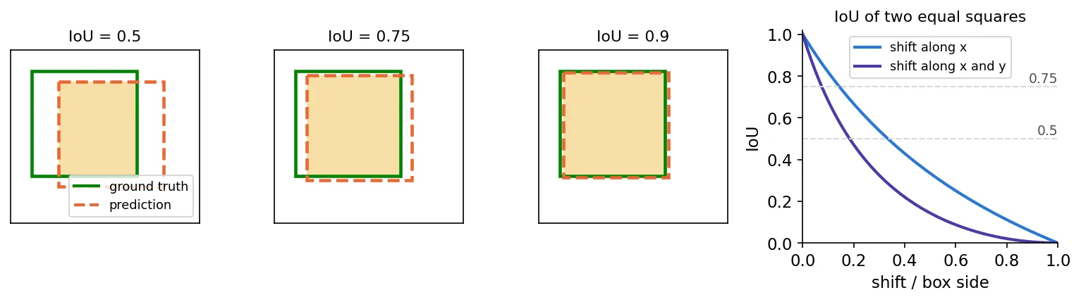
where $|\cdot|$ is area. IoU is scale-invariant, and it is the yardstick for evaluation (a detection counts as correct if its IoU with an unmatched ground-truth box exceeds a threshold), for label assignment and for NMS. Figure 2 shows how demanding the thresholds are: shifting a square by only about 18% of its side along both axes already drops IoU to 0.5.

As a loss, $1 - \text{IoU}$ has a flaw: when two boxes do not overlap, IoU is 0 no matter how far apart they are, so the gradient is zero. Three fixes are widely used:

• GIoU [11] adds a penalty based on the smallest box $C$ that encloses both: $\text{GIoU} = \text{IoU} - \dfrac{|C \setminus (A \cup B)|}{|C|}$, which lies in $(-1, 1]$ and keeps decreasing as non-overlapping boxes drift apart.
• DIoU [12] penalizes the distance between centers directly: $\text{DIoU} = \text{IoU} - \dfrac{\rho^2(\mathbf{b}, \mathbf{b}^{gt})}{c^2}$, where $\rho$ is the Euclidean distance between the box centers $\mathbf{b}$ and $\mathbf{b}^{gt}$, and $c$ is the diagonal length of $C$. It converges faster than GIoU because it pulls the centers together even when one box contains the other, where the GIoU penalty vanishes.
• CIoU [12] adds an aspect-ratio term: $\text{CIoU} = \text{DIoU} - \alpha v$, with $v = \frac{4}{\pi^2}\big(\arctan\frac{w^{gt}}{h^{gt}} - \arctan\frac{w}{h}\big)^2$ measuring aspect-ratio mismatch and $\alpha = \frac{v}{(1 - \text{IoU}) + v}$ a trade-off weight.

The corresponding losses are $1 - \text{GIoU}$, $1 - \text{DIoU}$ and $1 - \text{CIoU}$.

import numpy as np

def iou_family(a, b, eps=1e-9):
    """a, b: (N, 4) boxes as (x1, y1, x2, y2). Returns IoU, GIoU, DIoU, CIoU."""
    ix1, iy1 = np.maximum(a[:, 0], b[:, 0]), np.maximum(a[:, 1], b[:, 1])
    ix2, iy2 = np.minimum(a[:, 2], b[:, 2]), np.minimum(a[:, 3], b[:, 3])
    inter = np.clip(ix2 - ix1, 0, None) * np.clip(iy2 - iy1, 0, None)
    wa, ha = a[:, 2] - a[:, 0], a[:, 3] - a[:, 1]
    wb, hb = b[:, 2] - b[:, 0], b[:, 3] - b[:, 1]
    union = wa * ha + wb * hb - inter
    iou = inter / (union + eps)
    # smallest enclosing box C
    cx1, cy1 = np.minimum(a[:, 0], b[:, 0]), np.minimum(a[:, 1], b[:, 1])
    cx2, cy2 = np.maximum(a[:, 2], b[:, 2]), np.maximum(a[:, 3], b[:, 3])
    area_c = (cx2 - cx1) * (cy2 - cy1)
    giou = iou - (area_c - union) / (area_c + eps)
    # center distance over enclosing-box diagonal
    rho2 = ((a[:, 0] + a[:, 2]) - (b[:, 0] + b[:, 2])) ** 2 / 4 \
         + ((a[:, 1] + a[:, 3]) - (b[:, 1] + b[:, 3])) ** 2 / 4
    c2 = (cx2 - cx1) ** 2 + (cy2 - cy1) ** 2
    diou = iou - rho2 / (c2 + eps)
    v = 4 / np.pi**2 * (np.arctan(wb / hb) - np.arctan(wa / ha)) ** 2
    alpha = v / (1 - iou + v + eps)
    ciou = diou - alpha * v
    return iou, giou, diou, ciou

gt = np.array([[10, 10, 50, 50]] * 3, float)
pred = np.array([[20, 20, 60, 60],    # overlapping, shifted
                 [60, 10, 100, 50],   # disjoint, nearby
                 [200, 10, 240, 50]], float)  # disjoint, far away
for name, v in zip(["IoU", "GIoU", "DIoU", "CIoU"], iou_family(pred, gt)):
    print(f"{name:5s}", np.round(v, 3))

IoU   [0.391 0.    0.   ]
GIoU  [ 0.311 -0.111 -0.652]
DIoU  [ 0.351 -0.258 -0.662]
CIoU  [ 0.351 -0.258 -0.662]

The two disjoint predictions both have IoU 0, but GIoU and DIoU correctly say that the far one is worse. CIoU equals DIoU here because all boxes are squares, so there is no aspect-ratio mismatch.

Anchors and label assignment

Plain version. Instead of searching freely, a dense detector places a fixed set of reference boxes, anchors, at every cell of a feature map, and each anchor asks: “is there an object roughly like me here, and how should I move to fit it?”

At a feature map with stride $s$ (each cell covers $s \times s$ input pixels), anchors are centered at $\big((i + \tfrac12) s, (j + \tfrac12) s\big)$ with a few scales $\sigma$ and aspect ratios $r = h/w$, giving widths $w = \sigma/\sqrt{r}$ and heights $h = \sigma\sqrt{r}$ so that the area stays $\sigma^2$. Faster R-CNN uses 3 scales $\times$ 3 ratios $= 9$ anchors per location [10] (Figure 3, left).

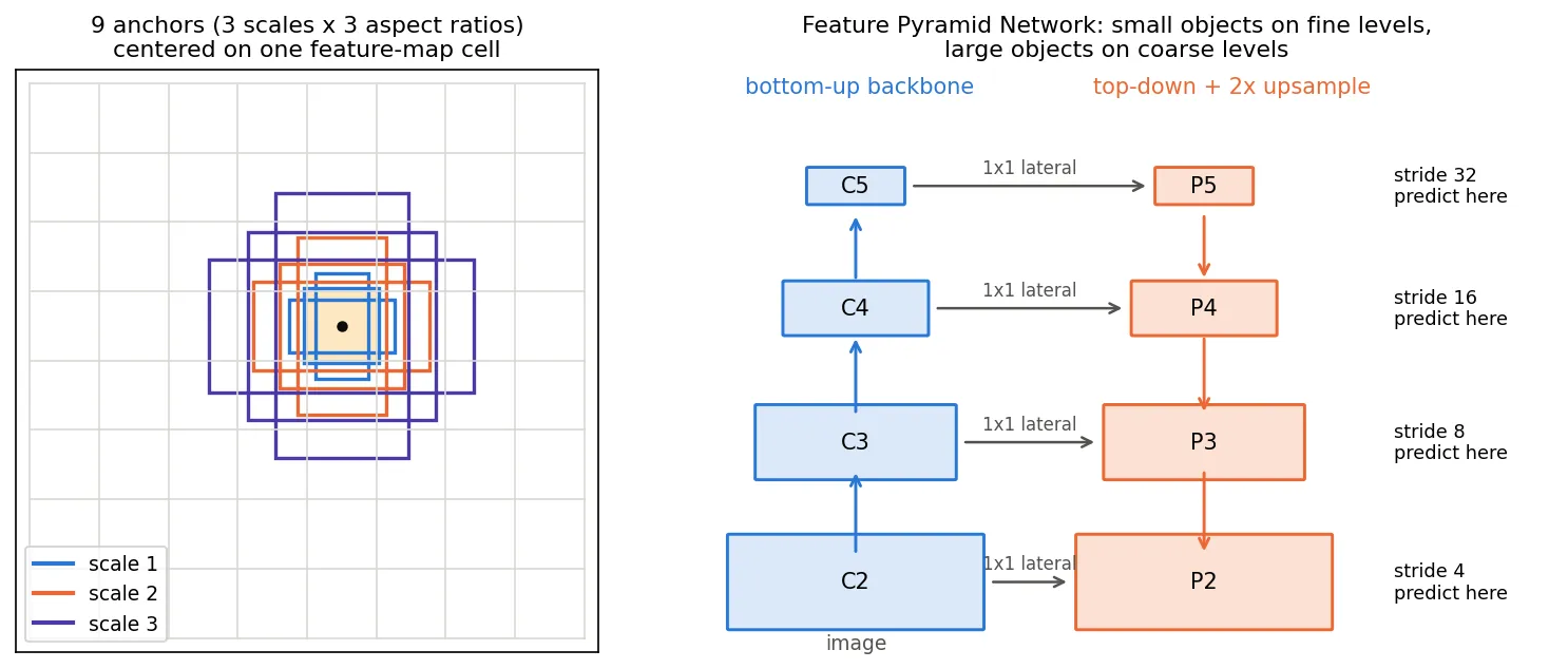
Label assignment decides which anchors are trained as which object. The classic rule is IoU-based: in the region proposal network of Faster R-CNN an anchor is positive if its IoU with some ground-truth box is at least 0.7 (or if it is the best anchor for that box), negative if its IoU with every box is below 0.3, and ignored otherwise [10]; RetinaNet uses 0.5 and 0.4 [15]. Each positive anchor regresses toward its matched box with the targets above. Assignment turned out to matter as much as architecture: anchor-free detectors (FCOS [29]) assign by location and object size instead, and DETR [30] replaces all fixed rules by a learned one-to-one matching.

Anchors have real costs: they introduce hyperparameters (scales, ratios, thresholds) that must be tuned per dataset, and they multiply the number of predictions. YOLO9000 [19] chose anchor shapes by running k-means on the training boxes, using $1 - \text{IoU}$ as the distance.

Non-maximum suppression (NMS) and Soft-NMS

Plain version. A dense detector fires many times on the same object (neighboring anchors all see it). NMS keeps the most confident box and deletes the others that overlap it too much.

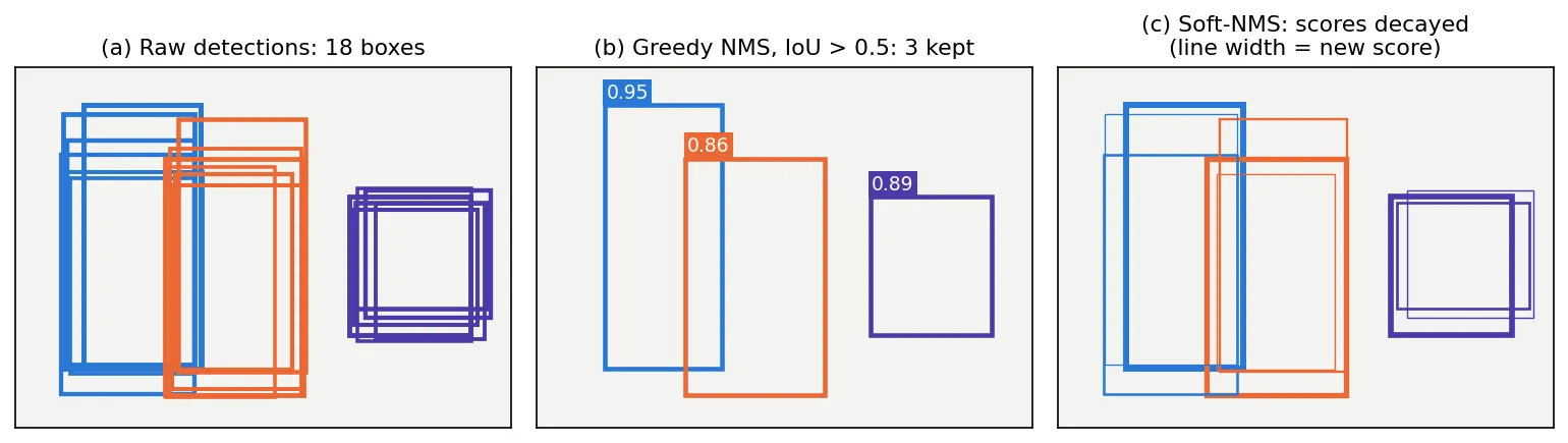
Greedy NMS, per class: sort the boxes by score; repeatedly take the highest-scoring remaining box $M$, keep it, and remove every box $b_i$ with $\text{IoU}(M, b_i) \gt N_t$ (typically $N_t = 0.5$ to $0.7$). The weakness is crowded scenes: two real people standing close may overlap by more than $N_t$, and the lower-scoring one is deleted, losing recall.

Soft-NMS [13] replaces deletion with a score decay. With the Gaussian variant,

$$s_i \leftarrow s_i \, \exp\!\left(-\frac{\text{IoU}(M, b_i)^2}{\sigma}\right),$$

where $s_i$ is the score of box $b_i$ and $\sigma$ controls how fast overlapping boxes are penalized. A heavy overlap still pushes the score down a lot, but a genuine neighbor survives with a reduced score instead of disappearing.

import numpy as np

def iou_one_to_many(box, boxes):
    x1 = np.maximum(box[0], boxes[:, 0]); y1 = np.maximum(box[1], boxes[:, 1])
    x2 = np.minimum(box[2], boxes[:, 2]); y2 = np.minimum(box[3], boxes[:, 3])
    inter = np.clip(x2 - x1, 0, None) * np.clip(y2 - y1, 0, None)
    area = lambda b: (b[..., 2] - b[..., 0]) * (b[..., 3] - b[..., 1])
    return inter / (area(box) + area(boxes) - inter)

def nms(boxes, scores, thr=0.5):
    order = np.argsort(-scores)
    keep = []
    while order.size:
        i = order[0]
        keep.append(i)
        ious = iou_one_to_many(boxes[i], boxes[order[1:]])
        order = order[1:][ious <= thr]          # drop everything that overlaps too much
    return np.array(keep)

def soft_nms(boxes, scores, sigma=0.5, score_thr=0.001):
    scores = scores.copy()
    idx = np.arange(len(scores))
    keep = []
    while idx.size:
        j = np.argmax(scores[idx]); i = idx[j]
        keep.append(i)
        idx = np.delete(idx, j)
        ious = iou_one_to_many(boxes[i], boxes[idx])
        scores[idx] *= np.exp(-ious**2 / sigma)  # decay instead of delete
        idx = idx[scores[idx] > score_thr]
    return np.array(keep), scores

# two people standing close together + duplicates
boxes = np.array([[10, 10, 60, 110], [14, 12, 62, 112], [8, 6, 58, 104],
                  [40, 15, 90, 115], [43, 18, 92, 118]], float)
scores = np.array([0.95, 0.90, 0.80, 0.85, 0.70])
print("greedy NMS keeps:", nms(boxes, scores, 0.5))
keep, s = soft_nms(boxes, scores)
print("Soft-NMS order:", keep, "rescored:", np.round(s[keep], 3))

greedy NMS keeps: [0 3]
Soft-NMS order: [0 3 2 4 1] rescored: [0.95  0.761 0.183 0.145 0.058]

Greedy NMS keeps one box per person. Soft-NMS keeps everything but ranks the duplicates far below the two real detections; a final score threshold or the AP computation then treats them as low-confidence guesses. Figure 4 shows the same effect on a synthetic scene.

NMS has three further problems: it has a hand-tuned threshold; it is a sequential, data-dependent step that is awkward to run on accelerators; and it is not part of training, so the network is never taught to avoid duplicates. Removing it is one of the main motivations behind DETR and YOLOv10 [24].

Feature pyramids (FPN)

Plain version. Small objects need high-resolution feature maps; large objects need features that have seen a lot of context. A feature pyramid gives you both, at every scale.

A CNN backbone naturally produces a pyramid $\{C_2, C_3, C_4, C_5\}$ with strides $4, 8, 16, 32$, but its shallow levels are semantically weak. The Feature Pyramid Network [14] adds a top-down path: starting from the coarsest level, it upsamples by 2 and adds a $1 \times 1$-projected lateral connection from the backbone,

$$P_l = \text{Conv}_{3\times3}\Big(\text{Conv}_{1\times1}(C_l) + \text{Up}_{2\times}(P_{l+1})\Big),$$

so every output level $P_l$ has the same channel width and strong semantics. In a two-stage detector with FPN, a region of interest of size $w \times h$ is pooled from level $l = \lfloor l_0 + \log_2(\sqrt{wh}/224) \rfloor$ (with $l_0 = 4$ in [14]), so a region twice as large moves one level up; dense detectors use a similar size-to-level rule. Later necks (extra bottom-up paths, weighted fusion) refine the same idea; nearly every detector after 2017 uses one (Figure 3, right).

Focal loss and class imbalance

Plain version. If 99.9% of your candidates are background, a normal loss is dominated by millions of easy “nothing here” examples. The focal loss turns down the volume on examples the model already gets right.

Let $p \in [0, 1]$ be the predicted probability of the foreground class and $y \in \{0, 1\}$ the label. Define $p_t = p$ if $y = 1$ and $p_t = 1 - p$ otherwise. The focal loss [15] is

$$\text{FL}(p_t) = -\alpha_t (1 - p_t)^{\gamma} \log(p_t),$$

where $\gamma \ge 0$ is the focusing parameter and $\alpha_t$ a class-balancing weight ($\alpha$ for foreground, $1 - \alpha$ for background). With $\gamma = 0$ this is weighted cross-entropy. With the paper’s default $\gamma = 2$, $\alpha = 0.25$, an easy negative with $p_t = 0.99$ is down-weighted by $(0.01)^2 = 10^{-4}$ relative to cross-entropy, while hard examples keep almost their full weight. The loss is normalized by the number of positive anchors. Two-stage detectors avoid the problem differently (the proposal stage removes most background, then a fixed foreground:background sampling ratio), and SSD [26] uses hard negative mining (keeping only the highest-loss negatives at about 3:1). The focal loss made a dense one-stage detector as accurate as two-stage ones for the first time.

Two-stage detectors: the R-CNN family

Plain version. First propose a few thousand places where something might be; then look closely at each one and decide what it is and exactly where its edges are.

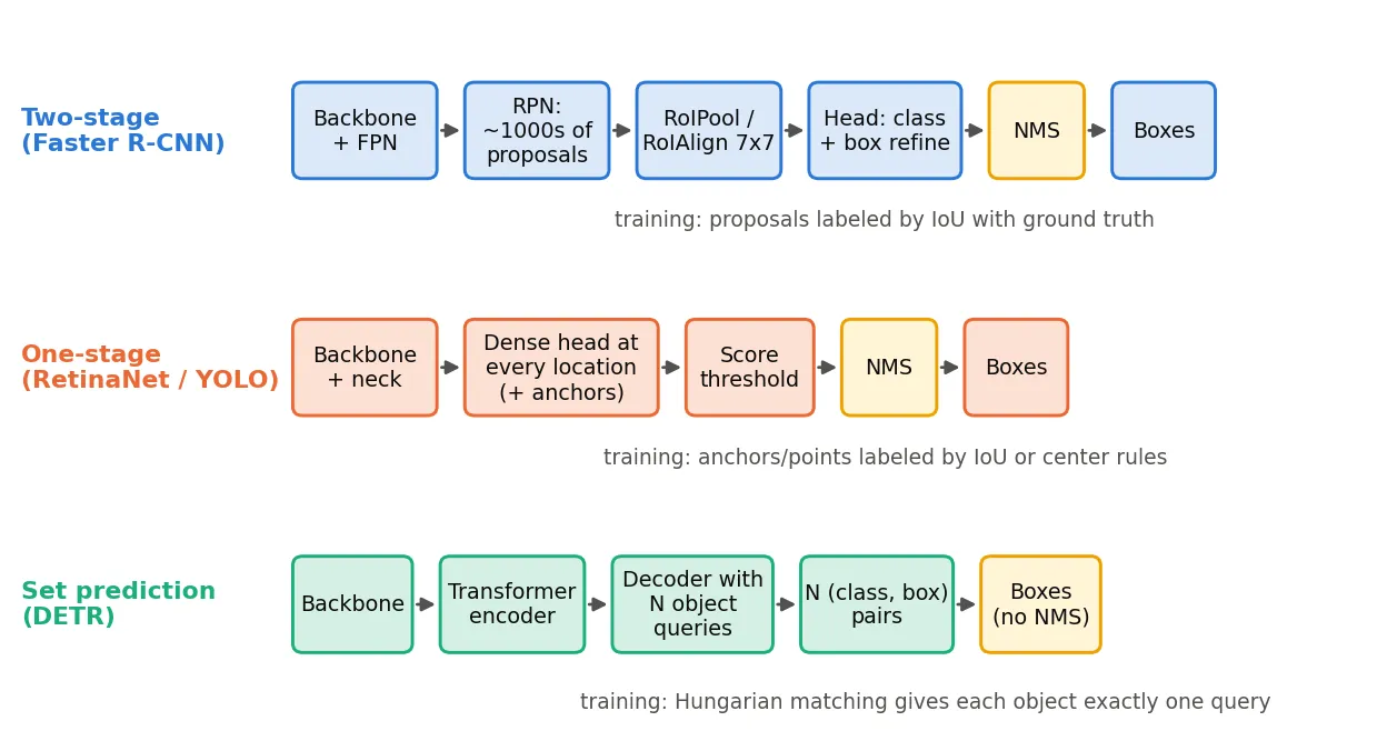
R-CNN (2014) [8] ran a bottom-up grouping algorithm to get about 2,000 class-agnostic region proposals per image, warped each one to a fixed size, passed it through a classification-pretrained CNN, scored the features with per-class linear SVMs and refined the box with the regression targets above. It improved mean AP on PASCAL VOC 2012 by more than 30% relative to the previous best result, and it established the recipe “pretrain on classification, fine-tune on detection” that is still standard. It was very slow, because the CNN ran separately on every proposal.

Fast R-CNN (2015) [9] runs the CNN once on the whole image and then crops each proposal from the shared feature map with RoI pooling: the proposal’s projection onto the feature map is divided into a fixed $H \times W$ grid (e.g. $7 \times 7$) and each bin is max-pooled, so every proposal yields the same-size feature regardless of its shape. A single network is trained with a multi-task loss,

$$L = L_{\text{cls}}(p, u) + \lambda\, [u \ge 1]\, L_{\text{loc}}(t^u, v),$$

where $p$ is the softmax over $K + 1$ classes, $u$ the true class (0 for background), $[u \ge 1]$ is 1 for foreground proposals only, $t^u$ the predicted box offsets for class $u$, $v$ the target offsets and $L_{\text{loc}}$ the smooth L1 loss.

Faster R-CNN (2015) [10] made the proposals themselves learned. A small Region Proposal Network (RPN) slides over the shared feature map and, for each of the 9 anchors per location, predicts an objectness score and box offsets. The top proposals (after NMS) feed the Fast R-CNN head. Because both stages share the backbone, proposals become almost free, and the whole detector is one network trained end to end.

Mask R-CNN (2017) [16] adds a small fully convolutional branch that predicts a binary mask per class inside each RoI, giving instance segmentation. Its key detail is RoIAlign: RoI pooling rounds the proposal boundaries and bin edges to the feature grid, which shifts features by up to half a stride. RoIAlign keeps real-valued coordinates and samples each bin with bilinear interpolation. This sounds minor, but pixel-accurate masks need it, and box accuracy at high IoU improves too.

Cascade R-CNN (2018) [17] addresses a subtle problem. A head trained with positives at IoU ≥ 0.5 learns to produce boxes that are “good at 0.5” but not at 0.75. Simply raising the threshold leaves too few positives and overfits. Cascade R-CNN chains several heads trained at increasing IoU thresholds (0.5, 0.6, 0.7), each refining the boxes of the previous one, so each stage receives a training distribution of higher quality. It was a large gain on the strict COCO metrics.

Two-stage detectors are accurate, flexible (the RoI head can predict masks, keypoints or attributes) and still the default for many instance-segmentation tasks, but the per-RoI head and NMS cost time.

One-stage detectors: YOLO, SSD and RetinaNet

Plain version. Skip the proposal step. Make one dense prediction at every location of the feature map in a single forward pass, then clean it up with NMS.

YOLO v1 (2016) [18] divided the image into an $S \times S$ grid ($S = 7$). Each cell predicted $B = 2$ boxes, each with a confidence, plus one set of $C$ class probabilities, so the output was a single $S \times S \times (5B + C)$ tensor ($7 \times 7 \times 30$ for PASCAL VOC’s 20 classes). The cell containing an object’s center was responsible for it. It ran in real time and, because it saw the whole image, made fewer background errors than Fast R-CNN, but it localized less precisely and struggled with small objects and groups, since each cell could only predict a fixed number of boxes and one class.

The YOLO family then evolved quickly. The table lists only versions with a paper we could verify; many widely used releases are maintained as software packages without papers and are not covered here.

Version	Year	Main ideas (from the paper)
YOLO [18]	2016	Single-pass grid regression; real time
YOLO9000 / v2 [19]	2016 (arXiv)	Anchors chosen by k-means with an IoU distance; batch norm; higher-resolution training
YOLOv3 [20]	2018 (tech report)	Deeper backbone; predictions at three scales; independent logistic class scores
YOLOv4 [21]	2020 (arXiv)	Systematic study of training tricks (“bag of freebies”) and cheap architectural add-ons (“bag of specials”)
YOLOv7 [22]	2023 (CVPR)	Trainable bag-of-freebies: re-parameterized modules, improved label assignment, efficient layer aggregation
YOLOv9 [23]	2024 (ECCV)	Programmable gradient information (PGI) to keep information through deep layers; GELAN backbone
YOLOv10 [24]	2024 (NeurIPS)	NMS-free training with consistent dual (one-to-many and one-to-one) assignments; efficiency-driven design
YOLOv12 [25]	2025 (arXiv)	Attention-centric design that keeps real-time speed

A recurring theme is visible: the core “dense grid + NMS” idea stayed, while label assignment, necks, training recipes and, most recently, attention and NMS-free heads changed.

SSD (2016) [26] attached small convolutional predictors to several feature maps of different resolutions, each with its own set of default boxes (anchors) of several aspect ratios, which handled scale far better than YOLO v1. It trained with hard negative mining and heavy data augmentation.

RetinaNet (2017) [15] combined an FPN backbone, dense anchors (9 per location) and two small subnetworks for classification and box regression, trained with the focal loss. The paper’s analysis showed that class imbalance, not the architecture, had been the main reason one-stage detectors lagged behind two-stage ones.

Anchor-free detectors: points instead of boxes

Plain version. Anchors are guesses about what objects look like. Anchor-free detectors drop them and predict boxes from points: corners, centers, or every pixel inside the object.

CornerNet (2018) [27] detects an object as a pair of keypoints: a heatmap for top-left corners, a heatmap for bottom-right corners, and an embedding per corner. Corners from the same object are trained to have similar embeddings, so pairing is done by embedding distance. Because a corner often lies outside the object, the paper introduced corner pooling, which looks along rows and columns to collect evidence for a corner.

CenterNet, “Objects as Points” (2019) [28] represents each object by its center. The network outputs a heatmap $\hat{Y} \in [0, 1]^{\frac{W}{R} \times \frac{H}{R} \times K}$ (output stride $R$, one channel per class), plus a size $(w, h)$ and a sub-pixel offset at each location. Ground-truth centers are splatted with a Gaussian, and the heatmap is trained with a pixel-wise focal loss. At inference, peaks are simply local maxima, found with a $3 \times 3$ max-pooling comparison, so no IoU-based NMS is needed. The same design extends to 3D boxes and human pose by regressing more quantities at the center.

FCOS (2019) [29] treats detection like segmentation. Every feature-map location that falls inside a ground-truth box is a positive sample and regresses the four distances to the box sides,

$$l^* = x - x_1, \qquad t^* = y - y_1, \qquad r^* = x_2 - x, \qquad b^* = y_2 - y,$$

where $(x, y)$ is the location in image coordinates and $(x_1, y_1, x_2, y_2)$ the box. Each FPN level only handles objects whose largest regression distance falls in its own range, which resolves most ambiguity when boxes overlap. Locations far from the object’s center produce poor boxes, so FCOS adds a centerness branch,

$$\text{centerness} = \sqrt{\frac{\min(l^*, r^*)}{\max(l^*, r^*)} \cdot \frac{\min(t^*, b^*)}{\max(t^*, b^*)}},$$

that is 1 at the center and decays toward the edges; it multiplies the class score at test time so off-center boxes rank lower before NMS. FCOS removed every anchor hyperparameter and matched or beat anchor-based RetinaNet.

Set prediction with transformers: DETR and its descendants

Plain version. Instead of predicting thousands of candidates and deleting duplicates, predict a small set of answers directly, and train so that each real object is claimed by exactly one prediction.

DETR (2020) [30] uses a CNN backbone, a transformer encoder over the feature map, and a transformer decoder that takes $N$ learned object queries (100 in the paper) and outputs $N$ (class, box) predictions in parallel. There are no anchors, no proposals and no NMS. Since $N$ exceeds the number of objects, a special “no object” class $\varnothing$ pads the ground truth to size $N$.

The key is training with bipartite matching. Let $y = \{y_j\}$ be the padded ground truth and $\hat{y} = \{\hat{y}_i\}_{i=1}^{N}$ the predictions. Find the permutation $\hat{\sigma}$ of $N$ elements with lowest total matching cost,

$$\hat{\sigma} = \arg\min_{\sigma \in \mathfrak{S}_N} \sum_{j=1}^{N} \mathcal{L}_{\text{match}}\big(y_j, \hat{y}_{\sigma(j)}\big), \qquad \mathcal{L}_{\text{match}} = -\mathbb{1}_{\{c_j \ne \varnothing\}}\, \hat{p}_{\sigma(j)}(c_j) + \mathbb{1}_{\{c_j \ne \varnothing\}}\, \mathcal{L}_{\text{box}}\big(b_j, \hat{b}_{\sigma(j)}\big),$$

where $\mathfrak{S}_N$ is the set of permutations, $c_j$ and $b_j$ are the class and box of target $j$, $\hat{p}_{\sigma(j)}(c_j)$ is the predicted probability of class $c_j$ for the matched query, and $\mathcal{L}_{\text{box}} = \lambda_{L1} \lVert b_j - \hat{b}_{\sigma(j)} \rVert_1 + \lambda_{\text{iou}} \big(1 - \text{GIoU}(b_j, \hat{b}_{\sigma(j)})\big)$. This assignment problem is solved exactly by the Hungarian algorithm [31] in polynomial time. The training loss (the set loss) then uses the matched pairs:

$$\mathcal{L}_{\text{Hungarian}} = \sum_{j=1}^{N} \Big[ -\log \hat{p}_{\hat{\sigma}(j)}(c_j) + \mathbb{1}_{\{c_j \ne \varnothing\}}\, \mathcal{L}_{\text{box}}\big(b_j, \hat{b}_{\hat{\sigma}(j)}\big) \Big],$$

with the log-probability term down-weighted by a factor of 10 for $c_j = \varnothing$ to balance the many “no object” slots. Because each object is matched to exactly one query, a duplicate prediction is penalized as a false “no object”, and the decoder’s self-attention learns to suppress duplicates, which is why NMS is unnecessary.

The matching step is short with SciPy. The cost below combines the three terms with DETR’s weights; linear_sum_assignment accepts the rectangular $N \times M$ matrix directly (DETR computes the L1 term on normalized $(c_x, c_y, w, h)$; corner format is used here for brevity).

import numpy as np
from scipy.optimize import linear_sum_assignment

def giou_matrix(a, b):
    x1 = np.maximum(a[:, None, 0], b[None, :, 0]); y1 = np.maximum(a[:, None, 1], b[None, :, 1])
    x2 = np.minimum(a[:, None, 2], b[None, :, 2]); y2 = np.minimum(a[:, None, 3], b[None, :, 3])
    inter = np.clip(x2 - x1, 0, None) * np.clip(y2 - y1, 0, None)
    area = lambda b: (b[:, 2] - b[:, 0]) * (b[:, 3] - b[:, 1])
    union = area(a)[:, None] + area(b)[None, :] - inter
    cx1 = np.minimum(a[:, None, 0], b[None, :, 0]); cy1 = np.minimum(a[:, None, 1], b[None, :, 1])
    cx2 = np.maximum(a[:, None, 2], b[None, :, 2]); cy2 = np.maximum(a[:, None, 3], b[None, :, 3])
    c = (cx2 - cx1) * (cy2 - cy1)
    return inter / union - (c - union) / c

rng = np.random.default_rng(1)
N, C = 6, 3                                     # 6 queries, 3 real classes (+ "no object")
logits = rng.normal(size=(N, C + 1))
prob = np.exp(logits) / np.exp(logits).sum(1, keepdims=True)
pred_boxes = np.array([[.10, .10, .40, .50], [.55, .20, .90, .60], [.12, .08, .42, .48],
                       [.30, .60, .60, .95], [.00, .00, .20, .20], [.50, .50, .70, .70]])
gt_boxes  = np.array([[.10, .10, .40, .50], [.32, .62, .62, .93], [.56, .22, .88, .62]])
gt_labels = np.array([0, 2, 1])

w_cls, w_l1, w_giou = 1.0, 5.0, 2.0             # weights used by DETR
cost = (-w_cls * prob[:, gt_labels]                          # (N, M) class term
        + w_l1 * np.abs(pred_boxes[:, None] - gt_boxes[None]).sum(-1)
        - w_giou * giou_matrix(pred_boxes, gt_boxes))
rows, cols = linear_sum_assignment(cost)        # works on rectangular N x M matrices
print("query -> gt:", dict(zip(rows.tolist(), cols.tolist())))
print("unmatched queries (trained as 'no object'):", sorted(set(range(N)) - set(rows.tolist())))

query -> gt: {0: 0, 1: 2, 3: 1}
unmatched queries (trained as 'no object'): [2, 4, 5]

Query 2 is a near-duplicate of query 0, yet it is left unmatched and will be trained toward “no object”. That is the mechanism that replaces NMS.

The price. DETR needed very long training schedules (hundreds of epochs, compared with roughly a dozen for Faster R-CNN) and was weak on small objects, because global attention over a high-resolution feature map is expensive, so it used only a single coarse level. The descendants fixed these problems one by one.

• Deformable DETR (2021) [32] replaces dense attention with deformable attention: each query attends to only a few learned sampling points around a reference point, across multiple feature levels. This makes multi-scale features affordable and, according to the paper, reaches better accuracy than DETR (especially on small objects) with 10 times fewer training epochs.
• DINO (2022) [33] (not to be confused with the self-supervised method of the same name) combines contrastive denoising training (noised copies of ground-truth boxes are fed as extra queries and must be reconstructed, while slightly more noised ones must be rejected), mixed query selection (initializing anchor positions from encoder features) and a look-forward-twice box update. It reports 49.4 AP after 12 epochs and 51.3 AP after 24 epochs on COCO with a standard 50-layer CNN backbone, and 63.2 AP on COCO val2017 with a large backbone and Objects365 pretraining.
• RT-DETR (2024) [34] targets real-time use. An efficient hybrid encoder applies attention only to the coarsest level and fuses scales with convolutions, and IoU-aware query selection picks better initial queries. The paper reports 53.1 / 54.3 AP on COCO at 108 / 74 FPS on a T4 GPU for its smaller and larger variants, faster and more accurate than YOLO models of comparable size at the time, without NMS.

Today the DETR line and the YOLO line are converging: YOLOv10 borrows one-to-one assignment to drop NMS, and real-time DETRs borrow efficient convolutional necks.

Open-vocabulary and grounding detectors

Plain version. A closed-set detector can only find the 80 or 365 classes it was trained on. An open-vocabulary detector takes the class list as text at test time, so you can ask for “red fire hydrant” or “forklift” without retraining.

The trick is to replace the last classification layer, a fixed matrix of $K$ class weight vectors, with text embeddings. For a region feature $\mathbf{z}_i$ and the text embedding $\mathbf{e}_k$ of a prompt such as “a photo of a forklift”, the class score is a scaled cosine similarity,

$$s_{ik} = \tau \cdot \frac{\mathbf{z}_i^\top \mathbf{e}_k}{\lVert \mathbf{z}_i \rVert \, \lVert \mathbf{e}_k \rVert},$$

where $\tau$ is a learned temperature. Any phrase you can embed becomes a class. The vision side must learn to align regions with language, which requires image–text data far larger than any box-annotated dataset.

• OWL-ViT (2022) [35] starts from a transformer image encoder and a text encoder pretrained contrastively on image–text pairs, removes the final pooling, and attaches light box and class heads to every output token. The class head is the text embedding above. It supports zero-shot (text query) and one-shot (image-exemplar query) detection, and the paper shows consistent gains with model scale.
• Grounding DINO (2024) [36] fuses language deeply into a DINO detector: a feature enhancer with cross-attention between image and text, language-guided query selection, and a cross-modality decoder. It is pretrained on detection, grounding (phrase-to-region) and caption data, and reports 52.5 AP on COCO zero-shot transfer (with no COCO training data) and a 26.1 mean AP on a benchmark collection of diverse real-world detection datasets.
• YOLO-World (2024) [37] brings open vocabulary to real-time detectors with a vision–language path aggregation network (RepVL-PAN) and region–text contrastive pretraining. Its prompt-then-detect mode encodes the user’s vocabulary once offline, so inference costs about the same as a closed-set YOLO. It reports 35.4 AP on LVIS at 52.0 FPS on a V100 GPU.

Promptable foundation models go one step further. SAM 3 [38] (2025) accepts a short noun phrase or image exemplars as a concept prompt and returns masks with identities for all matching instances in images and videos; the authors built a data engine producing a dataset with 4M unique concept labels and report doubling the accuracy of existing systems on their promptable concept segmentation benchmark. In such systems, detection becomes one output of a general “find this concept” model rather than a separately trained network.

Small objects and dense scenes

Plain version. Tiny objects have very few pixels, and stride-32 features may squeeze them into less than one cell. Crowds are hard because objects hide each other and NMS confuses neighbors with duplicates.

Small objects. COCO defines “small” as area below $32^2$ pixels [40]. After a stride-16 backbone, such an object covers at most about $2 \times 2$ feature cells, and its appearance is mostly lost in downsampling. IoU also becomes harsh: a 2-pixel error on a $10 \times 10$ box can drop IoU below 0.7. Common remedies are high-resolution feature levels ($P_2$ with stride 4), feature pyramids, image tiling or slicing at inference, larger input resolutions, copy-paste and scale augmentation, and assignment rules that do not starve small boxes of positive samples. The survey and benchmark of Cheng et al. [39] reviews these strategies and introduces two large small-object benchmarks: SODA-D (24,828 traffic images, 278,433 instances, 9 categories) and SODA-A (2,513 high-resolution aerial images, 872,069 instances, 9 classes).

Dense and occluded scenes. In crowds, true objects overlap heavily, so a fixed NMS threshold trades recall against duplicates. Soft-NMS [13] helps; set-prediction detectors avoid the threshold altogether by learning which predictions are duplicates. Occlusion also makes box annotation ambiguous (full extent or visible part?), and evaluation then depends on the protocol. These issues return in tracking, where objects disappear and reappear.

Evaluating detectors

Plain version. Sort all detections by confidence. Walk down the list: each detection is either a hit (it matches an unclaimed real object well enough) or a false alarm. Track how precision and recall change; the area under that curve is the Average Precision.

Precision, recall and AP

For one class and one IoU threshold $\theta$, sort all detections in the test set by descending score. A detection is a true positive (TP) if its IoU with a not-yet-matched ground-truth box of the same class is at least $\theta$; otherwise it is a false positive (FP). Each ground-truth box can be matched only once, which is how duplicates are punished. After the top $k$ detections,

$$\text{precision}(k) = \frac{\text{TP}(k)}{k}, \qquad \text{recall}(k) = \frac{\text{TP}(k)}{M},$$

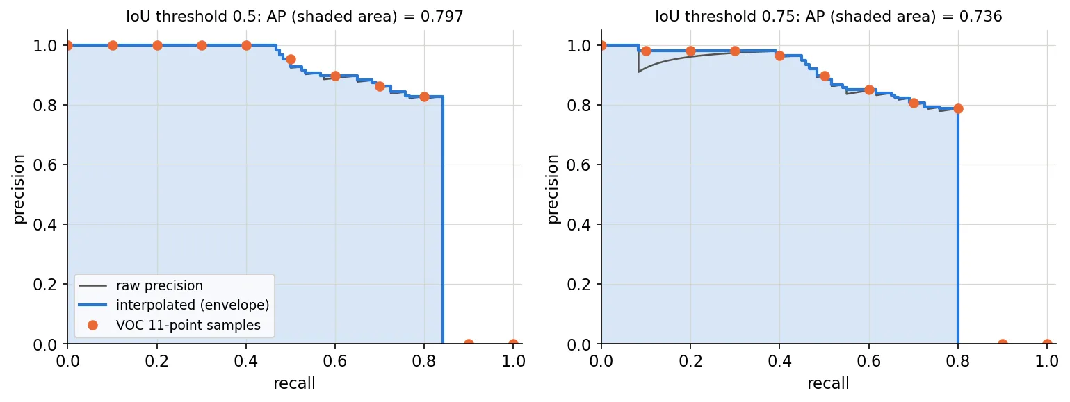
where $M$ is the number of ground-truth objects of that class. To make the curve monotone, precision is interpolated with its upper envelope, $p_{\text{interp}}(r) = \max_{r' \ge r} p(r')$. Then:

• VOC 11-point AP (PASCAL VOC up to 2009 [3]): $\text{AP} = \frac{1}{11} \sum_{r \in \{0, 0.1, \dots, 1\}} p_{\text{interp}}(r)$.
• VOC all-point AP (VOC 2010 onwards [41]): the exact area under the interpolated curve, $\text{AP} = \sum_n (r_{n+1} - r_n)\, p_{\text{interp}}(r_{n+1})$ over the distinct recall values.
• COCO AP [40]: the mean of $p_{\text{interp}}$ at 101 recall points $0, 0.01, \dots, 1$.

Figure 6 shows a PR curve, its envelope and the AP area.

The COCO protocol

COCO’s primary metric, written AP or mAP@[.5:.95], averages AP over 10 IoU thresholds $\theta \in \{0.50, 0.55, \dots, 0.95\}$ and over all 80 categories [40]:

$$\text{AP}_{\text{COCO}} = \frac{1}{10\,K} \sum_{\theta} \sum_{k=1}^{K} \text{AP}_k(\theta).$$

It rewards precise localization, not just finding the object. Companion metrics are $\text{AP}_{50}$ (the VOC-style metric), $\text{AP}_{75}$ (strict), and $\text{AP}_S$, $\text{AP}_M$, $\text{AP}_L$ for small (area $\lt 32^2$), medium ($32^2$ to $96^2$) and large ($\gt 96^2$) objects. At most 100 detections per image are scored. Average recall (AR) at 1, 10 and 100 detections per image is also reported. Note that COCO calls its category-averaged metric “AP”; “mAP” in papers usually means the same thing.

The code below computes everything from scratch on synthetic predictions (jittered ground truth, about 15% misses and some random false positives).

import numpy as np

def box_iou(a, b):
    """Pairwise IoU between (N,4) and (M,4) xyxy boxes -> (N, M)."""
    x1 = np.maximum(a[:, None, 0], b[None, :, 0]); y1 = np.maximum(a[:, None, 1], b[None, :, 1])
    x2 = np.minimum(a[:, None, 2], b[None, :, 2]); y2 = np.minimum(a[:, None, 3], b[None, :, 3])
    inter = np.clip(x2 - x1, 0, None) * np.clip(y2 - y1, 0, None)
    area = lambda b: (b[:, 2] - b[:, 0]) * (b[:, 3] - b[:, 1])
    return inter / (area(a)[:, None] + area(b)[None, :] - inter)

def match(dets, gts, thr):
    """dets: list over images of (boxes, scores); gts: list of gt boxes.
    Returns scores, TP flags (sorted by score), and number of GT."""
    recs = []
    for img, ((db, ds), gb) in enumerate(zip(dets, gts)):
        for k in range(len(ds)):
            recs.append((ds[k], img, k))
    recs.sort(key=lambda r: -r[0])                       # global ranking by confidence
    used = [np.zeros(len(g), bool) for g in gts]
    tp = np.zeros(len(recs))
    for n, (s, img, k) in enumerate(recs):
        gb = gts[img]
        if len(gb) == 0:
            continue
        ious = box_iou(dets[img][0][k:k + 1], gb)[0]
        ious[used[img]] = -1                             # each GT can be matched once
        j = ious.argmax()
        if ious[j] >= thr:
            tp[n] = 1; used[img][j] = True
    return tp, sum(len(g) for g in gts)

def pr_curve(tp, n_gt):
    ctp, cfp = np.cumsum(tp), np.cumsum(1 - tp)
    return ctp / n_gt, ctp / (ctp + cfp)                 # recall, precision

def ap(rec, prec, mode="all"):
    r = np.concatenate([[0], rec, [1]]); p = np.concatenate([[0], prec, [0]])
    p = np.maximum.accumulate(p[::-1])[::-1]             # monotone envelope
    if mode == "all":                                    # VOC2010+: exact area
        i = np.where(r[1:] != r[:-1])[0]
        return np.sum((r[i + 1] - r[i]) * p[i + 1])
    pts = np.linspace(0, 1, 11 if mode == "voc11" else 101)
    return np.mean([p[r >= t].max() if np.any(r >= t) else 0 for t in pts])

# synthetic data: 50 images, 1-4 objects each; detector = jittered GT + false positives
rng = np.random.default_rng(0)
gts, dets = [], []
for _ in range(50):
    n = rng.integers(1, 5)
    xy = rng.uniform(0, 200, (n, 2)); wh = rng.uniform(20, 80, (n, 2))
    g = np.hstack([xy, xy + wh]); gts.append(g)
    keep = rng.random(n) > 0.15                          # miss ~15% of objects
    jit = rng.normal(0, 0.06, (n, 4)) * np.hstack([wh, wh])
    db = (g + jit)[keep]; ds = rng.uniform(0.4, 1.0, keep.sum())
    m = rng.integers(0, 3)                               # 0-2 false positives
    fxy = rng.uniform(0, 200, (m, 2)); fwh = rng.uniform(20, 80, (m, 2))
    db = np.vstack([db, np.hstack([fxy, fxy + fwh])]); ds = np.concatenate([ds, rng.uniform(0, 0.7, m)])
    dets.append((db, ds))

for thr in (0.5, 0.75):
    tp, n_gt = match(dets, gts, thr)
    rec, prec = pr_curve(tp, n_gt)
    print(f"IoU {thr}: VOC11 {ap(rec, prec, 'voc11'):.3f}  all-point {ap(rec, prec):.3f}"
          f"  COCO-101 {ap(rec, prec, 'coco'):.3f}")
aps = [ap(*pr_curve(*match(dets, gts, t)), "coco") for t in np.arange(0.5, 0.96, 0.05)]
print("AP@[.5:.95] =", round(float(np.mean(aps)), 3))

IoU 0.5: VOC11 0.776  all-point 0.797  COCO-101 0.797
IoU 0.75: VOC11 0.749  all-point 0.736  COCO-101 0.738
AP@[.5:.95] = 0.532

Three lessons are visible. The three interpolation rules give similar but not identical numbers, so AP values computed with different protocols must never be compared. AP@[.5:.95] is much lower than AP50 because jittered boxes fail the strict thresholds. And this is a single class; real mAP averages over classes, so rare classes count as much as frequent ones.

What AP does not tell you

AP summarizes ranking quality over the whole test set, so it does not choose an operating threshold, and it does not separate types of errors: localization errors, confusion with similar classes, duplicates and background false positives all look the same. When diagnosing a model, break errors down by type and by object size, and look at the images.

Datasets and benchmarks

Plain version. Detection progress has been driven by a few public datasets; each one changed what “good” meant.

Dataset	Classes	Scale (from the papers)	Annotations	Why it matters
PASCAL VOC [3]	20	Small by today’s standards	Boxes (+ some masks)	The 2005–2012 benchmark; AP50
MS COCO [4]	91 types labeled; 80 used for detection	328k images, 2.5M labeled instances	Boxes + instance masks	Cluttered everyday scenes, many small objects; AP@[.5:.95]
Objects365 [42]	365	Large-scale, high-quality boxes	Boxes	Common pretraining set for strong detectors
Open Images V4 [43]	600 boxable classes	9.2M images; 15.4M boxes	Boxes, image labels, relationships	Very large; 19.8k concepts at image level
LVIS [44]	over 1000	~2M masks in 164k images	Instance masks	Long-tailed vocabulary; rare-class evaluation

Two trends stand out. Category counts grew (20, then 80, then hundreds and over a thousand), and with them came long-tail problems: in LVIS many categories have only a handful of training examples, so a loss or sampler that ignores frequency fails on rare classes. And the biggest models are now pretrained on Objects365 or on image–text data before fine-tuning on COCO, which makes “trained on COCO only” and “with extra data” separate leaderboards.

Speed, accuracy and deployment

Plain version. In practice you pick a point on a curve: more accuracy usually means more computation. What counts is the latency on your hardware, end to end.

• FLOPs are not latency. FLOPs count arithmetic, but runtime also depends on memory traffic, operator support and parallelism. Depth-wise convolutions and attention can be cheap in FLOPs but slow on some accelerators.
• Measure end to end. Report latency including preprocessing, the network and post-processing. NMS cost grows with the number of candidate boxes (worst case quadratic in their number), is data-dependent, and often runs on the CPU. RT-DETR’s paper [34] analyses exactly this and is one reason NMS-free designs such as RT-DETR and YOLOv10 [24] are attractive for deployment.
• Input resolution is the strongest knob: halving the side length cuts compute by about 4 times but hurts small objects most.
• Quantization (e.g. 8-bit integer weights and activations) and re-parameterization (training a multi-branch block, then folding it into a single convolution, as used by YOLOv7 [22]) reduce latency with small accuracy loss. Box-regression outputs and the score head are often the most sensitive to quantization, so calibrate with real data and check AP75, not just AP50.
• Batch size 1 is the usual edge setting; throughput numbers measured with large batches do not transfer.

A tiny detector you can train

To see box regression and an IoU loss work end to end, the PyTorch script below trains a small CNN to localize one rectangle or ellipse in noisy $32 \times 32$ images. It is a single-object detector: the network directly regresses $(c_x, c_y, w, h)$ in $[0, 1]$ through a sigmoid, trained with L1 plus a GIoU loss, as DETR does for its matched queries.

import time, torch, torch.nn as nn
torch.manual_seed(0)
S = 32
torch.set_num_threads(4)

def make_batch(n):
    """One white rectangle or ellipse per 32x32 noisy image; target = (cx, cy, w, h) in [0, 1]."""
    img = 0.1 * torch.randn(n, 1, S, S)
    wh = torch.rand(n, 2) * 0.4 + 0.15
    c = wh / 2 + torch.rand(n, 2) * (1 - wh)
    yy, xx = torch.meshgrid(torch.arange(S), torch.arange(S), indexing="ij")
    xx, yy = (xx[None] + 0.5) / S, (yy[None] + 0.5) / S
    dx = (xx - c[:, 0, None, None]) / (wh[:, 0, None, None] / 2)
    dy = (yy - c[:, 1, None, None]) / (wh[:, 1, None, None] / 2)
    rect = (dx.abs() <= 1) & (dy.abs() <= 1)
    ell = dx**2 + dy**2 <= 1
    shape = torch.where((torch.rand(n) < 0.5)[:, None, None], rect, ell)
    return img + shape[:, None].float(), torch.cat([c, wh], 1)

def xyxy(b):
    return torch.cat([b[:, :2] - b[:, 2:] / 2, b[:, :2] + b[:, 2:] / 2], 1)

def giou(p, g):
    p, g = xyxy(p), xyxy(g)
    lt, rb = torch.max(p[:, :2], g[:, :2]), torch.min(p[:, 2:], g[:, 2:])
    inter = (rb - lt).clamp(min=0).prod(1)
    area = lambda b: (b[:, 2:] - b[:, :2]).prod(1)
    union = area(p) + area(g) - inter
    c = (torch.max(p[:, 2:], g[:, 2:]) - torch.min(p[:, :2], g[:, :2])).prod(1)
    return inter / union, inter / union - (c - union) / c

net = nn.Sequential(
    nn.Conv2d(1, 16, 3, padding=1), nn.ReLU(), nn.MaxPool2d(2),   # 16
    nn.Conv2d(16, 32, 3, padding=1), nn.ReLU(), nn.MaxPool2d(2),  # 8
    nn.Conv2d(32, 32, 3, padding=1), nn.ReLU(), nn.MaxPool2d(2),  # 4
    nn.Flatten(), nn.Linear(32 * 4 * 4, 128), nn.ReLU(),
    nn.Linear(128, 4), nn.Sigmoid())                               # (cx, cy, w, h) in [0, 1]
opt = torch.optim.Adam(net.parameters(), 2e-3)

t0 = time.time()
for step in range(500):
    x, y = make_batch(64)
    pred = net(x)
    iou, g = giou(pred, y)
    loss = (pred - y).abs().sum(1).mean() + (1 - g).mean()        # L1 + GIoU loss
    opt.zero_grad(); loss.backward(); opt.step()

with torch.no_grad():
    x, y = make_batch(1000)
    iou, _ = giou(net(x), y)
print(f"train time {time.time() - t0:.1f}s | test mean IoU {iou.mean():.3f}"
      f" | IoU>=0.5: {(iou >= 0.5).float().mean():.1%} | IoU>=0.75: {(iou >= 0.75).float().mean():.1%}")

train time 21.1s | test mean IoU 0.885 | IoU>=0.5: 100.0% | IoU>=0.75: 97.8%

(Training time depends on your CPU.) Because there is exactly one object, there is no assignment and no NMS. Exercise 6 asks you to extend this to several objects, which is where every hard problem in this tutorial reappears.

Modern view

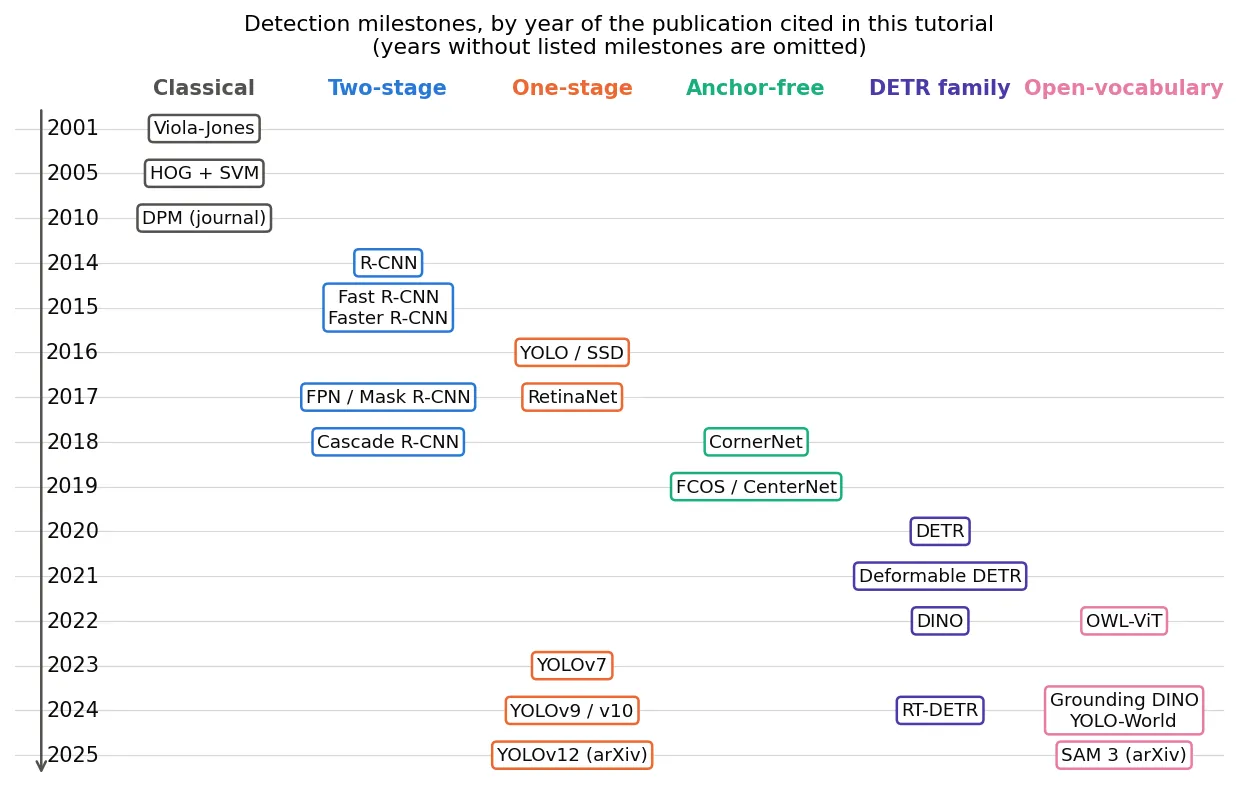
Figure 7 places the methods of this tutorial on a timeline, using the year of each cited publication.

What the surveys say

Object Detection in 20 Years (Zou et al., Proceedings of the IEEE, 2023) [1] is the broadest historical review. It covers milestone detectors from the traditional era (Viola–Jones, HOG, DPM) to deep two-stage and one-stage methods, detection datasets and metrics, fundamental building blocks (multi-scale detection, context, hard-negative mining, NMS, box regression), speed-up techniques, and recent state-of-the-art methods. Its main message is that most “new” ideas have older roots: multi-scale scanning became feature pyramids, cascades became cascaded heads, hard-negative mining became the focal loss, and NMS has been rethought several times.

Deep Learning for Generic Object Detection: A Survey (Liu et al., IJCV, 2020) [2] reviews over 300 contributions in depth and organizes them by detection framework, object feature representation, object proposal generation, context modeling, training strategies and evaluation metrics. It is the best single reference for the pre-transformer CNN era, and it stresses that progress came as much from training strategies, data and evaluation as from architectures.

Object Detection with Transformers: A Review (Shehzadi et al., Sensors, 2025) [45] analyses 21 recent improvements to DETR, grouped by changes to the backbone, query design and attention mechanism, and compares them on common benchmarks. Its taxonomy tracks the fixes described above: multi-scale and sparse attention for small objects and speed, and better query initialization and denoising for convergence.

A Survey on Open-Vocabulary Detection and Segmentation: Past, Present, and Future (Zhu and Chen, IEEE TPAMI, 2024) [46] organizes open-vocabulary methods by how they use weak supervision into six families: visual–semantic space mapping, novel visual feature synthesis, region-aware training, pseudo-labeling, knowledge distillation and transfer learning. It covers 2D, 3D and video tasks, and it highlights how evaluation of “novel” classes is complicated by vocabulary overlap between pretraining and test data.

Towards Large-Scale Small Object Detection (Cheng et al., IEEE TPAMI, 2023) [39] focuses on the most stubborn failure mode, reviews the remedies by category and contributes the SODA benchmarks described earlier. It shows that small-object accuracy remains far below that of larger objects even for strong detectors.

The state of the art, 2023–2026

• Real-time closed-set detection is now a contest between the YOLO line (YOLOv9 [23], YOLOv10 [24], YOLOv12 [25]) and real-time DETRs (RT-DETR [34]). The two lines borrow from each other: one-to-one assignment and NMS-free heads in YOLO, convolutional necks and hybrid encoders in DETRs. Attention is now affordable at real-time budgets.
• High-accuracy closed-set detection is dominated by DETR-style models such as DINO [33] with large backbones and large-scale pretraining (Objects365 [42] and beyond). Gains on COCO have become small, and the benchmark is close to saturated for the largest models, which is pushing attention to harder benchmarks: LVIS [44], open vocabulary and cross-domain evaluation.
• Open-vocabulary and grounding detection (OWL-ViT [35], Grounding DINO [36], YOLO-World [37]) is moving into practice: in many applications you now prompt a detector rather than train one, and then optionally fine-tune it.
• Promptable foundation models (SAM 3 [38]) unify detection, segmentation and tracking under concept prompts.

Open problems

1. Localization quality versus confidence. Classification score and box quality are trained separately and are often poorly correlated, so the “best” box can be suppressed by a more confident but worse one.
2. Small, crowded and occluded objects remain far from solved [39].
3. Long-tail and open-world recognition. Rare classes and truly unseen objects, and knowing when the model does not know.
4. Evaluation. COCO AP hides error types, is saturated at the top, and open-vocabulary evaluation depends on prompts and on what the pretraining data already contained [46].
5. Efficiency on real hardware, including NMS-free designs, quantization-friendly heads and fair latency reporting.

Key takeaways

• Detection outputs a variable-size set of (box, class, score) triples; every architecture is a different answer to “how many, and which one is responsible for which object?”
• Boxes are regressed as scale-normalized offsets from a reference ($t_x, t_y, \log$-scale $t_w, t_h$); IoU-based losses (GIoU, DIoU, CIoU) align training with the IoU-based metric.
• Anchors and assignment rules decide which predictions learn which object; NMS removes duplicates afterwards, and Soft-NMS softens its failure in crowds.
• FPN handles scale; the focal loss handles the foreground–background imbalance that made dense detectors weak.
• Two-stage (R-CNN, Fast, Faster, Mask, Cascade) refine proposals; one-stage (YOLO, SSD, RetinaNet) predict densely in one pass; anchor-free (CornerNet, CenterNet, FCOS) predict from points; DETR predicts a set with Hungarian matching and needs no NMS.
• Open-vocabulary detectors turn the class list into text prompts, and promptable foundation models merge detection, segmentation and tracking.
• Measure with the right protocol: VOC 11-point, VOC all-point and COCO 101-point AP differ; COCO AP averages IoU 0.50–0.95, and APs/m/l expose scale weaknesses.

Exercises

1. Encode by hand. An anchor has center $(100, 100)$ and size $64 \times 32$. A ground-truth box has center $(110, 96)$ and size $80 \times 40$. Compute $(t_x, t_y, t_w, t_h)$ without normalization, then decode them back.

Hint

$t_x = 10/64 = 0.156$, $t_y = -4/32 = -0.125$, $t_w = \log(80/64) = 0.223$, $t_h = \log(40/32) = 0.223$. Decoding: $c_x = 100 + 0.156 \cdot 64 = 110$, $w = 64 e^{0.223} = 80$, and similarly for $y$ and $h$.

2. IoU versus shift. Show that two equal $a \times a$ squares shifted by $d$ along one axis have $\text{IoU} = (a - d)/(a + d)$. What shift gives IoU 0.5 and 0.75? Repeat for an equal shift along both axes (Figure 2, right).

Hint

Intersection $a(a - d)$, union $2a^2 - a(a - d) = a(a + d)$. IoU 0.5 at $d = a/3$; IoU 0.75 at $d = a/7$. For a diagonal shift, $\text{IoU} = (a - d)^2 / \big(2a^2 - (a - d)^2\big)$, so IoU 0.5 at $d = a(1 - \sqrt{2/3}) \approx 0.18a$.

3. When greedy NMS fails. Modify the NMS example so that two different people overlap with IoU 0.6, and run greedy NMS at thresholds 0.5 and 0.7, and Soft-NMS. Which recovers both people, and what new problem does a high threshold create?

Hint

At 0.5 the lower-scored person is deleted. At 0.7 both survive, but duplicates of the same person with IoU between 0.5 and 0.7 also survive, adding false positives. Soft-NMS keeps the second person with a reduced score ($e^{-0.36/0.5} \approx 0.49$ times its original score), which still counts toward recall in AP.

4. Focal loss numbers. With $\gamma = 2$ and $\alpha = 0.25$, compute the focal loss and the plain cross-entropy for a background anchor with $p = 0.01$ (easy) and $p = 0.6$ (hard). By what factor does each change?

Hint

For background, $p_t = 1 - p$ and $\alpha_t = 0.75$. Easy: CE $= -\log 0.99 = 0.01005$; FL $= 0.75 \cdot 0.01^2 \cdot 0.01005 \approx 7.5 \times 10^{-7}$, a factor of about $1.3 \times 10^4$ smaller. Hard: CE $= -\log 0.4 = 0.916$; FL $= 0.75 \cdot 0.6^2 \cdot 0.916 \approx 0.247$, only about 3.7 times smaller.

5. Protocols disagree. Using the AP code, find (by changing the random seed or the jitter) a case where VOC 11-point AP is higher than all-point AP, and one where it is lower. Explain why neither is always larger.

Hint

The 11-point rule samples the envelope at fixed recalls, so it overestimates when the envelope is high just to the right of a sample point and drops right after it, and underestimates in the opposite case. The output above already shows both: at IoU 0.5 the 11-point value is lower, at 0.75 it is higher.

6. From one object to many. Extend the tiny PyTorch detector to images with up to three shapes. Option A: predict an $8 \times 8$ grid of (objectness, box) like YOLO v1, assigning each object to the cell containing its center. Option B: predict 5 (class, box) slots and train with Hungarian matching like DETR. Compare the failure modes.

Hint

Option A fails when two centers fall in the same cell and needs NMS to remove duplicates from neighboring cells. Option B needs no NMS, but trains more slowly, and early in training the matching is unstable (the same object may be assigned to different slots from step to step). Use scipy.optimize.linear_sum_assignment on a detached cost matrix.

Detections are the raw material of tracking. The next step, linking boxes across video frames and keeping identities, is covered in DL 06 · Object Tracking.

References

1. Z. Zou, K. Chen, Z. Shi, Y. Guo and J. Ye, “Object detection in 20 years: A survey,” Proceedings of the IEEE, vol. 111, no. 3, 2023. doi
2. L. Liu, W. Ouyang, X. Wang, P. Fieguth, J. Chen, X. Liu and M. Pietikäinen, “Deep learning for generic object detection: A survey,” International Journal of Computer Vision, 2020. doi
3. M. Everingham, L. Van Gool, C. K. I. Williams, J. Winn and A. Zisserman, “The PASCAL Visual Object Classes (VOC) challenge,” International Journal of Computer Vision, vol. 88, 2010. doi
4. T.-Y. Lin, M. Maire, S. Belongie, L. Bourdev, R. Girshick et al., “Microsoft COCO: Common objects in context,” in Proc. ECCV, 2014. doi
5. P. Viola and M. Jones, “Rapid object detection using a boosted cascade of simple features,” in Proc. IEEE CVPR, 2001. doi
6. N. Dalal and B. Triggs, “Histograms of oriented gradients for human detection,” in Proc. IEEE CVPR, 2005. doi
7. P. F. Felzenszwalb, R. B. Girshick, D. McAllester and D. Ramanan, “Object detection with discriminatively trained part-based models,” IEEE TPAMI, 2010. doi
8. R. Girshick, J. Donahue, T. Darrell and J. Malik, “Rich feature hierarchies for accurate object detection and semantic segmentation,” in Proc. IEEE CVPR, 2014. arXiv
9. R. Girshick, “Fast R-CNN,” in Proc. IEEE ICCV, 2015. arXiv
10. S. Ren, K. He, R. Girshick and J. Sun, “Faster R-CNN: Towards real-time object detection with region proposal networks,” IEEE TPAMI, 2017 (conference version 2015). doi
11. H. Rezatofighi, N. Tsoi, J. Gwak, A. Sadeghian, I. Reid and S. Savarese, “Generalized intersection over union: A metric and a loss for bounding box regression,” in Proc. IEEE/CVF CVPR, 2019. arXiv
12. Z. Zheng, P. Wang, W. Liu, J. Li, R. Ye and D. Ren, “Distance-IoU loss: Faster and better learning for bounding box regression,” in Proc. AAAI, 2020. arXiv
13. N. Bodla, B. Singh, R. Chellappa and L. S. Davis, “Soft-NMS — Improving object detection with one line of code,” in Proc. IEEE ICCV, 2017. arXiv
14. T.-Y. Lin, P. Dollár, R. Girshick, K. He, B. Hariharan and S. Belongie, “Feature pyramid networks for object detection,” in Proc. IEEE CVPR, 2017. doi
15. T.-Y. Lin, P. Goyal, R. Girshick, K. He and P. Dollár, “Focal loss for dense object detection,” in Proc. IEEE ICCV, 2017. doi
16. K. He, G. Gkioxari, P. Dollár and R. Girshick, “Mask R-CNN,” in Proc. IEEE ICCV, 2017. doi
17. Z. Cai and N. Vasconcelos, “Cascade R-CNN: Delving into high quality object detection,” in Proc. IEEE/CVF CVPR, 2018. doi
18. J. Redmon, S. Divvala, R. Girshick and A. Farhadi, “You only look once: Unified, real-time object detection,” in Proc. IEEE CVPR, 2016. doi
19. J. Redmon and A. Farhadi, “YOLO9000: Better, faster, stronger,” arXiv:1612.08242, 2016. arXiv
20. J. Redmon and A. Farhadi, “YOLOv3: An incremental improvement,” tech. report, arXiv:1804.02767, 2018. arXiv
21. A. Bochkovskiy, C.-Y. Wang and H.-Y. M. Liao, “YOLOv4: Optimal speed and accuracy of object detection,” arXiv:2004.10934, 2020. arXiv
22. C.-Y. Wang, A. Bochkovskiy and H.-Y. M. Liao, “YOLOv7: Trainable bag-of-freebies sets new state-of-the-art for real-time object detectors,” in Proc. IEEE/CVF CVPR, 2023. doi
23. C.-Y. Wang, I-H. Yeh and H.-Y. M. Liao, “YOLOv9: Learning what you want to learn using programmable gradient information,” in Proc. ECCV, 2024. doi
24. A. Wang, H. Chen, L. Liu, K. Chen, Z. Lin et al., “YOLOv10: Real-time end-to-end object detection,” in Proc. NeurIPS, 2024. arXiv
25. Y. Tian, Q. Ye and D. Doermann, “YOLOv12: Attention-centric real-time object detectors,” arXiv:2502.12524, 2025. arXiv
26. W. Liu, D. Anguelov, D. Erhan, C. Szegedy, S. Reed, C.-Y. Fu and A. C. Berg, “SSD: Single shot multibox detector,” in Proc. ECCV, 2016. arXiv
27. H. Law and J. Deng, “CornerNet: Detecting objects as paired keypoints,” in Proc. ECCV, 2018. doi
28. X. Zhou, D. Wang and P. Krähenbühl, “Objects as points,” arXiv:1904.07850, 2019. arXiv
29. Z. Tian, C. Shen, H. Chen and T. He, “FCOS: Fully convolutional one-stage object detection,” in Proc. IEEE/CVF ICCV, 2019. arXiv
30. N. Carion, F. Massa, G. Synnaeve, N. Usunier, A. Kirillov and S. Zagoruyko, “End-to-end object detection with transformers,” in Proc. ECCV, 2020. doi
31. H. W. Kuhn, “The Hungarian method for the assignment problem,” Naval Research Logistics Quarterly, vol. 2, 1955. doi
32. X. Zhu, W. Su, L. Lu, B. Li, X. Wang and J. Dai, “Deformable DETR: Deformable transformers for end-to-end object detection,” in Proc. ICLR, 2021. arXiv
33. H. Zhang, F. Li, S. Liu, L. Zhang, H. Su, J. Zhu, L. M. Ni and H.-Y. Shum, “DINO: DETR with improved denoising anchor boxes for end-to-end object detection,” arXiv:2203.03605, 2022. arXiv
34. Y. Zhao, W. Lv, S. Xu, J. Wei, G. Wang et al., “DETRs beat YOLOs on real-time object detection,” in Proc. IEEE/CVF CVPR, 2024. doi
35. M. Minderer, A. Gritsenko, A. Stone, M. Neumann, D. Weissenborn et al., “Simple open-vocabulary object detection with vision transformers,” in Proc. ECCV, 2022. arXiv
36. S. Liu, Z. Zeng, T. Ren, F. Li, H. Zhang et al., “Grounding DINO: Marrying DINO with grounded pre-training for open-set object detection,” in Proc. ECCV, 2024. doi
37. T. Cheng, L. Song, Y. Ge, W. Liu, X. Wang et al., “YOLO-World: Real-time open-vocabulary object detection,” in Proc. IEEE/CVF CVPR, 2024. doi
38. N. Carion, L. Gustafson, Y.-T. Hu, S. Debnath, R. Hu et al., “SAM 3: Segment anything with concepts,” arXiv:2511.16719, 2025. arXiv
39. G. Cheng, X. Yuan, X. Yao, K. Yan, Q. Zeng et al., “Towards large-scale small object detection: Survey and benchmarks,” IEEE TPAMI, vol. 45, no. 11, 2023. arXiv
40. COCO Consortium, “COCO detection evaluation,” official evaluation description (12 metrics, 101-point interpolation). link
41. M. Everingham, S. M. A. Eslami, L. Van Gool, C. K. I. Williams, J. Winn and A. Zisserman, “The PASCAL Visual Object Classes challenge: A retrospective,” International Journal of Computer Vision, vol. 111, 2015. doi
42. S. Shao, Z. Li, T. Zhang, C. Peng et al., “Objects365: A large-scale, high-quality dataset for object detection,” in Proc. IEEE/CVF ICCV, 2019. doi
43. A. Kuznetsova, H. Rom, N. Alldrin, J. Uijlings, I. Krasin et al., “The Open Images Dataset V4: Unified image classification, object detection, and visual relationship detection at scale,” International Journal of Computer Vision, 2020. arXiv
44. A. Gupta, P. Dollár and R. Girshick, “LVIS: A dataset for large vocabulary instance segmentation,” in Proc. IEEE/CVF CVPR, 2019. doi
45. T. Shehzadi, K. A. Hashmi, M. Liwicki, D. Stricker and M. Z. Afzal, “Object detection with transformers: A review,” Sensors, vol. 25, no. 19, 2025. doi
46. C. Zhu and L. Chen, “A survey on open-vocabulary detection and segmentation: Past, present, and future,” IEEE TPAMI, 2024. doi