DL 06 · Object Tracking: From Single-Object to Multi-Object

What you’ll learn

• Where tracking sits after classification and detection, and the two jobs every tracker does: follow motion across frames and keep each object’s identity.
• A clear taxonomy: re-identification versus temporal tracking, single-object (SOT/VOT) versus multi-object tracking (MOT), and multi-target multi-camera tracking (MTMCT).
• How single-object trackers evolved: correlation filters (MOSSE, KCF), Siamese networks (SiamFC, SiamRPN), one-stream transformers (OSTrack, SeqTrack) and video segmentation models (SAM 2, SAMURAI, SAM 3).
• Multi-object tracking in depth: the tracking-by-detection pipeline (detector, Kalman filter, appearance embedding, Hungarian assignment), the SORT family (SORT, DeepSORT, ByteTrack, OC-SORT, BoT-SORT), joint detection-and-embedding (JDE, FairMOT), end-to-end query-based trackers (MOTR, MOTRv2, MOTIP) and open-vocabulary tracking.
• How trackers are measured: CMC and mAP for Re-ID, success and precision for SOT, and MOTA, IDF1 and HOTA for MOT, including why HOTA was introduced.
• A working NumPy tracker you can run, with measured ID switches and metrics on a synthetic scene.

The big picture

A detector looks at one picture and says “there are three people here”. A tracker watches a video and says “this is the same person as one second ago, and that one just walked behind a pillar and will come out again”. Tracking adds time and memory to detection.

Why it matters: tracking is how a self-driving car knows that a pedestrian is walking toward the road rather than just standing near it, how sports analytics measures how far each player ran, how a warehouse counts forklifts and robots, and how a video editor keeps a mask glued to a moving object. Each of these needs not just where things are, but which one is which over time.

From classification to detection to tracking

Plain version. Classification answers what is in an image. Detection answers what and where. Tracking answers what, where, and which one, over time.

The progression in [1] is a useful map of computer vision tasks:

1. Image classification maps an image $I$ to a label $y$.
2. Object detection maps an image to a set of boxes with labels and confidence scores, $\mathcal{D} = \{(b_j, c_j, s_j)\}_{j=1}^{N}$, where $b_j$ is a bounding box, $c_j$ a class and $s_j \in [0, 1]$ a score. Detection imitates the human ability to locate targets in a scene; it is covered in depth in DL 03 · Object Detection.
3. Object tracking takes a sequence of frames $I_1, \dots, I_T$ and outputs trajectories: for each object $k$, a sequence of boxes (or masks) $\big(b^k_{t}\big)_{t \in \mathcal{T}_k}$ over the set of frames $\mathcal{T}_k$ in which it is visible, all carrying the same identity $k$.

The key new ingredient is the identity label. Detection is stateless: frame $t$ and frame $t+1$ are processed independently. Tracking is stateful: it carries information forward.

What tracking does

Plain version. Tracking imitates how people perceive moving things: we predict where something will go, look there, and keep treating it as the same object even when its appearance changes or it is briefly hidden.

More precisely, every tracker solves two coupled sub-problems:

• Localization over time (motion perception): estimate where each target is in each frame, ideally using the past to predict the future. This is what lets a tracker survive blur, missed detections and short occlusions.
• Identity maintenance (data association): decide which observation in frame $t$ belongs to which target from frame $t-1$. This is what prevents two people who cross paths from swapping labels.

Single-object tracking puts most of its effort into the first problem, since there is only one identity. Multi-object tracking spends most of its effort on the second. Re-identification is the second problem with no motion information at all.

The difficulties that [1] lists for each family come from these two jobs: appearance changes (pose, lighting, scale, viewpoint), occlusion by other objects or the scene, similar-looking distractors, fast or non-linear motion, camera motion, and targets entering and leaving the scene.

A taxonomy of tracking

Plain version. You can sort trackers by what they follow (one object or many, one camera or many) and by how they keep identity (by appearance alone, or by following motion frame to frame).

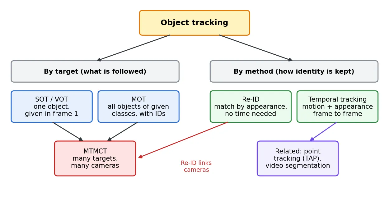
Following [1]:

• By method. Re-identification (Re-ID) matches a target across images that may be far apart in time or come from different cameras, using appearance (and sometimes pose) alone. Temporal object tracking follows targets frame by frame in one video stream, where motion continuity is available.
• By target. Visual object tracking (VOT), also called single-object tracking (SOT), follows one arbitrary object specified by a box in the first frame. Multi-object tracking (MOT) follows all objects of given classes (for example, every pedestrian) through consecutive frames and maintains a consistent ID for each.
• The combined goal. Multi-target multi-camera tracking (MTMCT) tracks many targets across a network of cameras and keeps the same identity when a person leaves one camera’s view and appears in another. It combines MOT within each camera with Re-ID between cameras.

Most of the classical literature, and most benchmarks, use pedestrians as targets [1], because surveillance and autonomous driving made people the most valuable class to track. Modern benchmarks add dancers, athletes, vehicles and open-vocabulary categories.

Person re-identification

Plain version. Re-ID is a search problem: given a photo of a person from one camera, find the same person in photos taken by other cameras, ranked from most to least likely.

Problem formulation

Re-ID is posed as retrieval [7]. A query image $q$ and a gallery $\mathcal{G} = \{g_1, \dots, g_M\}$ of detected person crops from other cameras are mapped by a network $f_\theta$ to embeddings. The gallery is ranked by a distance, usually cosine distance

$$d(q, g) = 1 - \frac{f_\theta(q)^\top f_\theta(g)}{\lVert f_\theta(q)\rVert\,\lVert f_\theta(g)\rVert},$$

where $f_\theta(\cdot) \in \mathbb{R}^D$ is the $D$-dimensional embedding produced by the network with parameters $\theta$. Training makes embeddings of the same identity close and of different identities far apart. A typical recipe combines an identity classification loss (cross-entropy over the $C$ training identities) with a triplet loss

$$\mathcal{L}_{\text{tri}} = \big[\, d(a, p) - d(a, n) + m \,\big]_+ ,$$

where $a$ is an anchor image, $p$ a positive (same identity), $n$ a negative (different identity), $m > 0$ a margin and $[x]_+ = \max(x, 0)$. Test identities never appear in training, so Re-ID is an open-set problem: the network must learn a general notion of “same person”.

Challenges

[1] groups the difficulties into data factors and environment factors. Data factors: limited labeled identities, noisy boxes from the detector, partial bodies, low resolution. Environment factors: different viewpoints and camera color responses, lighting, occlusion, background clutter, and people who change clothes. Re-ID also raises clear privacy concerns, which is part of why surveillance-style datasets have been withdrawn (below). The original post names city-scale surveillance systems as the main application; today Re-ID is just as common as the appearance module inside MOT trackers and in retail and sports analytics.

Representative models

• Strong baselines. Luo et al. [14] showed that a plain ResNet-50 with a set of training “tricks” — warm-up learning rate, random erasing augmentation, label smoothing, last-stride 1 for a larger feature map, and a BNNeck (a batch-norm layer that separates the triplet-loss feature from the classification feature) — is a strong, reproducible baseline.
• Centroid triplet loss (CTL). The model the original post cites (ResNet-50 at $256 \times 128$ input) [15] replaces instance-to-instance triplets with distances to class centroids, and at retrieval time compares a query to identity centroids rather than to every gallery image.
• CLIP-ReID. Li et al. [16] adapt the vision-language model CLIP to Re-ID, where no text labels exist. In a first stage they learn identity-specific text tokens with the encoders frozen; in a second stage they fine-tune the image encoder using those text features as extra supervision.

Datasets

Dataset	Content	Status
Market-1501 [12]	1,501 identities, 6 cameras, detector-cropped boxes	available
MSMT17 [13]	4,101 identities, 15 indoor and outdoor cameras	available
DukeMTMC [10] (and DukeMTMC-reID)	8 synchronized campus cameras	withdrawn in 2019

DukeMTMC was introduced with the IDF1 metric for multi-camera tracking [10], and a Re-ID subset was widely used. Its creators withdrew it in 2019 after privacy and ethics concerns about recording people on a campus, and it should no longer be downloaded or used; Peng et al. [11] trace how derived copies kept circulating afterwards and argue for better dataset stewardship.

Metrics: CMC rank-$k$ and mAP

The cumulative matching characteristic at rank $k$ is the fraction of queries whose first correct match appears in the top $k$ of the ranked gallery:

$$\text{CMC}(k) = \frac{1}{|Q|} \sum_{q \in Q} \mathbb{1}\big[\, r_q \le k \,\big],$$

where $Q$ is the set of queries and $r_q$ is the rank of the first true match for query $q$. Rank-1 accuracy is $\text{CMC}(1)$. Because a query usually has several true matches in the gallery, rank-$k$ alone ignores how well the others are ranked. Mean average precision fixes this:

$$\text{AP}(q) = \frac{1}{G_q}\sum_{i=1}^{G_q} \frac{i}{r_{q,i}}, \qquad \text{mAP} = \frac{1}{|Q|}\sum_{q} \text{AP}(q),$$

where $G_q$ is the number of true matches of $q$ in the gallery and $r_{q,i}$ is the rank of the $i$-th one. So $i / r_{q,i}$ is the precision at the moment the $i$-th true match is found.

import numpy as np

def cmc_map(dist, q_ids, g_ids, max_rank=5):
    """dist: (Q, G) distances between query and gallery embeddings."""
    order = np.argsort(dist, axis=1)                 # closest gallery items first
    match = g_ids[order] == q_ids[:, None]           # (Q, G) True where same person
    cmc = (np.cumsum(match, axis=1) > 0).mean(axis=0)[:max_rank]
    aps = []
    for row in match:
        hits = np.flatnonzero(row)                   # ranks (0-based) of true matches
        precision_at_hits = np.arange(1, len(hits) + 1) / (hits + 1)
        aps.append(precision_at_hits.mean())
    return cmc, np.mean(aps)

rng = np.random.default_rng(0)
centres = rng.normal(size=(50, 64))                  # 50 identities, 64-D embeddings
g_ids = np.repeat(np.arange(50), 4)                  # 4 gallery images per identity
q_ids = np.arange(50)
gallery = centres[g_ids] + 1.6 * rng.normal(size=(200, 64))
query = centres[q_ids] + 1.6 * rng.normal(size=(50, 64))
norm = lambda x: x / np.linalg.norm(x, axis=1, keepdims=True)
dist = 1 - norm(query) @ norm(gallery).T             # cosine distance
cmc, mAP = cmc_map(dist, q_ids, g_ids)
print("rank-1 %.2f  rank-5 %.2f  mAP %.2f" % (cmc[0], cmc[4], mAP))

On this synthetic gallery (4 images per identity) the script prints rank-1 0.76 rank-5 0.92 mAP 0.57: most queries find one correct image near the top, but the other three are scattered, which only mAP reveals.

Single-object tracking

Plain version. You draw a box around something in the first frame; the tracker must keep a box on that same thing for the rest of the video, without knowing in advance what kind of object it is.

Problem formulation

Given frames $I_1, \dots, I_T$ and an initial box $b_1$, a single-object tracker outputs $\hat b_2, \dots, \hat b_T$. The target is class-agnostic: it could be a person, a bird or a coffee cup. This makes SOT a form of one-shot learning: the only example of the target is the first-frame patch, the template $z$. In each new frame the tracker searches a region $x$ around the last position. The challenges [1] lists are complex appearance changes, unusual motion patterns, and environmental change such as lighting and occlusion.

Classical: correlation filters

Before deep learning, the fastest trackers learned a correlation filter online. MOSSE [17] learns a filter $H$ in the Fourier domain so that correlating it with training patches $F_i$ produces sharp Gaussian peaks $G_i$ at the target center:

$$\min_{H^*} \sum_i \big\lvert F_i \odot H^* - G_i \big\rvert^2 \quad\Rightarrow\quad H^* = \frac{\sum_i G_i \odot F_i^*}{\sum_i F_i \odot F_i^*},$$

where capital letters are 2-D discrete Fourier transforms, $\odot$ is element-wise multiplication, $^*$ is complex conjugation and the division is element-wise. Because correlation becomes multiplication in the frequency domain (see DIP Chapter 4), training and detection cost only a few FFTs, so these trackers run at hundreds of frames per second on a CPU. KCF [18] showed that training on all cyclic shifts of a patch gives a circulant data matrix that the DFT diagonalizes, which turns kernel ridge regression into element-wise operations and allows multi-channel features such as HOG. Their weaknesses are a fixed search window, boundary effects from the cyclic assumption, and hand-crafted features.

Siamese trackers

Plain version. Train one network to answer a single question — “where in this search image does the template appear?” — on huge amounts of video offline, then use it frozen at test time.

SiamFC [19] applies the same fully convolutional network $\varphi$ to the template $z$ and the search region $x$ and cross-correlates the two feature maps:

$$f(z, x) = \varphi(z) \star \varphi(x) + b\,\mathbb{1},$$

where $\star$ is cross-correlation (the template features act as a convolution kernel), $b$ is a learned bias and $\mathbb{1}$ is a map of ones. The output is a score map whose peak gives the new position. It is trained with a logistic loss on score-map positions labeled positive near the true center and negative elsewhere. Because nothing is updated online, it is fast and robust to drift, but it only predicts position, with scale handled by searching a small pyramid.

SiamRPN [20] adds a region proposal network after the Siamese features: one branch classifies anchors as target or background, another regresses box offsets. Tracking becomes “one-shot detection” with the template as the class definition, which yields accurate boxes with changing aspect ratios.

Transformer one-stream trackers

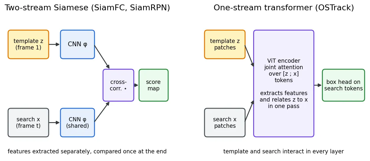
From 2022 the mainstream moved from Siamese CNNs to transformers. The key change is where the template and the search region interact (Figure 2). In a two-stream design they are encoded separately and compared once. In a one-stream design such as OSTrack [21], the image patches of $z$ and $x$ are concatenated into one token sequence and processed by a single Vision Transformer, so that every attention layer both extracts features and relates template to search. OSTrack also drops search tokens that are clearly background in early layers to save computation. SeqTrack [22] goes further in simplicity: an encoder-decoder transformer generates the four box coordinates as a sequence of discrete tokens, autoregressively, trained with plain cross-entropy — the same recipe as language modeling.

Tracking with video segmentation models

Plain version. New “segment anything in video” models can be told “this object” with one click, and then follow it for the whole video as a pixel mask. That is single-object tracking, with a mask instead of a box.

SAM 2 [23] extends the Segment Anything model to video with a streaming memory: features and predicted masks from past frames, plus the prompted frames, are stored in a memory bank that the current frame attends to. Prompting one frame with a click, box or mask yields a “masklet” through the whole video, so it behaves like a mask-output SOT tracker. SAMURAI [24] adapts SAM 2 for tracking without any retraining: it adds a Kalman-filter motion model to choose among SAM 2’s candidate masks and a motion-aware rule for which past frames enter memory, which helps in crowded scenes with similar distractors. SAM 3 [25] adds promptable concept segmentation: given a short noun phrase such as “yellow school bus” or an image exemplar, it detects, segments and tracks all matching instances in a video and gives each its own identity. That is a form of open-vocabulary MOT, and it blurs the old SOT/MOT boundary.

Benchmarks and metrics

Benchmark	What makes it distinct
OTB [26]	early standard benchmark with per-sequence attribute labels (occlusion, fast motion, …); introduced the success and precision plots
VOT challenge [53]	yearly challenge series since 2013, with reset-based protocols; now VOTS, tracking and segmentation
LaSOT [27]	long-term: 1,400 sequences, more than 3.5 million frames, each frame manually annotated
GOT-10k [28]	one-shot protocol: training and test object classes do not overlap
TrackingNet [29]	large-scale, in-the-wild videos with a held-out evaluation server

The two classic measures, from OTB [26], are:

$$\text{Success}(\tau) = \frac{1}{T}\sum_{t=1}^{T} \mathbb{1}\big[\operatorname{IoU}(\hat b_t, b_t) > \tau\big], \qquad \text{AUC} = \int_0^1 \text{Success}(\tau)\, d\tau,$$ $$\text{Precision}(\delta) = \frac{1}{T}\sum_{t=1}^{T} \mathbb{1}\big[\lVert \hat c_t - c_t \rVert_2 \le \delta\big],$$

where $\hat b_t, b_t$ are the predicted and ground-truth boxes, $\tau$ is an IoU threshold, $\hat c_t, c_t$ are their centers and $\delta$ is a pixel distance, conventionally 20. The AUC of the success plot is the headline number on OTB and LaSOT. GOT-10k reports average overlap (the mean IoU) and success rates at $\tau = 0.5$ and $0.75$.

import numpy as np

def iou_xywh(a, b):
    """IoU between rows of a and b, boxes as [x, y, w, h] (top-left corner)."""
    x1 = np.maximum(a[:, 0], b[:, 0]); y1 = np.maximum(a[:, 1], b[:, 1])
    x2 = np.minimum(a[:, 0] + a[:, 2], b[:, 0] + b[:, 2])
    y2 = np.minimum(a[:, 1] + a[:, 3], b[:, 1] + b[:, 3])
    inter = np.clip(x2 - x1, 0, None) * np.clip(y2 - y1, 0, None)
    return inter / (a[:, 2] * a[:, 3] + b[:, 2] * b[:, 3] - inter)

def success_auc(pred, gt, thresholds=np.linspace(0, 1, 21)):
    ious = iou_xywh(pred, gt)
    curve = np.array([(ious > t).mean() for t in thresholds])
    return curve.mean()                              # area under the success plot

def precision_at(pred, gt, px=20):
    c_pred = pred[:, :2] + pred[:, 2:] / 2; c_gt = gt[:, :2] + gt[:, 2:] / 2
    return (np.linalg.norm(c_pred - c_gt, axis=1) <= px).mean()

rng = np.random.default_rng(0)
gt = np.c_[np.linspace(50, 400, 300), np.full(300, 80.0), np.full(300, 40.0), np.full(300, 60.0)]
pred = gt + rng.normal(0, 4, gt.shape)
pred[200:230, :2] += 120                             # 30 frames lost on a distractor
print("success AUC %.3f   precision@20px %.3f" % (success_auc(pred, gt), precision_at(pred, gt)))

This prints success AUC 0.647 precision@20px 0.900: the 30 frames spent on a distractor cost precision 10 points, while the small jitter on the other frames costs AUC much more, because AUC also rewards tight boxes.

Multi-object tracking

Plain version. Find every object of interest in every frame, and give each one a number that stays the same for as long as it is in view — even when objects cross, hide behind each other, or leave and come back.

MOT tracks multiple targets across consecutive frames and maintains a consistent ID for each; a single frame on its own only supports detection. The challenges [1] lists are frequent occlusion, deciding when trajectories start and end, similar appearance between targets, and interaction between targets (people in a crowd move together and occlude each other).

Formally, given detections $\mathcal{D}_t$ in each frame, MOT seeks a set of trajectories $\mathcal{T} = \{\tau_k\}$ that partitions the true detections, discards false positives, and fills in missed ones. Offline methods solve this over the whole video, often as a graph or network-flow problem; online methods, which this section focuses on, must decide at frame $t$ using only frames $1..t$, which is what real-time applications require.

The tracking-by-detection pipeline

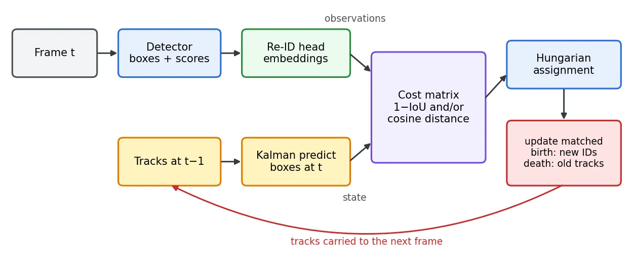
The dominant design for a decade has been tracking-by-detection [2], [4]: run a detector on every frame, then link detections over time (Figure 3). Each frame goes through four steps:

1. Detect. A detector (Faster R-CNN, YOLO-family, DETR-family; see DL 03) gives boxes and scores.
2. Predict. A motion model moves every existing track forward to where it should be now.
3. Describe. Optionally, a Re-ID network embeds each detection crop.
4. Associate. Build a cost matrix between predicted tracks and detections and solve the assignment problem. Matched tracks are updated; unmatched detections may start new tracks (birth); tracks unmatched for too long are deleted (death).

Motion model: the Kalman filter

Plain version. Guess where the object is now from where it was and how fast it was moving; then nudge that guess toward the detection, trusting whichever of the two is less uncertain.

Nearly all tracking-by-detection systems use a linear Kalman filter [30] with a constant-velocity model. In our code the state of one track is

$$\mathbf{x} = [\,c_x,\ c_y,\ w,\ h,\ v_x,\ v_y\,]^\top,$$

where $(c_x, c_y)$ is the box center, $w, h$ its width and height, and $(v_x, v_y)$ the center velocity in pixels per frame. (SORT uses the center, area and aspect ratio instead of $w, h$ [32]; BoT-SORT returns to $w$ and $h$ [36].) The model has two steps.

Predict (time update):

$$\begin{aligned} \hat{\mathbf{x}}_{t \mid t-1} &= \mathbf{F}\,\hat{\mathbf{x}}_{t-1 \mid t-1}, \\ \mathbf{P}_{t \mid t-1} &= \mathbf{F}\,\mathbf{P}_{t-1 \mid t-1}\,\mathbf{F}^\top + \mathbf{Q}, \end{aligned}$$

where $\mathbf{F}$ is the $6\times 6$ transition matrix (identity plus $1$s that add $v_x, v_y$ to $c_x, c_y$, since $\Delta t = 1$ frame), $\mathbf{P}$ is the state covariance (our uncertainty) and $\mathbf{Q}$ is the process noise covariance (how much the true motion can deviate from constant velocity).

Update (measurement update) with a matched detection $\mathbf{z}_t = [c_x, c_y, w, h]^\top$:

$$\begin{aligned} \mathbf{S}_t &= \mathbf{H}\,\mathbf{P}_{t\mid t-1}\,\mathbf{H}^\top + \mathbf{R}, \qquad \mathbf{K}_t = \mathbf{P}_{t\mid t-1}\,\mathbf{H}^\top\,\mathbf{S}_t^{-1}, \\ \hat{\mathbf{x}}_{t\mid t} &= \hat{\mathbf{x}}_{t\mid t-1} + \mathbf{K}_t\big(\mathbf{z}_t - \mathbf{H}\,\hat{\mathbf{x}}_{t\mid t-1}\big), \qquad \mathbf{P}_{t\mid t} = (\mathbf{I} - \mathbf{K}_t\mathbf{H})\,\mathbf{P}_{t\mid t-1}, \end{aligned}$$

where $\mathbf{H} = [\,\mathbf{I}_4\ \ \mathbf{0}\,]$ picks the observed part of the state, $\mathbf{R}$ is the detector’s measurement noise covariance, $\mathbf{z}_t - \mathbf{H}\hat{\mathbf{x}}_{t\mid t-1}$ is the innovation (surprise), $\mathbf{S}_t$ its covariance, and $\mathbf{K}_t$ the Kalman gain. If the prediction is very uncertain ($\mathbf{P}$ large), the update moves the estimate almost all the way to the detection; if the detector is noisy ($\mathbf{R}$ large), it trusts the prediction. When a detection is missing, the tracker runs only the predict step (“coasting”), and $\mathbf{P}$ grows (Figure 4).

import numpy as np
from scipy.optimize import linear_sum_assignment

# ---------- 1. constant-velocity Kalman filter ----------
class KalmanBox:
    """State x = [cx, cy, w, h, vx, vy]; measurement z = [cx, cy, w, h]."""
    def __init__(self, z, q=1.0, r=4.0):
        self.x = np.r_[z, 0.0, 0.0]
        self.P = np.diag([r, r, r, r, 100.0, 100.0])    # unknown velocity: large variance
        self.F = np.eye(6); self.F[0, 4] = self.F[1, 5] = 1.0   # dt = 1 frame
        self.H = np.eye(4, 6)
        self.Q = q * np.diag([1, 1, 0.1, 0.1, 0.5, 0.5])
        self.R = r * np.eye(4)

    def predict(self):
        self.x = self.F @ self.x
        self.P = self.F @ self.P @ self.F.T + self.Q
        return self.x[:4]

    def update(self, z):
        S = self.H @ self.P @ self.H.T + self.R          # innovation covariance
        K = self.P @ self.H.T @ np.linalg.inv(S)          # Kalman gain
        self.x = self.x + K @ (z - self.H @ self.x)
        self.P = (np.eye(6) - K @ self.H) @ self.P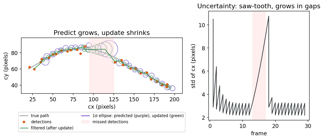

The squared Mahalanobis distance $d_M^2 = \boldsymbol\nu^\top \mathbf{S}^{-1}\boldsymbol\nu$ of an innovation $\boldsymbol\nu$ follows a $\chi^2$ distribution with 4 degrees of freedom under the model, so DeepSORT [33] uses it to gate (forbid) implausible matches. The constant-velocity assumption is also the main weakness: dancers, athletes and anything filmed by a moving camera violate it.

Appearance embeddings

A Re-ID network (previous section) turns each detection crop into a unit vector $\mathbf{e}_j$. Each track keeps an appearance memory, for example an exponential moving average $\mathbf{m}_k \leftarrow \alpha\,\mathbf{m}_k + (1-\alpha)\,\mathbf{e}_j$ followed by renormalization, with $\alpha \in [0, 1)$ (we use $0.9$). The appearance cost is the cosine distance $1 - \mathbf{m}_k^\top \mathbf{e}_j$. Appearance is what lets a tracker recover an identity after a long occlusion, when motion prediction has become useless.

Association: cost matrices and the Hungarian algorithm

Plain version. Make a table of “how bad would it be to match track $k$ with detection $j$” for every pair, then choose the one-to-one matching with the smallest total badness.

With $K$ predicted tracks and $N$ detections, build a cost matrix $\mathbf{C} \in \mathbb{R}^{K \times N}$, for example

$$C_{kj} = \lambda\,\big(1 - \operatorname{IoU}(\hat b_k, b_j)\big) + (1 - \lambda)\,\big(1 - \mathbf{m}_k^\top \mathbf{e}_j\big),$$

where $\hat b_k$ is the predicted box of track $k$, $b_j$ detection $j$‘s box and $\lambda \in [0, 1]$ the weight of motion versus appearance ($\lambda = 1$ is pure IoU, as in SORT). Then solve the linear assignment problem

$$\min_{\mathbf{X} \in \{0,1\}^{K \times N}} \sum_{k,j} C_{kj} X_{kj} \quad \text{s.t.}\quad \sum_j X_{kj} \le 1,\ \ \sum_k X_{kj} \le 1,$$

so each track takes at most one detection and vice versa. The Hungarian algorithm [31] solves it exactly in polynomial time ($O(n^3)$ for $n = \max(K, N)$); SciPy’s linear_sum_assignment implements a fast variant. Finally, any matched pair whose cost exceeds a threshold is rejected, which is how gating is applied in practice.

# ---------- 2. IoU and Hungarian association ----------
def iou_matrix(a, b):
    """a: (N,4), b: (M,4) boxes as [cx, cy, w, h] -> (N,M) IoU."""
    a1, a2 = a[:, None, :2] - a[:, None, 2:] / 2, a[:, None, :2] + a[:, None, 2:] / 2
    b1, b2 = b[None, :, :2] - b[None, :, 2:] / 2, b[None, :, :2] + b[None, :, 2:] / 2
    wh = np.clip(np.minimum(a2, b2) - np.maximum(a1, b1), 0, None)
    inter = wh[..., 0] * wh[..., 1]
    area = lambda x: x[..., 2] * x[..., 3]
    return inter / (area(a)[:, None] + area(b)[None, :] - inter + 1e-9)

def associate(cost, max_cost):
    """Hungarian assignment; pairs whose cost exceeds max_cost are rejected."""
    if cost.size == 0:
        return [], list(range(cost.shape[0])), list(range(cost.shape[1]))
    rows, cols = linear_sum_assignment(cost)
    pairs = [(r, c) for r, c in zip(rows, cols) if cost[r, c] <= max_cost]
    mr = {r for r, _ in pairs}; mc = {c for _, c in pairs}
    return (pairs, [r for r in range(cost.shape[0]) if r not in mr],
            [c for c in range(cost.shape[1]) if c not in mc])

A complete tracker on a synthetic scene

To see what each idea buys, we generate a scene with five pedestrians over 80 frames, designed to contain the classic failure cases:

• objects 0 and 1 cross, and while they overlap, object 1 (behind) gets only low-confidence detections;
• objects 2 and 3 meet and bounce back (non-linear motion, like dancers), with the rear one also low-confidence during the overlap;
• object 4 walks behind a pole for 8 frames, so its detections are low-confidence there;
• every detection is dropped with 5% probability, and there are occasional low-score false positives.

Each detection also carries a 16-D appearance vector: its object’s fixed unit vector plus noise.

# ---------- 3. synthetic scene ----------
def make_scene(T=80, seed=0):
    rng = np.random.default_rng(seed)
    W, H = 30.0, 70.0
    t = np.arange(T, dtype=float)
    tr = {}
    # pair 1: plain crossing, B is behind A (occluded while they overlap)
    tr[0] = np.c_[80 + 5 * t, np.full(T, 120.0)]
    tr[1] = np.c_[480 - 5 * t, np.full(T, 128.0)]
    # pair 2: they meet and bounce back (non-linear motion, like dancers)
    m = 40
    x2 = np.where(t < m, 120 + 4 * t, 120 + 4 * m - 4 * (t - m))
    x3 = np.where(t < m, 440 - 4 * t, 440 - 4 * m + 4 * (t - m))
    tr[2] = np.c_[x2 + 10, np.full(T, 260.0)]
    tr[3] = np.c_[x3 - 10, np.full(T, 266.0)]
    # walker passing behind a pole (frames 30-37): detections become low-score
    tr[4] = np.c_[60 + 3 * t, 40 + 1.0 * t]
    gt = []                                   # per frame list of (id, box)
    dets = []                                 # per frame list of (box, score, gt_id)
    feats = {k: (lambda v: v / np.linalg.norm(v))(rng.normal(size=16)) for k in tr}
    for f in range(T):
        g, d = [], []
        boxes = {k: np.r_[tr[k][f], W, H] for k in tr}
        for k, b in boxes.items():
            g.append((k, b))
            score = rng.uniform(0.6, 0.95)
            if k == 1 and iou_matrix(b[None], boxes[0][None])[0, 0] > 0.2:
                score = rng.uniform(0.15, 0.45)       # occluded by object 0
            if k == 3 and iou_matrix(b[None], boxes[2][None])[0, 0] > 0.2:
                score = rng.uniform(0.15, 0.45)       # occluded by object 2
            if k == 4 and 30 <= f <= 37:
                score = rng.uniform(0.15, 0.45)       # behind the pole
            if rng.random() < 0.05:
                continue                               # random missed detection
            noisy = b + np.r_[rng.normal(0, 2.0, 2), rng.normal(0, 1.0, 2)]
            e = feats[k] + 0.15 * rng.normal(size=16)
            d.append((noisy, score, k, e / np.linalg.norm(e)))
        if rng.random() < 0.3:                         # low-score false positive
            fp = np.r_[rng.uniform(50, 550), rng.uniform(50, 320), W, H]
            e = rng.normal(size=16)
            d.append((fp, rng.uniform(0.1, 0.4), -1, e / np.linalg.norm(e)))
        gt.append(g); dets.append(d)
    return gt, dets

The tracker below has three switches. With both off it is SORT-style: Kalman prediction, IoU cost, Hungarian matching on high-score detections (score $\ge 0.5$), tracks deleted after 2 missed frames. use_low=True adds a BYTE-style second pass: tracks left unmatched try the low-score detections, with IoU only. use_app=True adds the appearance cost to the first pass and a third pass that re-identifies tracks lost for up to 30 frames by appearance alone.

# ---------- 4. SORT-style tracker with optional BYTE and appearance ----------
class Track:
    def __init__(self, tid, z, emb):
        self.id, self.kf, self.emb = tid, KalmanBox(z), emb
        self.lost = 0

def run_tracker(dets, use_low=False, use_app=False, hi=0.5, max_age=2,
                app_age=30, lam=0.5):
    tracks, out, next_id = [], [], 0
    for d in dets:
        for tk in tracks:
            tk.kf.predict()
        boxes = np.array([x[0] for x in d]).reshape(-1, 4)
        scores = np.array([x[1] for x in d])
        embs = np.array([x[3] for x in d]).reshape(-1, 16)
        high = np.where(scores >= hi)[0]
        low = np.where((scores < hi) & (scores >= 0.1))[0]
        active = [tk for tk in tracks if tk.lost <= max_age]
        pred = np.array([tk.kf.x[:4] for tk in active]).reshape(-1, 4)
        # stage 1: high-score detections vs active tracks
        cost = 1 - iou_matrix(pred, boxes[high])
        gate = 0.7
        if use_app and len(active) and len(high):
            tE = np.array([tk.emb for tk in active])
            app = 1 - tE @ embs[high].T            # cosine distance
            cost = np.where(cost > 0.9, 9.0, lam * cost + (1 - lam) * app)
            gate = 0.6
        pairs, ut, ud = associate(cost, gate)
        matched = [(active[r], high[c]) for r, c in pairs]
        rest_tracks = [active[r] for r in ut]
        rest_high = [high[c] for c in ud]
        # stage 2 (BYTE): remaining tracks vs low-score detections, IoU only
        if use_low and rest_tracks and len(low):
            p2 = np.array([tk.kf.x[:4] for tk in rest_tracks])
            pairs2, ut2, _ = associate(1 - iou_matrix(p2, boxes[low]), 0.5)
            matched += [(rest_tracks[r], low[c]) for r, c in pairs2]
            rest_tracks = [rest_tracks[r] for r in ut2]
        # stage 3 (appearance only): long-lost tracks vs leftover high-score dets
        if use_app and rest_high:
            lost = [tk for tk in tracks if max_age < tk.lost <= app_age]
            if lost:
                app = 1 - np.array([tk.emb for tk in lost]) @ embs[rest_high].T
                pairs3, _, ud3 = associate(app, 0.3)
                matched += [(lost[r], rest_high[c]) for r, c in pairs3]
                rest_high = [rest_high[c] for c in ud3]
        for tk, j in matched:
            tk.kf.update(boxes[j]); tk.lost = 0
            tk.emb = 0.9 * tk.emb + 0.1 * embs[j]; tk.emb /= np.linalg.norm(tk.emb)
        hit = {id(tk) for tk, _ in matched}
        for tk in tracks:
            if id(tk) not in hit:
                tk.lost += 1
        for j in rest_high:                           # birth: unmatched high-score
            tracks.append(Track(next_id, boxes[j], embs[j])); next_id += 1
        tracks = [tk for tk in tracks if tk.lost <= (app_age if use_app else max_age)]
        out.append([(tk.id, tk.kf.x[:4].copy()) for tk in tracks if tk.lost == 0])
    return out

The metric code (MOTA, IDF1 and HOTA, explained below) and the experiment:

# ---------- 5. metrics: MOTA, IDF1, HOTA ----------
def frame_match(g, p, thr):
    if not g or not p:
        return []
    iou = iou_matrix(np.array([b for _, b in g]), np.array([b for _, b in p]))
    r, c = linear_sum_assignment(-iou)
    return [(g[i][0], p[j][0]) for i, j in zip(r, c) if iou[i, j] >= thr]

def mota(gt, hyp, thr=0.5):
    fn = fp = idsw = 0; ngt = 0; last = {}
    for g, p in zip(gt, hyp):
        m = frame_match(g, p, thr)
        ngt += len(g); fn += len(g) - len(m); fp += len(p) - len(m)
        for gi, pi in m:
            if gi in last and last[gi] != pi:
                idsw += 1
            last[gi] = pi
    return 1 - (fn + fp + idsw) / ngt, idsw

def idf1(gt, hyp, thr=0.5):
    gids = sorted({i for g in gt for i, _ in g}); pids = sorted({i for p in hyp for i, _ in p})
    gi = {k: n for n, k in enumerate(gids)}; pi = {k: n for n, k in enumerate(pids)}
    ov = np.zeros((len(gids), len(pids)))
    for g, p in zip(gt, hyp):
        if g and p:
            iou = iou_matrix(np.array([b for _, b in g]), np.array([b for _, b in p]))
            for a in range(len(g)):
                for b in range(len(p)):
                    ov[gi[g[a][0]], pi[p[b][0]]] += iou[a, b] >= thr
    r, c = linear_sum_assignment(-ov)
    idtp = ov[r, c].sum()
    n_gt = sum(len(g) for g in gt); n_p = sum(len(p) for p in hyp)
    return 2 * idtp / (n_gt + n_p)

def hota(gt, hyp, alphas=np.arange(0.05, 0.96, 0.05)):
    res = []
    for a in alphas:
        pairs = []; n_gt = n_p = 0
        for g, p in zip(gt, hyp):
            pairs += frame_match(g, p, a); n_gt += len(g); n_p += len(p)
        tp = len(pairs)
        if tp == 0:
            res.append((0, 0, 0)); continue
        cnt = {}
        for q in pairs:
            cnt[q] = cnt.get(q, 0) + 1
        gcount = {}; pcount = {}
        for g in gt:
            for i, _ in g: gcount[i] = gcount.get(i, 0) + 1
        for p in hyp:
            for i, _ in p: pcount[i] = pcount.get(i, 0) + 1
        ass = sum(cnt[q] / (gcount[q[0]] + pcount[q[1]] - cnt[q]) for q in pairs) / tp
        det = tp / (n_gt + n_p - tp)
        res.append((np.sqrt(det * ass), det, ass))
    return np.array(res).mean(axis=0)   # HOTA, DetA, AssA averaged over alpha

gt, dets = make_scene(seed=3)
for name, kw in [("IoU only", {}), ("+ low-score pass", dict(use_low=True)),
                 ("+ appearance", dict(use_low=True, use_app=True))]:
    hyp = run_tracker(dets, **kw)
    m, sw = mota(gt, hyp)
    print(f"{name:18s} MOTA {m:.2f}  IDF1 {idf1(gt, hyp):.2f}  "
          f"HOTA {hota(gt, hyp)[0]:.2f}  ID switches {sw}")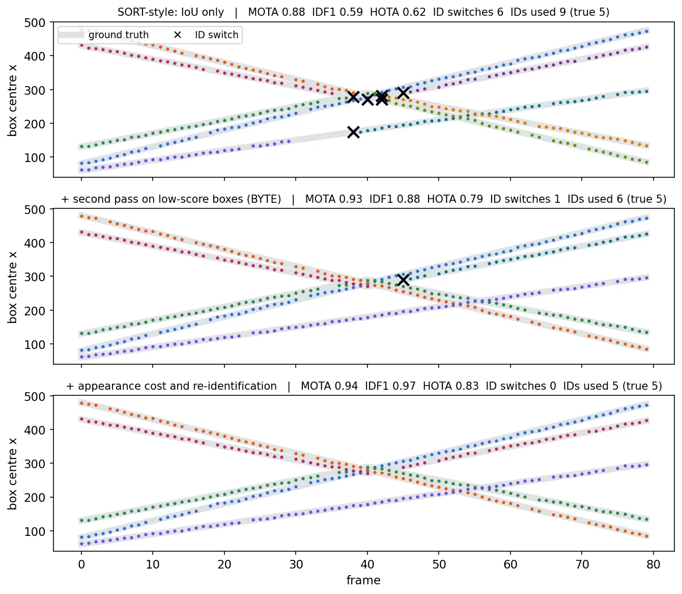

The script prints:

Tracker	MOTA	IDF1	HOTA	ID switches	IDs used (true: 5)
SORT-style, IoU only	0.88	0.59	0.62	6	9
+ BYTE low-score pass	0.93	0.88	0.79	1	6
+ appearance and re-identification	0.94	0.97	0.83	0	5

Read it carefully. The IoU-only tracker loses the occluded objects because their detections fall below the score threshold, so their tracks die and come back with new IDs (fragmentation). The low-score pass keeps them alive, which fixes almost everything, but it cannot fix the bounce: the Kalman filter predicts the two dancers will keep going, so after the overlap one of them is not matched and later restarts with a new ID. Only appearance resolves that. Notice also how little MOTA moves (0.88 → 0.94) compared with IDF1 (0.59 → 0.97): MOTA is mostly a detection measure, a point we return to in the metrics section.

The SORT family

These ideas map directly onto the most cited online trackers:

Tracker	Key idea
SORT [32]	Kalman filter + IoU cost + Hungarian assignment; deliberately minimal and very fast. Showed that detector quality dominates tracking quality.
DeepSORT [33]	Adds a CNN appearance descriptor trained on a person Re-ID dataset, Mahalanobis gating, and a matching cascade that gives priority to recently seen tracks. Fewer ID switches through longer occlusions.
ByteTrack [34]	Associates every detection box: high-score boxes first, then the remaining tracks against low-score boxes using IoU only. Occluded objects often get low scores, so they are recovered instead of discarded, while low-score background boxes stay unmatched and are thrown away.
OC-SORT [35]	“Observation-centric”: when a lost track is re-found, it re-runs the Kalman updates along a virtual trajectory between the last and new observations (fixing error accumulated while coasting), and adds a motion-direction consistency term to the cost. Strong on non-linear motion such as DanceTrack.
BoT-SORT [36]	ByteTrack-style association plus camera-motion compensation (global image registration), a Kalman state with $w, h$ instead of aspect ratio, and a fused IoU/Re-ID cost.

The lesson of this family is that carefully engineered association on top of a strong detector is very hard to beat on pedestrian benchmarks. The 2025 survey of Adžemović [4] reaches the same conclusion: heuristic methods lead on dense scenes with mostly linear motion, while learned association does better when motion is complex.

Joint detection and embedding, and detector-based tracking

Running a separate Re-ID network on every crop is expensive. JDE [37] adds an embedding head to a one-stage detector so that boxes and appearance vectors come out of one forward pass. FairMOT [38] argued that this sharing had been “unfair” to Re-ID: anchor-based detectors produce features that are ambiguous for identity, and detection dominates training. It uses an anchor-free, CenterNet-style detector with two equal branches (detection and Re-ID) on a high-resolution feature map. Tracktor [39], which the original post also cites, removes explicit association for most cases: it feeds the previous frame’s boxes to the detector’s box-regression head, which pulls each box onto the object’s new position and keeps its identity.

Tracking by query: end-to-end MOT

Plain version. Instead of hand-writing “predict, compare, match”, give a transformer a memory slot per object and let it learn to update the slot each frame.

DETR-style detectors (see DL 03) represent objects as queries. MOTR [40] extends this to video: each detected object’s output embedding becomes a track query that is passed to the next frame and keeps predicting the same object, while new detect queries find newborn objects. Identity is carried implicitly by the query; there is no Kalman filter and no Hungarian matching at inference. Training uses a tracklet-aware label assignment and a loss averaged over clips. The weakness was detection quality: one decoder must both detect and associate, and the two tasks conflict. MOTRv2 [41] bootstraps MOTR with proposals from a separate pretrained detector (YOLOX) used as anchors, which eases that conflict. MOTIP [42] (CVPR 2025) reformulates association as ID prediction: given the trajectories so far, each with an ID label drawn from a learnable ID dictionary, a decoder classifies each new detection into one of the existing IDs or “new”. This is in-context, end-to-end trainable, and works with plain object-level features.

Open-vocabulary MOT

Classic MOT only tracks the classes in its training set. OVTrack [43] (CVPR 2023) tracks arbitrary categories by distilling knowledge from a vision-language model (CLIP) for both classification and association, and by learning robust appearance features from hallucinated image pairs produced with a diffusion model. SAM 3’s concept prompts [25] approach the same goal from the segmentation side.

Datasets

Dataset	Domain	What it tests
MOT17 [44]	pedestrians, static and moving cameras	the standard pedestrian benchmark; the MOT16 sequences re-released as MOT17
MOT20 [45]	very crowded pedestrian scenes	heavy occlusion, small targets
DanceTrack [46]	group dancing	uniform appearance and diverse, non-linear motion; appearance cannot separate people
SportsMOT [47]	basketball, volleyball, football (240 sequences)	fast, variable-speed motion with similar but distinguishable appearance
BDD100K MOT [48]	driving video	multi-class tracking (cars, pedestrians, cyclists, …) from a moving vehicle

The shift from MOT17 to DanceTrack and SportsMOT changed the field’s priorities: on MOT17 a good detector and IoU matching go far, but on DanceTrack the motion model and association learning matter most.

Metrics: MOTA, IDF1, HOTA

Plain version. A tracker can fail in two ways: it can miss objects or invent them (detection errors), or it can mix up who is who (association errors). Different metrics weigh these two differently.

All three metrics first match predictions to ground truth in each frame at an IoU threshold. Let $\text{GT}_t$, $\text{FN}_t$, $\text{FP}_t$ and $\text{IDSW}_t$ be the number of ground-truth objects, misses, false positives and identity switches in frame $t$. An identity switch occurs when a ground-truth object is matched to a different predicted ID than at its previous match.

MOTA (CLEAR MOT [9]):

$$\text{MOTA} = 1 - \frac{\sum_t \big(\text{FN}_t + \text{FP}_t + \text{IDSW}_t\big)}{\sum_t \text{GT}_t}.$$

It ranges from $-\infty$ to 1. Because there are usually far more detections than switches, FN and FP dominate it: MOTA is mostly a detection score. A switch is also counted only at the moment it happens, so a tracker that swaps two IDs once and keeps them swapped for 1,000 frames pays the same as one that swaps back after 1 frame.

IDF1 [10] computes a global one-to-one matching between ground-truth trajectories and predicted trajectories (again with the Hungarian algorithm) that maximizes the number of frames where they agree, then

$$\text{IDF1} = \frac{2\,\text{IDTP}}{2\,\text{IDTP} + \text{IDFP} + \text{IDFN}},$$

where IDTP counts detections matched to the trajectory assigned to their ground-truth identity, and IDFP, IDFN the remaining predicted and ground-truth detections. IDF1 measures how long the tracker keeps the right identity, so it is mostly an association score — but because the matching is global, it can behave unintuitively, for example dropping when detection improves.

HOTA (Higher Order Tracking Accuracy [8]) was introduced because neither metric is balanced or decomposable. For a localization threshold $\alpha$, with per-frame matches giving true positives (TP), FN and FP:

$$\text{DetA}_\alpha = \frac{|\text{TP}|}{|\text{TP}| + |\text{FN}| + |\text{FP}|}, \qquad \text{AssA}_\alpha = \frac{1}{|\text{TP}|}\sum_{c \in \text{TP}} \frac{|\text{TPA}(c)|}{|\text{TPA}(c)| + |\text{FNA}(c)| + |\text{FPA}(c)|},$$ $$\text{HOTA}_\alpha = \sqrt{\text{DetA}_\alpha \cdot \text{AssA}_\alpha}, \qquad \text{HOTA} = \frac{1}{19}\sum_{\alpha \in \{0.05,\, 0.10,\, \dots,\, 0.95\}} \text{HOTA}_\alpha .$$

For a matched pair $c$ (ground-truth ID $g$, predicted ID $p$), $\text{TPA}(c)$ is the set of all TPs in the video that also match $g$ to $p$; $\text{FNA}(c)$ the detections of $g$ matched to another ID or missed; $\text{FPA}(c)$ the detections of $p$ matched to another object or to nothing. The geometric mean means a tracker must be good at both detection and association to score well, and DetA and AssA (and a localization accuracy, LocA) can be reported separately to diagnose failures. Averaging over $\alpha$ also rewards precise boxes. (Our code uses a simplified matching that maximizes IoU per frame; the official definition matches with a score that also favors pairs that have been associated before.)

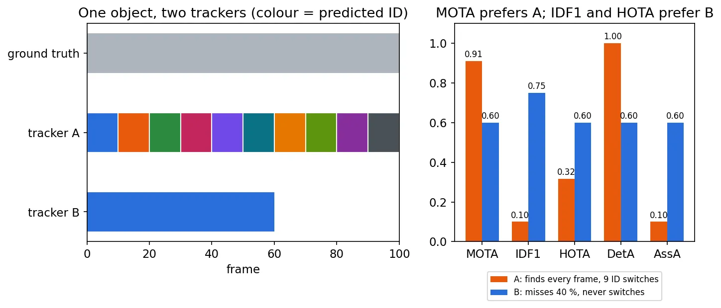
Figure 6 is computed with the functions above: tracker A gets MOTA $= 1 - 9/100 = 0.91$ and AssA $= 0.10$, giving HOTA $= \sqrt{1.0 \times 0.10} \approx 0.32$; tracker B gets $0.60$ on MOTA, DetA, AssA and HOTA, and IDF1 $= 2 \cdot 60 / (100 + 60) = 0.75$. Today, papers on MOT17, MOT20, DanceTrack and SportsMOT report HOTA, IDF1 and MOTA together, and HOTA is usually the primary ranking metric.

Point tracking: a related trend

Plain version. Instead of following whole objects, follow individual points — a freckle on a cheek, a corner of a box — through the whole video, even when they are briefly hidden.

Tracking any point (TAP) asks, for a query point $(x, y)$ in frame $t_0$, for its position and visibility in every other frame. It generalizes optical flow (two frames) to long, occlusion-aware trajectories, and is a natural successor to the classical keypoint tracking from DIP Chapter 12. TAPIR [49] first matches the query feature independently in every frame to get a rough trajectory, then refines it with temporal convolutions. CoTracker [50] tracks many points jointly with a transformer, so points help one another: a point that becomes occluded can be inferred from its visible neighbors. CoTracker3 [51] simplifies the architecture and trains on real videos pseudo-labeled by existing trackers, instead of only synthetic data. Point trackers are now used as motion cues inside object trackers, video editing and robotics.

Multi-target multi-camera tracking

Plain version. Many cameras watch one place. Track everyone in each camera, then figure out that the woman leaving camera 3 is the same woman entering camera 5.

MTMCT is the ultimate goal named in [1]. A typical pipeline runs single-camera MOT to produce tracklets, embeds each tracklet with Re-ID features, and clusters tracklets across cameras using appearance, camera topology (which cameras connect, and travel times between them) and, with calibrated cameras, 3D positions on a ground plane. IDF1 was originally proposed for this setting [10]. The AI City Challenge is the main recurring benchmark. Its ninth edition (2025) [52] made Track 1 a multi-class 3D multi-camera tracking task in warehouse-style environments, with people, humanoid robots, autonomous mobile robots and forklifts, calibrated cameras and 3D box annotations. That shift — from image boxes to calibrated 3D tracks across many views — is where MTMCT is heading.

Modern view

What the surveys say

• Luo et al., “Multiple object tracking: A literature review” [3] (Artificial Intelligence, 2021; first released 2014). The classical reference. It defines the MOT problem formally, categorizes methods by initialization (detection-based versus detection-free), processing mode (online versus offline) and output type (deterministic versus probabilistic), and analyzes the components — appearance model, motion model, interaction model, exclusion constraints, occlusion handling — and the inference methods. Read it to understand the problem independent of any network.
• Ciaparrone et al., “Deep learning in video multi-object tracking: A survey” [2] (Neurocomputing, 2020). Organizes deep MOT around four stages — detection, feature extraction/motion prediction, affinity computation and association — and reviews how deep learning entered each. Its main takeaway, from comparisons on MOTChallenge, is that detection quality and learned appearance features drive most gains.
• Adžemović, “Deep learning-based multi-object tracking: A comprehensive survey from foundations to state-of-the-art” [4] (arXiv, 2025). Splits tracking-by-detection into joint detection-and-embedding, heuristic-based, motion-based, affinity-learning and offline methods, and contrasts them with end-to-end trackers. It identifies 2022 (ByteTrack and MOTR) as the acceleration point and concludes that heuristic trackers lead on crowded, mostly linear scenes while learned association wins on complex motion.
• Marvasti-Zadeh et al., “Deep learning for visual tracking: A comprehensive survey” [5] (IEEE T-ITS, 2022). For SOT. Analyzes deep trackers along nine aspects (network architecture, exploitation, training, objective, output, use of correlation filters, aerial-view, long-term and online tracking) and compares them on OTB, VOT, LaSOT and aerial benchmarks.
• Thangavel (Kugarajeevan) et al., “Transformers in single object tracking: An experimental survey” [6] (IEEE Access, 2023). Classifies transformer trackers as CNN-Transformer hybrids, two-stream two-stage, and one-stream one-stage fully-transformer trackers, and evaluates their robustness and efficiency; the one-stream design (OSTrack-style) emerges as the dominant pattern.
• Ye et al., “Deep learning for person re-identification: A survey and outlook” [7] (IEEE TPAMI, 2022). Separates closed-world Re-ID (feature learning, metric learning, ranking) from open-world Re-ID (heterogeneous data, raw images, noisy labels, unsupervised and open-set settings), proposes the AGW baseline and the mINP metric, which measures the cost of finding all correct matches.
• Luiten et al., “HOTA” [8] (IJCV, 2020). Not a survey, but it re-examines the evaluation of the entire field, shows the biases of MOTA and IDF1 with worked examples and user studies, and is the reason current leaderboards rank by HOTA.

State of the art, 2024–2026

• SOT is dominated by one-stream transformer trackers in the OSTrack/SeqTrack lineage and, increasingly, by segmentation foundation models: SAM 2 with motion-aware memory (SAMURAI) gives strong zero-shot tracking without tracking-specific training [23], [24].
• MOT has two coexisting camps. Heuristic tracking-by-detection (ByteTrack, OC-SORT, BoT-SORT and descendants) remains the default in practice: simple, fast and modular, with a strong detector doing most of the work. End-to-end trackers (MOTR, MOTRv2, MOTIP) lead where motion is complex and appearance is ambiguous, such as DanceTrack and SportsMOT [4], [42].
• Open-vocabulary and promptable tracking is moving into mainstream models: OVTrack established the task, and SAM 3 detects, segments and tracks instances of a text concept with identities [25], [43].
• Point tracking (TAPIR, CoTracker, CoTracker3) matured into a general motion primitive [49]–[51].
• MTMCT is moving to calibrated, multi-class 3D tracking (AI City Challenge 2025) [52].

Open problems

• Long-term occlusion and re-entry. Motion models are useless after a few seconds; appearance must carry identity, but appearance is unreliable for uniform clothing (DanceTrack, sports) and across cameras.
• Non-linear motion and camera motion. Constant-velocity Kalman filters remain the default and are the weak point on dance, sports and driving data; learned motion models are not yet clearly better everywhere.
• End-to-end versus heuristic association. End-to-end trackers are elegant and win on complex motion, but need lots of video training data and compute and still lose to simple heuristics on crowded pedestrian scenes. A unified design that is best on both is open.
• Open-vocabulary and long-tail tracking. Rare classes, and appearance features that generalize to classes never seen in training.
• Evaluation. HOTA fixed much, but benchmarks are pedestrian-heavy, and ID-level evaluation over hours of video and many cameras remains hard. Privacy and dataset ethics (the DukeMTMC lesson) constrain what data can be collected at all.

Key takeaways

• Tracking = detection + time: every tracker must both follow motion and keep identities, and the balance between the two defines SOT, MOT and Re-ID.
• Re-ID is retrieval with learned embeddings; report both CMC rank-$k$ and mAP; DukeMTMC was withdrawn in 2019 and should not be used.
• SOT went from correlation filters (fast, hand-crafted) to Siamese matching (offline-trained) to one-stream transformers; SAM 2-style video segmentation now does SOT with masks, and SAM 3 extends it to many instances from a text prompt.
• Online MOT is a loop of detect → Kalman predict → cost matrix → Hungarian assignment → update/birth/death. Most practical gains come from what goes into the cost matrix and which detections are allowed to match.
• ByteTrack’s low-score pass fixes occlusion fragmentation; appearance fixes non-linear motion and long gaps; end-to-end query trackers learn association directly.
• MOTA mostly measures detection, IDF1 mostly association; HOTA $= \sqrt{\text{DetA}\cdot\text{AssA}}$ (averaged over IoU thresholds) balances and decomposes both.
• The open frontier is long-term identity, non-linear motion, open-vocabulary categories and multi-camera 3D tracking.

Exercises

1. Kalman gain intuition. For a 1-D constant-position model with prior variance $P$ and measurement noise $R$, show that the Kalman gain is $K = P / (P + R)$ and that the posterior variance is $PR/(P+R)$. What happens to $K$ after five frames without detections if each predict step adds $Q$ to $P$?

Hint

With $H = 1$, $S = P + R$ and $K = P/S$. The posterior variance is $(1 - K)P = PR/(P+R)$, smaller than both $P$ and $R$. After five coasting steps the prior is $P + 5Q$, so $K$ moves toward 1: the filter will trust the next detection much more, which is why a wrong match after an occlusion moves the track a lot.

2. Hungarian by hand. Tracks A and B have predicted IoUs with detections 1 and 2 of $\begin{bmatrix} 0.6 & 0.5 \\ 0.55 & 0.0 \end{bmatrix}$. What does greedy matching (highest IoU first) return, and what does the Hungarian algorithm on cost $1 - \text{IoU}$ return? Which total IoU is larger?

Hint

Greedy takes A–1 (0.6) first, leaving B–2 with IoU 0 (rejected), total 0.6. Hungarian picks A–2 and B–1, total $0.5 + 0.55 = 1.05$. Greedy leaves track B unmatched and starts a new ID for detection 2; this is one way ID switches appear.

3. Break the tracker. In the synthetic scene, change the bounce in make_scene so that objects 2 and 3 pass through each other instead (no velocity reversal). Which of the three trackers improves the most, and why?

Hint

With linear motion the constant-velocity prediction is correct through the overlap. With seed=3, the low-score tracker’s IDF1 rises from 0.88 to about 0.96 and it uses the correct 5 IDs, almost matching the appearance tracker (about 0.96 as well); the IoU-only tracker still fragments occluded objects. Appearance helps most exactly when motion is non-linear, which is the design rationale of DanceTrack.

4. Metric arithmetic. A video has one object for 200 frames. A tracker detects it in all frames but uses ID 1 for frames 1–100 and ID 2 for frames 101–200. Compute MOTA, IDF1, DetA, AssA and HOTA at a single threshold, assuming perfect boxes.

Hint

MOTA $= 1 - 1/200 = 0.995$. The best global ID match covers 100 frames: IDF1 $= 2 \cdot 100/(200 + 200) = 0.5$. DetA $= 1$. For each TP, $|\text{TPA}| = 100$, $|\text{FNA}| = 100$, $|\text{FPA}| = 0$, so AssA $= 0.5$ and HOTA $= \sqrt{0.5} \approx 0.71$. One swap barely moves MOTA but halves AssA.

5. Re-ID metrics. In the Re-ID snippet, change the noise level from 1.6 to 2.2 and then to 1.0. How do rank-1 and mAP change, and which one is more sensitive? Explain using the definition of AP.

Hint

mAP falls faster than rank-1 as noise grows, because rank-1 only needs the single easiest true match at the top, while AP penalizes every true match that is pushed down the list. With 4 true matches per query, the hardest one usually decides how much AP is lost.

6. Design question. You must track forklifts and workers across 12 calibrated cameras in a warehouse. Sketch a pipeline using components from this tutorial, and say which metric you would report and why.

Hint

Per-camera detection plus a ByteTrack/BoT-SORT-style tracker; project boxes to the ground plane using calibration; cross-camera association by 3D position and time first, Re-ID appearance second (workers may wear identical vests); handle the two classes separately. Report HOTA (balanced, decomposable into DetA/AssA) and IDF1 (long-term identity across cameras), as in the AI City Challenge setting.

References

1. Shyandram, “物件追蹤Object Tracking 簡介” (Introduction to object tracking), blog post (in Traditional Chinese), 2023; updated 2026. link
2. G. Ciaparrone, F. Luque Sánchez, S. Tabik, L. Troiano, R. Tagliaferri and F. Herrera, “Deep learning in video multi-object tracking: A survey,” Neurocomputing, 2020. arXiv:1907.12740
3. W. Luo, J. Xing, A. Milan, X. Zhang, W. Liu and T.-K. Kim, “Multiple object tracking: A literature review,” Artificial Intelligence, vol. 293, 2021 (arXiv 2014). arXiv:1409.7618
4. M. Adžemović, “Deep learning-based multi-object tracking: A comprehensive survey from foundations to state-of-the-art,” arXiv:2506.13457, 2025. arXiv
5. S. M. Marvasti-Zadeh, L. Cheng, H. Ghanei-Yakhdan and S. Kasaei, “Deep learning for visual tracking: A comprehensive survey,” IEEE Transactions on Intelligent Transportation Systems, vol. 23, 2022. arXiv:1912.00535
6. J. Thangavel (Kugarajeevan), T. Kokul, A. Ramanan and S. Fernando, “Transformers in single object tracking: An experimental survey,” IEEE Access, vol. 11, 2023. arXiv:2302.11867
7. M. Ye, J. Shen, G. Lin, T. Xiang, L. Shao and S. C. H. Hoi, “Deep learning for person re-identification: A survey and outlook,” IEEE TPAMI, vol. 44, 2022. arXiv:2001.04193
8. J. Luiten, A. Ošep, P. Dendorfer, P. Torr, A. Geiger, L. Leal-Taixé and B. Leibe, “HOTA: A higher order metric for evaluating multi-object tracking,” International Journal of Computer Vision, 2020. arXiv:2009.07736
9. K. Bernardin and R. Stiefelhagen, “Evaluating multiple object tracking performance: The CLEAR MOT metrics,” EURASIP Journal on Image and Video Processing, 2008. doi
10. E. Ristani, F. Solera, R. S. Zou, R. Cucchiara and C. Tomasi, “Performance measures and a data set for multi-target, multi-camera tracking,” ECCV Workshop on Benchmarking Multi-Target Tracking, 2016. arXiv:1609.01775
11. K. Peng, A. Mathur and A. Narayanan, “Mitigating dataset harms requires stewardship: Lessons from 1000 papers,” arXiv:2108.02922, 2021. arXiv
12. L. Zheng, L. Shen, L. Tian, S. Wang, J. Wang and Q. Tian, “Scalable person re-identification: A benchmark,” ICCV, 2015. doi
13. L. Wei, S. Zhang, W. Gao and Q. Tian, “Person transfer GAN to bridge domain gap for person re-identification,” CVPR, 2018. arXiv:1711.08565
14. H. Luo, Y. Gu, X. Liao, S. Lai and W. Jiang, “Bag of tricks and a strong baseline for deep person re-identification,” CVPR Workshops, 2019. arXiv:1903.07071
15. M. Wieczorek, B. Rychalska and J. Dąbrowski, “On the unreasonable effectiveness of centroids in image retrieval,” arXiv:2104.13643, 2021. arXiv
16. S. Li, L. Sun and Q. Li, “CLIP-ReID: Exploiting vision-language model for image re-identification without concrete text labels,” AAAI, 2023. arXiv:2211.13977
17. D. S. Bolme, J. R. Beveridge, B. A. Draper and Y. M. Lui, “Visual object tracking using adaptive correlation filters,” CVPR, 2010. doi
18. J. F. Henriques, R. Caseiro, P. Martins and J. Batista, “High-speed tracking with kernelized correlation filters,” IEEE TPAMI, vol. 37, 2015. arXiv:1404.7584
19. L. Bertinetto, J. Valmadre, J. F. Henriques, A. Vedaldi and P. H. S. Torr, “Fully-convolutional Siamese networks for object tracking,” arXiv:1606.09549, 2016 (ECCV 2016 workshops). arXiv
20. B. Li, J. Yan, W. Wu, Z. Zhu and X. Hu, “High performance visual tracking with Siamese region proposal network,” CVPR, 2018. doi
21. B. Ye, H. Chang, B. Ma, S. Shan and X. Chen, “Joint feature learning and relation modeling for tracking: A one-stream framework” (OSTrack), ECCV, 2022. arXiv:2203.11991
22. X. Chen, H. Peng, D. Wang, H. Lu and H. Hu, “SeqTrack: Sequence to sequence learning for visual object tracking,” CVPR, 2023 (the arXiv entry was later extended as SeqTrackv2). arXiv:2304.14394
23. N. Ravi, V. Gabeur, Y.-T. Hu, R. Hu, C. Ryali, T. Ma et al., “SAM 2: Segment anything in images and videos,” ICLR, 2025. arXiv:2408.00714
24. C.-Y. Yang, H.-W. Huang, W. Chai, Z. Jiang and J.-N. Hwang, “SAMURAI: Adapting segment anything model for zero-shot visual tracking with motion-aware memory,” arXiv:2411.11922, 2024. arXiv
25. N. Carion, L. Gustafson, Y.-T. Hu et al., “SAM 3: Segment anything with concepts,” ICLR, 2026. arXiv:2511.16719
26. Y. Wu, J. Lim and M.-H. Yang, “Object tracking benchmark,” IEEE TPAMI, vol. 37, 2015. doi
27. H. Fan, L. Lin, F. Yang, P. Chu, G. Deng, S. Yu et al., “LaSOT: A high-quality benchmark for large-scale single object tracking,” CVPR, 2019. arXiv:1809.07845
28. L. Huang, X. Zhao and K. Huang, “GOT-10k: A large high-diversity benchmark for generic object tracking in the wild,” IEEE TPAMI, vol. 43, 2021. arXiv:1810.11981
29. M. Müller, A. Bibi, S. Giancola, S. Al-Subaihi and B. Ghanem, “TrackingNet: A large-scale dataset and benchmark for object tracking in the wild,” arXiv:1803.10794, 2018 (ECCV 2018). arXiv
30. R. E. Kalman, “A new approach to linear filtering and prediction problems,” Journal of Basic Engineering, vol. 82, no. 1, pp. 35–45, 1960. doi
31. H. W. Kuhn, “The Hungarian method for the assignment problem,” Naval Research Logistics Quarterly, vol. 2, pp. 83–97, 1955. doi
32. A. Bewley, Z. Ge, L. Ott, F. Ramos and B. Upcroft, “Simple online and realtime tracking,” ICIP, 2016. arXiv:1602.00763
33. N. Wojke, A. Bewley and D. Paulus, “Simple online and realtime tracking with a deep association metric,” ICIP, 2017. doi
34. Y. Zhang, P. Sun, Y. Jiang, D. Yu, F. Weng, Z. Yuan, P. Luo, W. Liu and X. Wang, “ByteTrack: Multi-object tracking by associating every detection box,” ECCV, 2022. arXiv:2110.06864
35. J. Cao, J. Pang, X. Weng, R. Khirodkar and K. Kitani, “Observation-centric SORT: Rethinking SORT for robust multi-object tracking,” CVPR, 2023. arXiv:2203.14360
36. N. Aharon, R. Orfaig and B.-Z. Bobrovsky, “BoT-SORT: Robust associations multi-pedestrian tracking,” arXiv:2206.14651, 2022. arXiv
37. Z. Wang, L. Zheng, Y. Liu, Y. Li and S. Wang, “Towards real-time multi-object tracking” (JDE), ECCV, 2020. arXiv:1909.12605
38. Y. Zhang, C. Wang, X. Wang, W. Zeng and W. Liu, “FairMOT: On the fairness of detection and re-identification in multiple object tracking,” IJCV, 2021. arXiv:2004.01888
39. P. Bergmann, T. Meinhardt and L. Leal-Taixé, “Tracking without bells and whistles” (Tracktor), ICCV, 2019. arXiv:1903.05625
40. F. Zeng, B. Dong, Y. Zhang, T. Wang, X. Zhang and Y. Wei, “MOTR: End-to-end multiple-object tracking with transformer,” ECCV, 2022. arXiv:2105.03247
41. Y. Zhang, T. Wang and X. Zhang, “MOTRv2: Bootstrapping end-to-end multi-object tracking by pretrained object detectors,” CVPR, 2023. arXiv:2211.09791
42. R. Gao, J. Qi and L. Wang, “Multiple object tracking as ID prediction” (MOTIP), CVPR, 2025. arXiv:2403.16848
43. S. Li, T. Fischer, L. Ke, H. Ding, M. Danelljan and F. Yu, “OVTrack: Open-vocabulary multiple object tracking,” CVPR, 2023. arXiv:2304.08408
44. A. Milan, L. Leal-Taixé, I. Reid, S. Roth and K. Schindler, “MOT16: A benchmark for multi-object tracking,” arXiv:1603.00831, 2016 (MOT16/MOT17). arXiv
45. P. Dendorfer, H. Rezatofighi, A. Milan, J. Shi, D. Cremers, I. Reid, S. Roth, K. Schindler and L. Leal-Taixé, “MOT20: A benchmark for multi object tracking in crowded scenes,” arXiv:2003.09003, 2020. arXiv
46. P. Sun, J. Cao, Y. Jiang, Z. Yuan, S. Bai, K. Kitani and P. Luo, “DanceTrack: Multi-object tracking in uniform appearance and diverse motion,” CVPR, 2022. arXiv:2111.14690
47. Y. Cui, C. Zeng, X. Zhao, Y. Yang, G. Wu and L. Wang, “SportsMOT: A large multi-object tracking dataset in multiple sports scenes,” ICCV, 2023. arXiv:2304.05170
48. F. Yu, H. Chen, X. Wang, W. Xian, Y. Chen, F. Liu, V. Madhavan and T. Darrell, “BDD100K: A diverse driving dataset for heterogeneous multitask learning,” CVPR, 2020. arXiv:1805.04687
49. C. Doersch, Y. Yang, M. Vecerik, D. Gokay, A. Gupta, Y. Aytar et al., “TAPIR: Tracking any point with per-frame initialization and temporal refinement,” ICCV, 2023. arXiv:2306.08637
50. N. Karaev, I. Rocco, B. Graham, N. Neverova, A. Vedaldi and C. Rupprecht, “CoTracker: It is better to track together,” ECCV, 2024. arXiv:2307.07635
51. N. Karaev, I. Makarov, J. Wang, N. Neverova, A. Vedaldi and C. Rupprecht, “CoTracker3: Simpler and better point tracking by pseudo-labelling real videos,” arXiv:2410.11831, 2024. arXiv
52. Z. Tang, S. Wang, D. C. Anastasiu et al., “The 9th AI City Challenge,” ICCV Workshops, 2025. arXiv:2508.13564
53. VOT Challenge organizers, “The Visual Object Tracking (VOT) challenge series,” website, 2013–present. votchallenge.net