DL 02 · Deep Image Classification

What you’ll learn

• How image classification is posed precisely: single-label, multi-label and fine-grained tasks; logits, softmax and cross-entropy; top-1/top-5 accuracy; and what it means for a classifier to be calibrated.
• What the standard datasets (MNIST, CIFAR, ImageNet, iNaturalist) are for, and what reproduction studies such as ImageNetV2 revealed about benchmark accuracy.
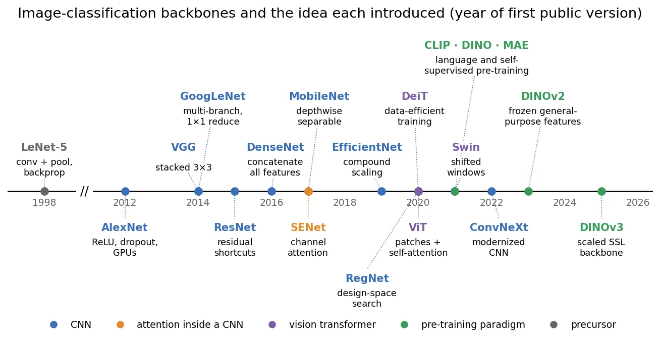
• The design reasoning behind each major backbone, from AlexNet, VGG, Inception and ResNet to MobileNet, EfficientNet, RegNet, ConvNeXt, ViT, DeiT and Swin, with parameter and cost arithmetic you can check yourself.
• Which parts of a modern training recipe matter (augmentation, Mixup/CutMix, label smoothing, AdamW, warmup + cosine, stochastic depth, EMA) and why recipes alone moved ResNet-50 by several points.
• How pre-training changed the job: linear probes and fine-tuning, contrastive and masked self-supervision, DINOv2-style frozen features and CLIP zero-shot classification.
• How to evaluate honestly: distribution shift, adversarial examples, shortcut learning, temperature scaling, efficiency metrics and Grad-CAM.

The big picture

Image classification asks one question of a whole image: which of these labels fits? It is the oldest deep-learning benchmark task and still the place where most backbone networks are born. A detector, a segmenter or a restoration network usually starts from a backbone that was first trained, or at least evaluated, as an image classifier.

This tutorial assumes you know what a convolution, a CNN layer and backpropagation are. The classical side of classification (Bayes classifiers, perceptrons, a small CNN written in NumPy, softmax and cross-entropy derived by hand) is in DIP Chapter 13. The broad history of deep learning for images is in DL 01. Here we go deep on classification itself. For a compact refresher on activation functions and optimizers in Chinese, see the notes 機器學習及類神經網路筆記. A good single survey of the CNN side of this story is Li et al. [1].

The classification problem

Plain version. The network looks at an image and outputs one score per class. We turn scores into probabilities, compare them with the true label, and nudge the network so the right class gets more probability next time.

Single-label, multi-label and fine-grained

Let $\mathbf{x} \in \mathbb{R}^{H \times W \times 3}$ be an RGB image and $\mathcal{Y} = \{1, \dots, K\}$ a set of $K$ classes. A network $f_\theta$ with parameters $\theta$ maps the image to a vector of logits $\mathbf{z} = f_\theta(\mathbf{x}) \in \mathbb{R}^K$, one unnormalized score per class.

• Single-label (multi-class) classification assumes exactly one correct class $y \in \mathcal{Y}$. The logits are turned into a probability vector with the softmax,

$$p_k = \frac{e^{z_k}}{\sum_{j=1}^{K} e^{z_j}}, \qquad k = 1, \dots, K,$$

where $p_k$ is the model’s estimate of $P(y = k \mid \mathbf{x})$. Training minimizes the cross-entropy, the negative log-probability of the true class, averaged over a mini-batch:

$$\mathcal{L}_{\text{CE}} = -\frac{1}{B}\sum_{i=1}^{B} \log p_{y_i}(\mathbf{x}_i),$$

where $B$ is the batch size and $y_i$ the label of image $\mathbf{x}_i$. The gradient with respect to the logits is $\partial \mathcal{L}/\partial \mathbf{z} = \mathbf{p} - \mathbf{e}_y$ (per image), with $\mathbf{e}_y$ the one-hot vector of the true class; DIP Chapter 13 derives it.

• Multi-label classification allows any subset of labels (a street photo can contain “car”, “person” and “bicycle”). Each class gets an independent sigmoid $\sigma(z_k) = 1/(1 + e^{-z_k})$ and a binary cross-entropy, $-\sum_k [t_k \log \sigma(z_k) + (1 - t_k)\log(1 - \sigma(z_k))]$, where $t_k \in \{0, 1\}$ says whether class $k$ is present. Metrics change too: mean average precision over classes replaces accuracy.

• Fine-grained classification separates visually similar subordinate classes, such as 200 bird species or 1,000 aircraft variants. The loss is the same as single-label, but the signal lives in small parts (a beak shape, a wing bar), classes are often long-tailed, and label noise from non-expert annotators is common. iNaturalist [6] is the standard large fine-grained benchmark.

Metrics: top-1, top-5 and beyond

Top-1 accuracy is the fraction of images whose highest-scoring class is the true one. Top-$k$ accuracy counts an image as correct if the true class is among the $k$ highest scores. The ImageNet challenge reported top-5 error because many images contain several objects, and some classes are nearly indistinguishable [2]. Top-5 hides real mistakes, so modern papers mostly report top-1. For imbalanced data, report balanced accuracy (the mean of per-class recalls) or per-class results, because a classifier can score high accuracy by ignoring rare classes.

import torch
import torch.nn.functional as F

logits = torch.tensor([[2.0, 1.0, 0.1, -1.0],    # 2 images, 4 classes
                       [0.5, 2.5, 2.4, 0.0]])
y = torch.tensor([0, 2])

p = logits.softmax(dim=1)
ce = F.cross_entropy(logits, y)                       # mean of -log p[i, y_i]
ce_ls = F.cross_entropy(logits, y, label_smoothing=0.1)
top1 = (logits.argmax(1) == y).float().mean()
top2 = (logits.topk(2, dim=1).indices == y[:, None]).any(1).float().mean()
print(p.round(decimals=3))
print(f"CE {ce:.3f}  CE+LS {ce_ls:.3f}  top-1 {top1:.2f}  top-2 {top2:.2f}")

# multi-label: one independent sigmoid per class, binary cross-entropy
targets = torch.tensor([[1., 0., 1., 0.], [0., 1., 1., 0.]])
print(f"BCE {F.binary_cross_entropy_with_logits(logits, targets):.3f}")

The second image is a near-tie between classes 1 and 2. Top-1 counts it as wrong; top-2 counts it as right. That one example is the whole argument for and against top-5.

Calibration: are the probabilities honest?

Accuracy only checks the argmax. Calibration checks whether the confidence means what it says: among all predictions made with confidence 0.8, about 80% should be right. Formally, a classifier is calibrated if $P(\hat{y} = y \mid \hat{p} = c) = c$ for every confidence $c$, where $\hat{y}$ is the predicted class and $\hat{p} = \max_k p_k$ its probability. The usual summary is the expected calibration error: split predictions into $M$ confidence bins $B_m$ and compute

$$\text{ECE} = \sum_{m=1}^{M} \frac{|B_m|}{n}\,\big|\operatorname{acc}(B_m) - \operatorname{conf}(B_m)\big|,$$

where $n$ is the number of test images, $\operatorname{acc}(B_m)$ the accuracy inside bin $m$ and $\operatorname{conf}(B_m)$ the mean confidence there. Guo et al. [47] found that modern deep networks, trained long with cross-entropy, tend to be overconfident, and that a single scalar fix works remarkably well. We return to it in the robustness section.

Datasets and why they matter

Plain version. A benchmark is a frozen exam. It lets everyone compare methods fairly, but once a whole field studies for the same exam, scores start to measure the exam as much as the skill.

Dataset	Images	Classes	Resolution	Role
MNIST [3]	60k train / 10k test	10 digits	28×28 gray	sanity check, teaching
CIFAR-10 / CIFAR-100 [4]	50k train / 10k test	10 / 100 (20 superclasses)	32×32 RGB	small-scale architecture and recipe studies
ImageNet-1k (ILSVRC 2012) [2]	about 1.28M train / 50k val	1,000	variable, usually trained at 224×224	the standard backbone benchmark
ImageNet-21k [5]	roughly 13–14M (versions differ)	about 21k	variable	larger-scale supervised pre-training
iNaturalist [6]	hundreds of thousands, by year	thousands of species	variable	fine-grained, long-tailed

MNIST is solved and now only catches bugs. CIFAR is small enough to run many controlled experiments, which is why regularization papers love it. ImageNet-1k became the reference after the 2012 challenge [2], [10]: architectures are usually reported as “top-1 on ImageNet-1k val at 224×224”, and almost every pre-trained backbone in a model zoo has an ImageNet number attached. ImageNet-21k is the larger hierarchy from which ImageNet-1k was drawn; Ridnik et al. [5] made pre-training on it practical with a cleaned, semantic-hierarchy-aware recipe.

How reliable are the numbers?

Three lines of work changed how we read ImageNet accuracy.

• Reproduction. Recht et al. [7] rebuilt test sets for CIFAR-10 and ImageNet by repeating the original collection procedure as closely as possible (ImageNetV2). Every model lost accuracy: 3–15% on CIFAR-10 and 11–14% on ImageNet. But the ranking was largely preserved, and gains on the old test set translated into gains on the new one. Their reading is that the drop comes from a subtle shift in difficulty between the old and new samples, not from the community overfitting to the test set by reusing it.
• Labels. Beyer et al. [8] re-annotated the ImageNet validation set with multiple labels per image and found that recent “progress” partly reflects fitting the idiosyncrasies of the original single-label annotations. Northcutt et al. [9] estimated that label errors are pervasive across common test sets and showed that they can change which model looks best.
• Bias. Every dataset has a “signature” in viewpoint, background and photographer style. DIP Chapter 13 reviews the dataset-bias studies; the practical lesson is to test on independently collected data whenever possible.

CNN architectures and the reasons behind them

Plain version. Each famous CNN fixed one specific problem of its predecessors: training too slow, too many parameters, too hard to optimize when deep, too expensive on a phone. Knowing the problem each one solved is more useful than memorizing their layer tables.

AlexNet: depth becomes trainable

Before 2012, the best ImageNet systems used hand-crafted features (SIFT, Fisher vectors) with linear classifiers. AlexNet [10] was a five-convolution, three-fully-connected network trained end to end on ImageNet. Three ingredients made it work at that scale. ReLU activations, $\max(0, z)$, do not saturate for positive inputs, so gradients do not vanish the way they do with tanh, and the paper reports several times faster training. Dropout in the large fully connected layers fought overfitting; those layers held most of the parameters. GPUs made it feasible: the model was split across two GPUs. Heavy data augmentation (random crops and flips, color perturbation) was the fourth, often forgotten, ingredient. The design lesson: with enough data and compute, learned features beat engineered ones.

VGG: small kernels, stacked

VGG [11] asked a cleaner question: what happens if we only use $3 \times 3$ convolutions and go deeper (16–19 weight layers)? Two stacked $3 \times 3$ layers see a $5 \times 5$ region; three see $7 \times 7$. For $C$ input and output channels,

$$\underbrace{2 \cdot 3^2 C^2}_{\text{two } 3\times 3} = 18C^2 \;\lt\; \underbrace{5^2 C^2}_{\text{one } 5\times 5} = 25C^2 ,$$

ignoring biases. So the stack has fewer parameters for the same receptive field, and it inserts an extra nonlinearity between the two layers. VGG’s uniform design made it a favourite feature extractor for years. Its weakness is cost: the fully connected head and the wide early layers make it heavy.

GoogLeNet / Inception: width, branches and $1 \times 1$ bottlenecks

GoogLeNet [12] attacked cost instead. Each Inception module runs $1 \times 1$, $3 \times 3$, $5 \times 5$ convolutions and pooling in parallel and concatenates the outputs, so the next layer can choose the right scale. Running big kernels on many channels would be expensive, so $1 \times 1$ convolutions first reduce the channel count. A $1 \times 1$ convolution is a per-pixel linear map across channels: it mixes channels without looking at neighbours, and it is the cheapest way to change width. GoogLeNet also replaced the large fully connected head with global average pooling. The follow-up Inception-v3 paper [13] factorized large kernels into stacks or into $1 \times n$ and $n \times 1$ pairs, and introduced label smoothing, which we meet again in the training section.

ResNet: learning residuals

The problem. Stacking more plain layers eventually made networks worse, even on the training set. This “degradation” is an optimization problem, not overfitting: a deeper network could in principle copy a shallower one and set the extra layers to identity, yet SGD did not find that solution.

The idea. He et al. [14] let a block learn a residual $\mathcal{F}$ and add its input back:

$$\mathbf{y} = \mathcal{F}(\mathbf{x}; \{W_i\}) + \mathbf{x},$$

where $\mathbf{x}$ is the block input, $\mathcal{F}$ is two or three convolution layers with weights $W_i$, and $\mathbf{y}$ the output. If the best mapping is close to identity, the block only has to push $\mathcal{F}$ toward zero, which is easy. When the shapes differ (more channels, stride 2), the shortcut becomes a $1 \times 1$ projection.

Why it trains. Unroll $L$ blocks of the pre-activation form $\mathbf{x}_{l+1} = \mathbf{x}_l + \mathcal{F}(\mathbf{x}_l)$, as analysed in the follow-up paper on identity mappings [15]:

$$\mathbf{x}_L = \mathbf{x}_l + \sum_{i=l}^{L-1} \mathcal{F}(\mathbf{x}_i), \qquad \frac{\partial \mathcal{L}}{\partial \mathbf{x}_l} = \frac{\partial \mathcal{L}}{\partial \mathbf{x}_L}\Big(\mathbf{I} + \frac{\partial}{\partial \mathbf{x}_l}\sum_{i=l}^{L-1} \mathcal{F}(\mathbf{x}_i)\Big),$$

where $\mathcal{L}$ is the loss and $\mathbf{I}$ the identity matrix. The identity term carries the gradient from the top straight down to any block, so it cannot vanish through a product of many small Jacobians. That paper also found that keeping the shortcut a pure identity (moving BN and ReLU inside the residual branch, “pre-activation”) trains even deeper networks more easily.

The bottleneck. For deeper ResNets (50 layers and up) each block becomes $1 \times 1$ (reduce) → $3 \times 3$ → $1 \times 1$ (expand), shown in Figure 2(c). At 256 channels, a basic block of two $3 \times 3$ convolutions has $2 \cdot 9 \cdot 256^2 \approx 1.18$M weights; a bottleneck that reduces to 64 channels has $256 \cdot 64 + 9 \cdot 64^2 + 64 \cdot 256 \approx 70$k. The expensive $3 \times 3$ runs on a thin tensor, which is what makes 50–152 layers affordable.

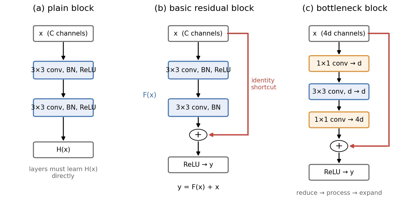
The basic block used in this tutorial’s experiments, written in PyTorch:

import torch.nn as nn
import torch.nn.functional as F

class BasicBlock(nn.Module):
    def __init__(self, cin, cout, stride=1):
        super().__init__()
        self.conv1 = nn.Conv2d(cin, cout, 3, stride, 1, bias=False)
        self.bn1 = nn.BatchNorm2d(cout)
        self.conv2 = nn.Conv2d(cout, cout, 3, 1, 1, bias=False)
        self.bn2 = nn.BatchNorm2d(cout)
        self.short = nn.Identity()
        if stride != 1 or cin != cout:   # projection shortcut when shapes change
            self.short = nn.Sequential(nn.Conv2d(cin, cout, 1, stride, bias=False), nn.BatchNorm2d(cout))

    def forward(self, x):
        out = F.relu(self.bn1(self.conv1(x)))
        out = self.bn2(self.conv2(out))
        return F.relu(out + self.short(x))   # y = F(x) + x

DenseNet: reuse everything

DenseNet [16] pushes feature reuse further: inside a dense block, layer $\ell$ receives the concatenation of all earlier feature maps, $\mathbf{x}_\ell = H_\ell([\mathbf{x}_0, \mathbf{x}_1, \dots, \mathbf{x}_{\ell-1}])$, where $[\cdot]$ is channel concatenation and $H_\ell$ is BN–ReLU–conv. Each layer adds only a few channels (the “growth rate”), so the network is parameter-efficient, and every layer has a short path to the loss. The cost is memory: concatenated activations grow with depth, which made DenseNets slower in practice than their parameter count suggests. A useful lesson for later: parameters, FLOPs and wall-clock time are three different things.

MobileNet: factorize the convolution

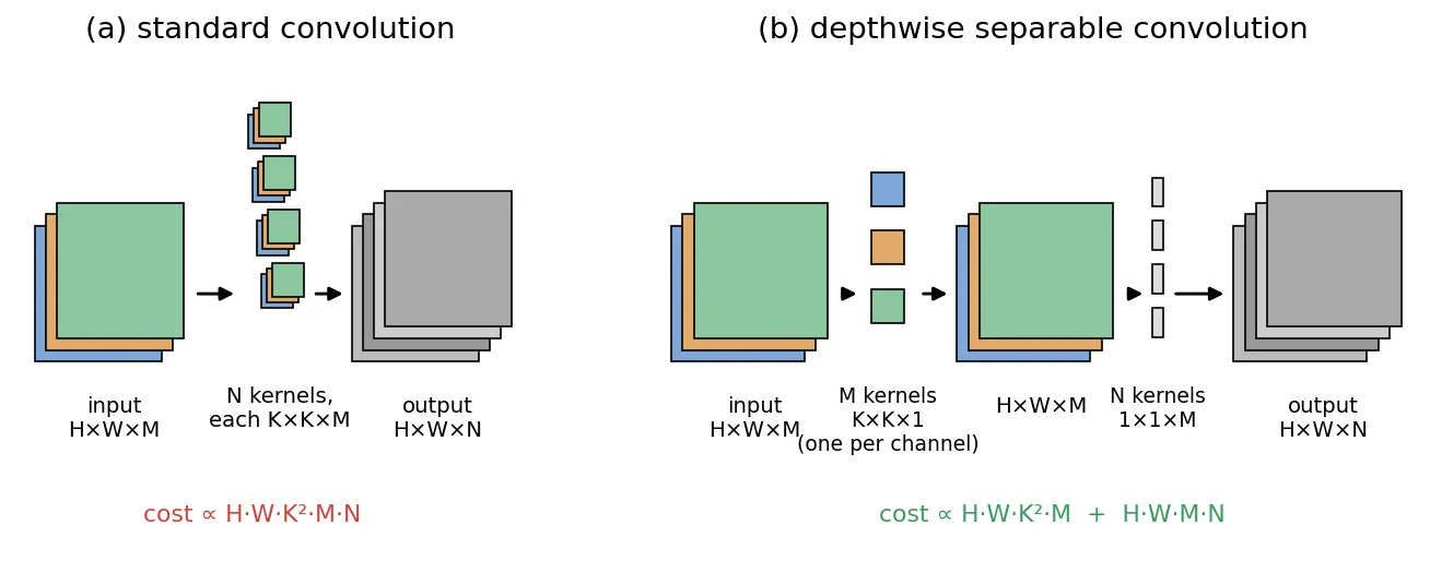
MobileNet [17] targets phones. A standard $K \times K$ convolution from $M$ to $N$ channels on an $H \times W$ map costs $H W K^2 M N$ multiply–adds. A depthwise separable convolution splits it into a depthwise $K \times K$ convolution that filters each channel separately ($H W K^2 M$) and a pointwise $1 \times 1$ convolution that mixes channels ($H W M N$). The cost ratio is

$$\frac{H W K^2 M + H W M N}{H W K^2 M N} = \frac{1}{N} + \frac{1}{K^2},$$

so with $K = 3$ and many output channels the separable version is roughly 8–9 times cheaper. The bet is that spatial filtering and channel mixing do not need to be learned jointly. That bet held up so well that depthwise convolutions reappear in EfficientNet and ConvNeXt.

import torch.nn as nn

def n_params(m):
    return sum(p.numel() for p in m.parameters())

M, N, K = 128, 128, 3
standard = nn.Conv2d(M, N, K, padding=1, bias=False)
separable = nn.Sequential(nn.Conv2d(M, M, K, padding=1, groups=M, bias=False),   # depthwise
                          nn.Conv2d(M, N, 1, bias=False))                          # pointwise
print("standard:", n_params(standard), " separable:", n_params(separable),
      f" ratio {n_params(separable) / n_params(standard):.3f} vs 1/N + 1/K^2 = {1/N + 1/K**2:.3f}")
# standard: 147456  separable: 17536  ratio 0.119 vs 1/N + 1/K^2 = 0.119

EfficientNet: scale depth, width and resolution together

Given a good small network, how should we make it bigger? Deeper, wider, or higher input resolution? Tan and Le [18] argued these interact: a higher resolution image needs more depth (larger receptive field) and more width (finer patterns). Compound scaling grows all three with one coefficient $\phi$:

$$d = \alpha^{\phi}, \quad w = \beta^{\phi}, \quad r = \gamma^{\phi}, \qquad \text{s.t. } \alpha \beta^2 \gamma^2 \approx 2, \;\; \alpha, \beta, \gamma \ge 1,$$

where $d$, $w$, $r$ multiply depth, width and resolution. FLOPs scale roughly as $d\,w^2 r^2$, so each unit increase of $\phi$ roughly doubles the cost. The constants are found by a small grid search on the base network (itself found by architecture search, using inverted-bottleneck blocks with depthwise convolutions and squeeze-and-excitation). The idea, “scale in a balanced way”, outlived the specific constants.

RegNet: design spaces instead of single designs

Radosavovic et al. [19] studied populations of networks rather than single winners. Starting from a broad space of ResNet-like networks, they repeatedly constrained it (for example, shared bottleneck ratios, widths that increase across stages) and checked whether the distribution of errors improved. The surviving space, RegNet, describes stage widths with a simple quantized linear rule. The lesson is methodological: good architectures follow simple regularities, and comparing distributions of models is more reliable than comparing one tuned model against another.

ConvNeXt: a CNN modernized step by step

After vision transformers took over the leaderboards, Liu et al. [20] asked how much of their advantage came from attention and how much from everything else. They started from a ResNet-50 trained with a transformer-style recipe and changed one thing at a time: stage ratios like Swin’s, a “patchify” stem (a $4 \times 4$ stride-4 convolution), depthwise convolutions with larger $7 \times 7$ kernels, an inverted bottleneck, fewer activations and normalizations, GELU and LayerNorm. The result, ConvNeXt, matched Swin-style transformers of similar cost on ImageNet and downstream tasks. The lesson: architecture families matter less than the many small design and training choices that come with them.

Attention and transformers

Plain version. A convolution only looks at a small neighbourhood with fixed weights. Attention lets each position decide, based on content, which other positions to listen to. Vision transformers apply this to image patches.

Squeeze-and-excitation: attention inside a CNN

The SE block [21] adds cheap, content-dependent channel weights to any CNN. It “squeezes” each channel to one number by global average pooling, passes the vector through a small two-layer MLP, and multiplies each channel by a sigmoid gate:

$$\mathbf{s} = \sigma\big(W_2\, \delta(W_1\, \bar{\mathbf{u}})\big), \qquad \tilde{\mathbf{u}}_c = s_c\, \mathbf{u}_c ,$$

where $\mathbf{u}_c$ is channel $c$ of the feature map, $\bar{\mathbf{u}}$ the vector of channel means, $\delta$ a ReLU, $W_1$ reduces the dimension by a ratio $r$ and $W_2$ restores it. The network can now emphasise “fur” channels when the global context says “animal”. SE blocks are part of EfficientNet and many mobile networks.

import torch
import torch.nn as nn

class SE(nn.Module):
    """Squeeze-and-excitation: reweight channels using global context."""
    def __init__(self, c, r=16):
        super().__init__()
        self.fc = nn.Sequential(nn.Linear(c, c // r), nn.ReLU(), nn.Linear(c // r, c), nn.Sigmoid())

    def forward(self, x):                      # x: (B, C, H, W)
        s = x.mean(dim=(2, 3))                 # squeeze: (B, C)
        w = self.fc(s)[:, :, None, None]       # excitation: (B, C, 1, 1) in (0, 1)
        return x * w

print(SE(64)(torch.randn(2, 64, 8, 8)).shape)

ViT: an image as a sequence of patches

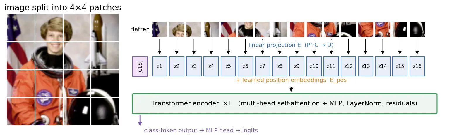
The Vision Transformer [22] removes convolutions almost entirely. An image $\mathbf{x} \in \mathbb{R}^{H \times W \times C}$ is cut into $N = HW/P^2$ non-overlapping $P \times P$ patches. Each patch is flattened and linearly projected to a $D$-dimensional token. A learnable class token is prepended and learnable position embeddings are added:

$$\mathbf{z}_0 = [\,\mathbf{x}_{\text{class}};\; \mathbf{x}_p^1 \mathbf{E};\; \dots;\; \mathbf{x}_p^N \mathbf{E}\,] + \mathbf{E}_{\text{pos}},$$

where $\mathbf{x}_p^i \in \mathbb{R}^{P^2 C}$ is the $i$-th flattened patch, $\mathbf{E} \in \mathbb{R}^{P^2 C \times D}$ the patch embedding and $\mathbf{E}_{\text{pos}} \in \mathbb{R}^{(N+1) \times D}$ the position embeddings. A stack of $L$ standard transformer encoder layers (multi-head self-attention and MLP, each with LayerNorm and a residual connection) processes the sequence, and a small head reads the final class token to produce logits. Self-attention for one head is

$$\operatorname{Attn}(\mathbf{Q}, \mathbf{K}, \mathbf{V}) = \operatorname{softmax}\!\Big(\frac{\mathbf{Q}\mathbf{K}^\top}{\sqrt{d}}\Big)\mathbf{V},$$

with $\mathbf{Q} = \mathbf{Z}\mathbf{W}_Q$, $\mathbf{K} = \mathbf{Z}\mathbf{W}_K$, $\mathbf{V} = \mathbf{Z}\mathbf{W}_V$ linear projections of the token matrix $\mathbf{Z}$, and $d$ the key dimension. The attention matrix is $(N+1) \times (N+1)$: every patch can attend to every other patch from the first layer, so the receptive field is global immediately.

import torch
import torch.nn as nn

B, C, H, W, P, D = 2, 3, 32, 32, 8, 64
img = torch.randn(B, C, H, W)

# 1) patchify: (B, C, H, W) -> (B, N, P*P*C) with N = (H/P)*(W/P)
patches = img.unfold(2, P, P).unfold(3, P, P)                 # (B, C, H/P, W/P, P, P)
patches = patches.permute(0, 2, 3, 1, 4, 5).reshape(B, -1, C * P * P)
N = patches.shape[1]

# 2) linear patch embedding + class token + learned position embedding
embed = nn.Linear(C * P * P, D)          # same as nn.Conv2d(C, D, kernel_size=P, stride=P)
cls = nn.Parameter(torch.zeros(1, 1, D))
pos = nn.Parameter(torch.randn(1, N + 1, D) * 0.02)
z = torch.cat([cls.expand(B, -1, -1), embed(patches)], dim=1) + pos   # (B, N+1, D)

# 3) one head of scaled dot-product self-attention
Wq, Wk, Wv = (nn.Linear(D, D, bias=False) for _ in range(3))
q, k, v = Wq(z), Wk(z), Wv(z)
A = (q @ k.transpose(1, 2) / D ** 0.5).softmax(dim=-1)        # (B, N+1, N+1), rows sum to 1
out = A @ v
print("tokens:", N + 1, " attention:", tuple(A.shape), " class-token output:", tuple(out[:, 0].shape))

Why ViT needs data. A CNN has built-in assumptions, called inductive biases: locality (a pixel mostly relates to its neighbours) and translation equivariance (the same filter everywhere). ViT has almost none; apart from patch extraction and position embeddings, it must learn spatial structure from data. The ViT paper [22] reports that, trained on ImageNet-1k alone, ViTs fell behind comparable ResNets, but pre-trained on much larger datasets (ImageNet-21k or the 300M-image JFT) they matched or beat them. Weak priors cost data at small scale and stop limiting the model at large scale. The same paper also tried hybrid models, feeding the feature map of a ResNet stem into the transformer instead of raw patches; hybrids helped at small compute budgets and the gap closed as models grew.

DeiT: training ViTs on ImageNet alone

DeiT [23] showed that the “ViT needs huge data” conclusion was partly a statement about recipes. With strong augmentation (RandAugment, Mixup, CutMix, random erasing), stochastic depth, repeated augmentation and AdamW, a ViT-B trained only on ImageNet-1k reached 83.1% top-1. DeiT also added a distillation token: a second learnable token, like the class token, whose output is trained to match a teacher network’s predictions (they found a convnet teacher worked best), while the class token is trained on the true label. This is a transformer-specific form of knowledge distillation [51]. At test time the two heads’ outputs are combined.

Swin: windows, shifts and a hierarchy

Global attention costs grow quadratically with the number of tokens, which is a problem for high-resolution inputs and for dense tasks. Swin [24] computes attention only inside non-overlapping $M \times M$ windows, and shifts the window grid by half a window in alternating layers so information crosses window borders. Token count is reduced between stages by merging $2 \times 2$ neighbouring patches, giving a CNN-like pyramid with strides 4, 8, 16, 32. For an $h \times w$ token map with $C$ channels, the paper gives

$$\Omega(\text{MSA}) = 4hwC^2 + 2(hw)^2 C, \qquad \Omega(\text{W-MSA}) = 4hwC^2 + 2M^2 hwC,$$

so windowed attention is linear in the number of tokens $hw$ for a fixed window size $M$. Swin brought back two CNN priors, locality and hierarchy, and became a general-purpose backbone for detection and segmentation as well as classification. The broad landscape of vision transformers is surveyed by Khan et al. [25].

Training recipes

Plain version. The same network can gain or lose several points of accuracy depending on how it is trained. A modern recipe is a bundle of small tricks that each make memorizing harder or optimization smoother.

Data augmentation

• Random resized crop samples a crop covering a random fraction of the image area and a random aspect ratio, then resizes it to the training resolution. It teaches scale and position invariance and is the default for ImageNet training. Horizontal flips are added when they are label-preserving (they are for most photos, not for text or digits).
• Mixup [26] blends two images and their labels: $\tilde{\mathbf{x}} = \lambda \mathbf{x}_i + (1 - \lambda)\mathbf{x}_j$ and $\tilde{\mathbf{y}} = \lambda \mathbf{y}_i + (1 - \lambda)\mathbf{y}_j$, with $\lambda \sim \operatorname{Beta}(\alpha, \alpha)$ and $\mathbf{y}$ one-hot. It encourages linear behaviour between training examples.
• CutMix [27] pastes a random rectangle from image $j$ into image $i$ and mixes the labels in proportion to the pasted area. Unlike Mixup, every pixel stays natural, and the network must recognize objects from partial views.
• RandAugment [28] replaces learned augmentation policies with two numbers: apply $N$ random operations (rotate, shear, posterize, contrast, …) at a shared magnitude $M$. Its paper reports that this tiny search space matches or beats earlier automated policies, and that the right strength depends on model and dataset size.

import numpy as np
import torch
import torch.nn.functional as F

def mixup(x, y, num_classes, alpha=0.2):
    lam = float(np.random.beta(alpha, alpha))
    idx = torch.randperm(x.size(0))
    y1 = F.one_hot(y, num_classes).float()
    return lam * x + (1 - lam) * x[idx], lam * y1 + (1 - lam) * y1[idx]

def cutmix(x, y, num_classes, alpha=1.0):
    lam = float(np.random.beta(alpha, alpha))
    idx = torch.randperm(x.size(0))
    H, W = x.shape[-2:]
    h, w = int(H * np.sqrt(1 - lam)), int(W * np.sqrt(1 - lam))
    cy, cx = np.random.randint(H), np.random.randint(W)
    y0, y1_, x0, x1_ = max(cy - h // 2, 0), min(cy + h // 2, H), max(cx - w // 2, 0), min(cx + w // 2, W)
    x = x.clone()
    x[..., y0:y1_, x0:x1_] = x[idx][..., y0:y1_, x0:x1_]
    lam = 1 - (y1_ - y0) * (x1_ - x0) / (H * W)            # actual area kept
    y1 = F.one_hot(y, num_classes).float()
    return x, lam * y1 + (1 - lam) * y1[idx]

def soft_ce(logits, soft_targets):
    return -(soft_targets * logits.log_softmax(1)).sum(1).mean()

Label smoothing

Cross-entropy with one-hot targets keeps pushing the true logit up forever; the loss only reaches zero at infinite margin. Label smoothing [13] replaces the target with

$$\mathbf{q} = (1 - \varepsilon)\,\mathbf{e}_y + \frac{\varepsilon}{K}\mathbf{1},$$

where $\varepsilon$ (often 0.1) is the smoothing strength, $\mathbf{e}_y$ the one-hot vector and $\mathbf{1}$ the all-ones vector. The optimum is now a finite logit gap, which regularizes the network and usually reduces overconfidence. In PyTorch it is one argument: F.cross_entropy(logits, y, label_smoothing=0.1).

Optimizer, schedule and regularizers

• AdamW [29] decouples weight decay from the adaptive gradient step: instead of adding $\lambda \theta$ to the gradient (which Adam then rescales per parameter), it shrinks the weights directly, $\theta \leftarrow \theta - \eta(\hat{\mathbf{m}}/(\sqrt{\hat{\mathbf{v}}} + \epsilon) + \lambda \theta)$, where $\eta$ is the learning rate, $\hat{\mathbf{m}}, \hat{\mathbf{v}}$ Adam’s moment estimates and $\lambda$ the decay. It is the default for transformers and for modern CNN recipes. Biases and normalization parameters are usually excluded from decay.
• Warmup + cosine schedule. Large learning rates are unstable in the first steps, when normalization statistics and Adam’s moment estimates are still poor, so the learning rate rises linearly for a few epochs. It then follows a half cosine down to near zero, $\eta_t = \tfrac{1}{2}\eta_{\max}(1 + \cos(\pi t / T))$ with $t$ the step after warmup and $T$ the remaining steps, an idea popularized by SGDR [30].
• Stochastic depth [31] randomly skips whole residual branches during training (the block becomes identity), with a skip probability that grows with depth. It shortens the effective depth during training and acts like an ensemble of shallower networks.
• EMA of weights keeps an exponential moving average $\bar{\theta} \leftarrow \mu \bar{\theta} + (1 - \mu)\theta$ (with $\mu$ close to 1, e.g. 0.999) and evaluates $\bar{\theta}$. It smooths out the noise of the last SGD steps.

import math
import torch

def warmup_cosine(step, total, warmup):
    if step < warmup:
        return (step + 1) / warmup                      # linear warmup
    p = (step - warmup) / max(1, total - warmup)
    return 0.5 * (1 + math.cos(math.pi * p))            # cosine decay to 0

model = torch.nn.Linear(10, 3)
decay = [p for n, p in model.named_parameters() if p.ndim > 1]      # weights
no_decay = [p for n, p in model.named_parameters() if p.ndim <= 1]  # biases, norm scales
opt = torch.optim.AdamW([{"params": decay, "weight_decay": 0.05},
                         {"params": no_decay, "weight_decay": 0.0}], lr=1e-3)
total = 1000
sched = torch.optim.lr_scheduler.LambdaLR(opt, lambda s: warmup_cosine(s, total, warmup=50))
ema = torch.optim.swa_utils.AveragedModel(model, multi_avg_fn=torch.optim.swa_utils.get_ema_multi_avg_fn(0.999))
for step in range(total):
    loss = model(torch.randn(16, 10)).pow(2).mean()
    opt.zero_grad(); loss.backward(); opt.step(); sched.step(); ema.update_parameters(model)

A small experiment

To see the pieces working together, we trained a 78k-parameter ResNet (“TinyResNet”: a stem, three basic blocks with 16, 32 and 64 channels, global average pooling) on scikit-learn’s $8 \times 8$ digits, upsampled to $32 \times 32$ so that the strided stages have room to work. To make overfitting visible we used only 100 training images, 500 images for calibration and 1,197 for testing, with AdamW (weight decay 0.05), batch size 32, 40 epochs and two epochs of warmup before a cosine decay. One run used no augmentation. The other used random rotation (±15°), scaling and shifts (a random-resized-crop-like affine; no flips, since a flipped digit is a different symbol) together with label smoothing 0.1. All code is in scripts/figures/dl_02_image_classification.py and runs on a CPU in about a minute.

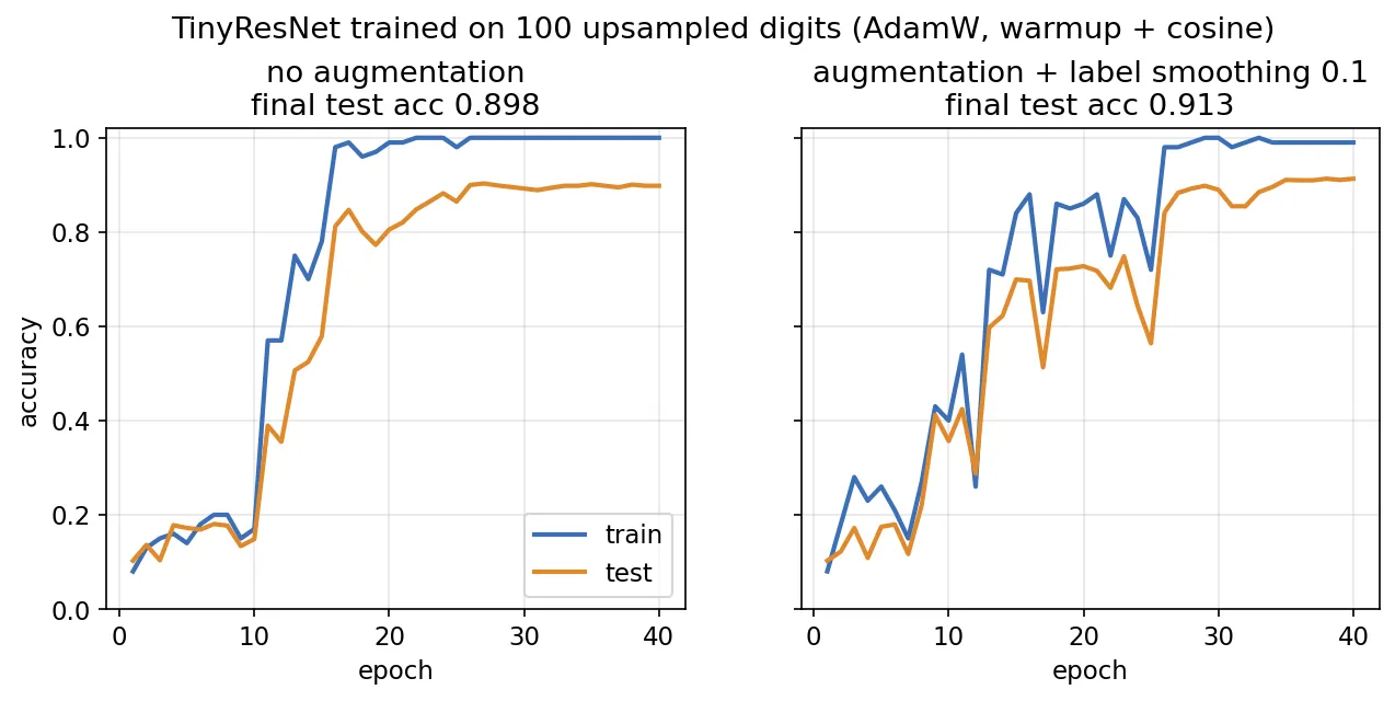
The no-augmentation model reaches 100% training accuracy after about twenty epochs: with 100 images, memorization is easy. The augmented model sees a slightly different version of each digit every epoch, learns more slowly, and generalizes a little better (91.3% against 89.8%). Do not read too much into 1.5 points on one seed; the point is the mechanism.

“ResNet strikes back”

The most striking evidence for recipes comes from Wightman, Touvron and Jégou [32]. They kept the 2015 ResNet-50 architecture fixed and retrained it with a modern recipe: random resized crops and flips, RandAugment, Mixup and CutMix, the LAMB optimizer with a cosine schedule, a binary cross-entropy loss and longer training. The vanilla ResNet-50 reached 80.4% top-1 on ImageNet at $224 \times 224$ without extra data or distillation, against 76.1% for the standard torchvision weights they compare with. Two consequences follow. First, many “new architecture beats ResNet-50” claims compared a new model with a modern recipe against an old model with an old recipe. Second, when you compare architectures, train them with the same, tuned recipe, as ConvNeXt [20] and RegNet [19] did.

Transfer learning and fine-tuning

Plain version. Training a backbone from scratch needs a lot of data. Instead, start from a network already trained on a big dataset and adapt it to your task. You can either keep its features frozen and train only a new last layer, or gently retrain everything.

Let $g_\phi$ be a pre-trained backbone that maps an image to a feature vector $\mathbf{h} = g_\phi(\mathbf{x}) \in \mathbb{R}^{D}$, and $\mathbf{W} \in \mathbb{R}^{K \times D}$ a new linear head.

• Linear probe. Freeze $\phi$ and train only $\mathbf{W}$ (a logistic regression on fixed features). It is cheap, needs few labels, and is the standard way to measure how good a representation is.
• Full fine-tuning. Update $\phi$ and $\mathbf{W}$ together, usually with a learning rate for the backbone 10–100 times smaller than for the head, a short warmup, and sometimes layer-wise learning-rate decay (smaller rates for earlier layers). It adapts the features to the new domain and usually wins when there is enough labelled data.
• In between lie partial fine-tuning (only the last stages), and parameter-efficient methods that add small trainable modules to a frozen backbone.

Kornblith et al. [33] measured how ImageNet accuracy predicts transfer performance. For fine-tuning, better ImageNet models generally transferred better, with a strong correlation. For fixed features, the correlation was weaker and depended on regularization choices: some settings that improved ImageNet accuracy (for example, label smoothing and dropout) produced worse frozen features for other tasks. A good classifier and a good feature extractor are related, but not the same thing.

import torch
import torch.nn as nn

backbone = nn.Sequential(nn.Conv2d(3, 32, 3, 2, 1), nn.ReLU(), nn.Conv2d(32, 64, 3, 2, 1), nn.ReLU(),
                         nn.AdaptiveAvgPool2d(1), nn.Flatten())          # stand-in for a pre-trained model
head = nn.Linear(64, 5)

# linear probe: freeze the backbone, train only the head
for p in backbone.parameters():
    p.requires_grad = False
probe_opt = torch.optim.AdamW(head.parameters(), lr=1e-3)

# full fine-tuning: unfreeze, use a smaller learning rate for the backbone than for the head
for p in backbone.parameters():
    p.requires_grad = True
ft_opt = torch.optim.AdamW([{"params": backbone.parameters(), "lr": 1e-5},
                            {"params": head.parameters(), "lr": 1e-3}], weight_decay=0.05)

Self-supervised and foundation-model classifiers

Plain version. Labels are expensive; images are not. Self-supervised learning invents a task whose answer is in the image itself (are these two crops from the same photo? what was under this mask?), learns features by solving it, and only then uses a few labels.

Contrastive learning: SimCLR and MoCo

Contrastive methods pull together the embeddings of two augmented views of the same image and push apart views of different images. SimCLR [34] takes a batch of $B$ images, makes two random views of each, and minimizes the InfoNCE (NT-Xent) loss for each positive pair $(i, j)$:

$$\ell_{i,j} = -\log \frac{\exp(\operatorname{sim}(\mathbf{z}_i, \mathbf{z}_j)/\tau)}{\sum_{k=1}^{2B} \mathbb{1}_{[k \neq i]} \exp(\operatorname{sim}(\mathbf{z}_i, \mathbf{z}_k)/\tau)},$$

where $\mathbf{z}$ are projected embeddings, $\operatorname{sim}$ is cosine similarity, $\tau$ a temperature and the other $2B - 2$ views in the batch act as negatives. It is a $2B - 1$-way softmax classification: “which of these is my partner?”. SimCLR found that strong augmentation (especially crop plus color distortion), a non-linear projection head and large batches were essential. MoCo [35] avoids the need for huge batches by keeping a queue of negatives encoded by a slowly updated momentum encoder, whose weights are an EMA of the main encoder.

DINO and DINOv2: self-distillation

DINO [36] drops explicit negatives. A student network sees several crops (including small local ones) and is trained to match the output distribution of a teacher that sees global crops. The teacher is an EMA of the student; centering and sharpening of the teacher outputs prevent collapse to a constant. With ViTs, DINO features showed striking properties: the class token’s attention maps segment objects without any segmentation labels, and a simple $k$-NN classifier on frozen features works well. DINOv2 [38] scaled the approach with an automatically curated dataset and a large ViT distilled into smaller ones, producing general-purpose frozen features that work across classification, segmentation and depth without fine-tuning. DINOv3 [39] continued the scaling and introduced “Gram anchoring” to keep dense patch features from degrading during long training.

MAE: masked image modeling

MAE [37] borrows the masked-language-model idea. It masks a large fraction of patches (75% in the paper), feeds only the visible patches to a ViT encoder, and asks a light decoder to reconstruct the missing pixels. Because the encoder skips masked tokens, pre-training is cheap. MAE features are less linearly separable than contrastive ones (linear probes are weaker), but they fine-tune very well. This is a recurring pattern: different pre-training objectives favour different adaptation methods.

CLIP: zero-shot classification with language

CLIP [40] trains an image encoder $g$ and a text encoder $h$ on hundreds of millions of image–caption pairs with a symmetric contrastive loss, so that matching pairs have high cosine similarity. A classifier is then built without any training images: write a prompt per class, such as a photo of a dog., embed it, and predict

$$\hat{y} = \arg\max_{k} \; \frac{g(\mathbf{x})^\top h(t_k)}{\lVert g(\mathbf{x}) \rVert\, \lVert h(t_k) \rVert},$$

where $t_k$ is the prompt for class $k$. The text embeddings act as the weights of a linear classifier, computed from words. The paper reports that zero-shot CLIP matched the accuracy of a ResNet-50 trained on ImageNet’s 1.28M labelled images, and that averaging several prompt templates (“a photo of a …”, “a blurry photo of a …”) helps. Zero-shot accuracy depends strongly on prompt wording, on whether the class names are visually meaningful, and on how well the web data covers the domain.

Robustness and evaluation pitfalls

Plain version. A classifier that scores 90% on its test set may fail badly when the photos come from a different camera, when someone adds invisible noise on purpose, or when the “easy clue” it learned (backgrounds, watermarks) is missing. And even when it is right, its confidence may be wrong.

Distribution shift: ImageNet-C, -R and -A

Hendrycks and colleagues built three widely used shifted test sets for ImageNet classifiers. ImageNet-C [42] applies 15 algorithmic corruptions (noise, blur, weather, digital artefacts) at five severities and summarizes the error relative to a baseline (mean corruption error). ImageNet-R [43] collects renditions (art, cartoons, sculptures, sketches, toys) of 200 ImageNet classes and tests whether a model understands shape and concept rather than photographic texture. ImageNet-A [44] contains natural, unmodified photos that were filtered to fool a ResNet-50; standard models do very poorly on it. These sets reveal different weaknesses, and improving one does not guarantee improving the others. Large-scale pre-training (as in CLIP and DINOv2) tends to improve robustness to such natural shifts much more than architecture changes at fixed data.

Adversarial examples: FGSM

Goodfellow et al. [45] explained adversarial examples by the linearity of networks in high dimensions: a tiny change to every input dimension, aligned with the weights, adds up to a large change in the output. The fast gradient sign method perturbs an input in one step:

$$\mathbf{x}_{\text{adv}} = \operatorname{clip}\big(\mathbf{x} + \varepsilon\, \operatorname{sign}(\nabla_{\mathbf{x}} \mathcal{L}(f_\theta(\mathbf{x}), y))\big),$$

where $\varepsilon$ bounds the change per pixel ($\ell_\infty$ norm), $\mathcal{L}$ is the loss and $\operatorname{clip}$ keeps pixels in the valid range.

import torch.nn.functional as F

def fgsm(model, x, y, eps):
    x = x.clone().requires_grad_(True)
    F.cross_entropy(model(x), y).backward()
    return (x + eps * x.grad.sign()).clamp(-1, 1).detach()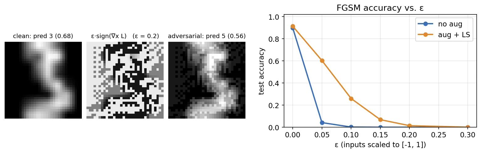

Two cautions about Figure 6. First, the augmented model looks more robust at small $\varepsilon$, but label smoothing is known to flatten the loss surface around training points, which can weaken one-step gradient attacks without giving real robustness; stronger iterative attacks are the proper test. Second, $\varepsilon = 0.05$ on a $[-1, 1]$ scale is visible on an 8×8 digit; on natural images, imperceptible perturbations already fool standard ImageNet models.

Shortcut learning

Geirhos et al. [46] collect many failures under one name: shortcut learning. A network minimizes the training loss with whatever cue is easiest, which is often not the cue we intended: background instead of animal, hospital tag instead of pathology, texture instead of shape. Shortcuts look fine on an i.i.d. test set, because the same shortcut exists there. They fail under distribution shift. The prescription is to test out of distribution on purpose, design tests that break the suspected shortcut, and use interpretability tools such as Grad-CAM (below) to check what the model attends to.

Calibration and temperature scaling

Temperature scaling [47] divides all logits by one scalar $T > 0$ before the softmax, $\mathbf{p} = \operatorname{softmax}(\mathbf{z}/T)$. $T$ is fitted by minimizing the negative log-likelihood on a held-out calibration split (never the test set). $T > 1$ softens overconfident predictions; $T \lt 1$ sharpens underconfident ones. Because dividing by $T$ does not change the argmax, accuracy is unchanged.

import torch
import torch.nn.functional as F

def fit_temperature(logits, y, iters=300):
    """Learn one scalar T > 0 on a held-out calibration split."""
    log_t = torch.zeros(1, requires_grad=True)
    opt = torch.optim.Adam([log_t], lr=0.05)
    for _ in range(iters):
        loss = F.cross_entropy(logits / log_t.exp(), y)
        opt.zero_grad(); loss.backward(); opt.step()
    return log_t.exp().item()

def ece(probs, y, n_bins=10):
    conf, pred = probs.max(1)
    correct = (pred == y).float()
    edges = torch.linspace(0, 1, n_bins + 1)
    total = 0.0
    for lo, hi in zip(edges[:-1], edges[1:]):
        m = (conf > lo) & (conf <= hi)
        if m.any():
            total += m.float().mean() * (correct[m].mean() - conf[m].mean()).abs()
    return float(total)

# toy check: an over-confident "model" = true logits multiplied by 3
torch.manual_seed(0)
true_logits = torch.randn(4000, 10)
y = torch.distributions.Categorical(logits=true_logits).sample()
over = 3 * true_logits
T = fit_temperature(over[:2000], y[:2000])
print(f"T = {T:.2f}  ECE {ece(over[2000:].softmax(1), y[2000:]):.3f} -> "
      f"{ece((over[2000:] / T).softmax(1), y[2000:]):.3f}")
# T = 2.90  ECE 0.345 -> 0.018

In this toy check the logits are three times too large, and the fitted temperature (2.90) recovers that factor. On our real TinyResNet (the model trained without augmentation), the miscalibration went the other way.

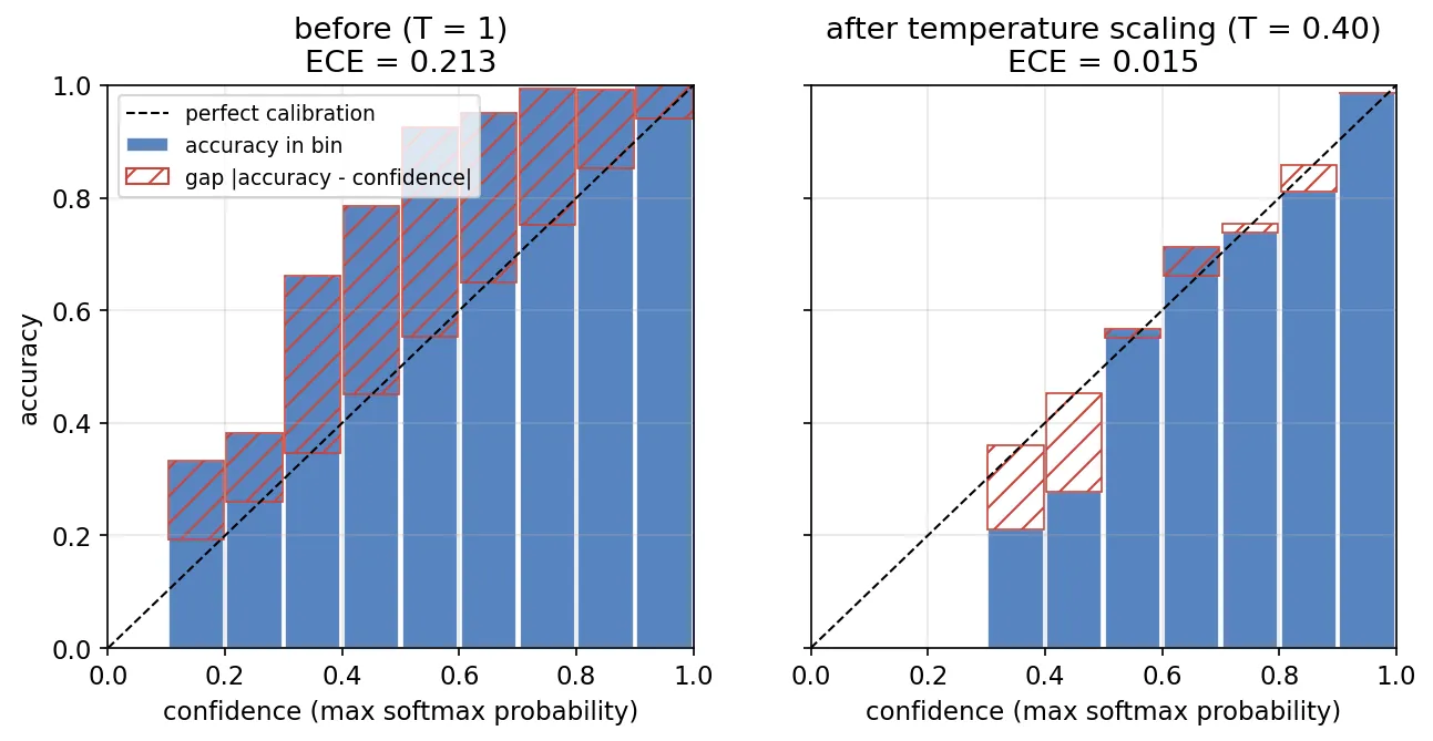
Why underconfident? Our tiny model was trained briefly with strong weight decay, which keeps logits small. Guo et al. [47] observed overconfidence in large, long-trained modern networks, and identified depth, width, batch normalization and reduced weight decay as contributing factors. Miscalibration has no fixed sign; measure it. Also note that calibration is itself fragile under distribution shift: a temperature fitted on in-distribution data does not guarantee calibrated confidence on ImageNet-C-style shifts.

Efficiency

Plain version. A model must fit the device and the time budget. Parameter count, compute, and actual speed are three different measurements, and only the last one is what users feel.

• Parameters determine model size on disk and in memory. A float32 parameter takes 4 bytes.
• FLOPs (or multiply–accumulates, MACs; one MAC is usually counted as two FLOPs) measure arithmetic per image. For a convolution with $K \times K$ kernels, $C_{\text{in}}$ input and $C_{\text{out}}$ output channels on an $H' \times W'$ output map, MACs $= H' W' K^2 C_{\text{in}} C_{\text{out}}$. Compute grows with the square of resolution.
• Latency and throughput are measured on target hardware. Depthwise convolutions have few FLOPs but low arithmetic intensity, so they often run slower on GPUs than their FLOP count suggests; DenseNet’s concatenations cost memory bandwidth. Always benchmark.
• Quantization stores weights and activations as 8-bit integers instead of 32-bit floats. Jacob et al. [50] described integer-only inference with quantization-aware training, which simulates rounding during training so the network learns to tolerate it. Post-training quantization with a small calibration set is the cheap alternative.
• Distillation [51] trains a small student to match a large teacher’s soft predictions, as DeiT did with its distillation token.

Interpretability: CAM and Grad-CAM

Plain version. A heat map over the image shows which regions pushed the score for a class up. It is a sanity check, not a proof of reasoning.

Class activation mapping (CAM) [48] works for networks that end with global average pooling and one linear layer. If $A^k$ is the $k$-th feature map of the last convolutional layer and $w^c_k$ the weight connecting it to class $c$, then the class score is $\sum_k w^c_k \cdot \operatorname{mean}(A^k)$, and the map $\sum_k w^c_k A^k$ shows where that score comes from. Grad-CAM [49] generalizes this to any differentiable architecture by replacing the weights with spatially averaged gradients:

$$\alpha_k^c = \frac{1}{Z}\sum_{i,j} \frac{\partial y^c}{\partial A^k_{ij}}, \qquad L^c_{\text{Grad-CAM}} = \operatorname{ReLU}\Big(\sum_k \alpha_k^c A^k\Big),$$

where $y^c$ is the logit of class $c$, $A^k_{ij}$ the activation of channel $k$ at position $(i, j)$, and $Z$ the number of positions. The ReLU keeps only regions with a positive influence on the class. The coarse map ($8 \times 8$ in our network) is upsampled to the image size.

import torch.nn.functional as F

def grad_cam(model, x, target=None):
    model.eval()
    feats = model.features(x)                          # (1, K, h, w) last conv stage
    feats.retain_grad()
    logits = model.fc(feats.mean(dim=(2, 3)))
    c = logits.argmax(1).item() if target is None else target
    logits[0, c].backward()
    alpha = feats.grad.mean(dim=(2, 3), keepdim=True)  # channel importance weights
    cam = F.relu((alpha * feats).sum(1, keepdim=True))
    cam = F.interpolate(cam, size=x.shape[-2:], mode="bilinear", align_corners=False)
    return (cam / (cam.max() + 1e-8))[0, 0].detach(), c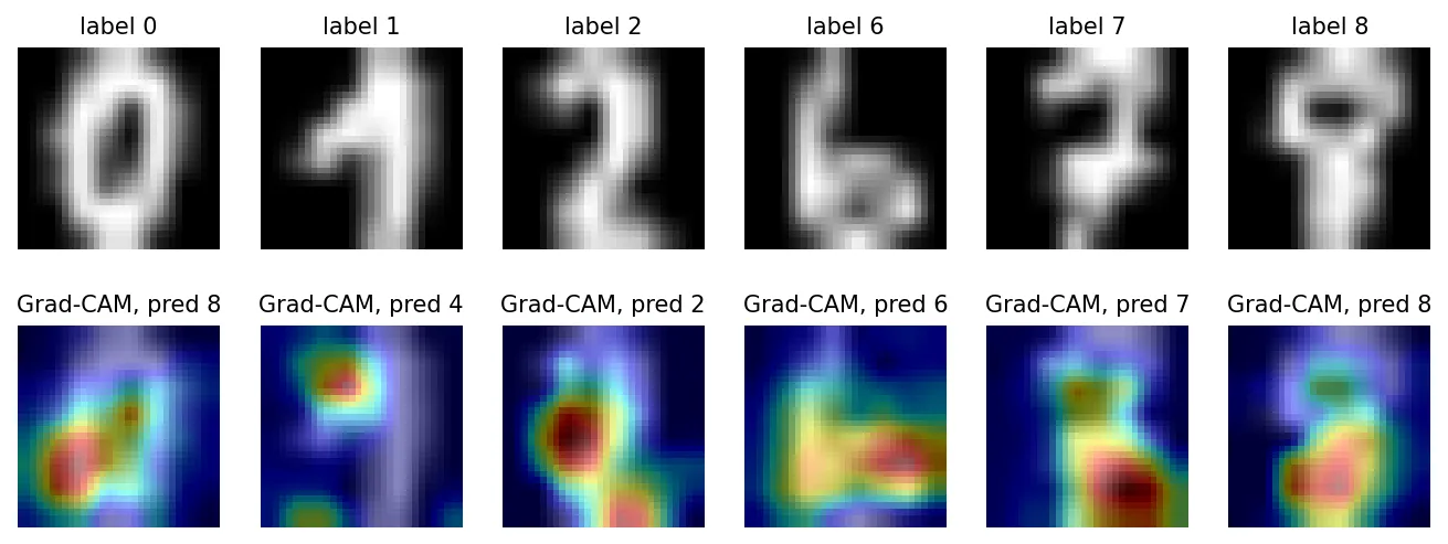

Explanations are most useful exactly when the model is wrong, as in Figure 8: they show which strokes looked like the wrong class. But treat saliency maps with care. They are coarse (limited by the last feature map’s resolution), and they explain one class score for one input, not the model’s general reasoning.

Modern view

Surveys worth reading. Li et al. [1] review CNNs from their history and basic building blocks through classic and advanced models, highlighting the key ideas behind each, and run experiments that compare activation functions, loss functions and optimizers to derive rules of thumb; they close with applications of 1-D, 2-D and multi-dimensional convolution and a list of open issues. Khan et al. [25] survey vision transformers across tasks. For classification they group them into uniform-scale models (ViT, DeiT), multi-scale hierarchical models (such as Swin), hybrids with convolutions, and self-supervised transformers (such as DINO), and they stress the reliance on large-scale pre-training and the cost of quadratic attention. Gui et al. [41] survey self-supervised learning and divide it into context-based methods (pretext tasks such as rotation prediction or jigsaw puzzles), contrastive methods (with negative pairs, self-distillation as in DINO, or feature decorrelation), generative methods (masked image modeling as in MAE), and hybrids of contrastive and generative objectives, before covering combinations with semi-supervised and multi-modal learning. On the reliability of benchmarks, the ImageNetV2 study [7], the re-labelling study of Beyer et al. [8] and the label-error analysis of Northcutt et al. [9] together argue for multiple test sets, multi-label evaluation and reporting variance.

The 2023–2026 picture. Five trends define current practice.

1. Pre-train once, adapt cheaply. Most new classifiers are not trained from scratch. They start from a large backbone trained with self-supervision (DINOv2 [38], DINOv3 [39]), image–text contrast (CLIP [40] and open reproductions), or masked modeling (MAE [37]), and adapt it with a linear probe, a $k$-NN rule, or a short fine-tune.
2. Zero-shot and open-vocabulary classification. Image–text models turn the label set into text. The class list can change at test time without retraining, which blurs the line between classification and retrieval.
3. Scaling laws for vision. Zhai et al. [52] scaled ViTs to billions of parameters and characterized how error falls with compute, data and model size, including the observation that larger models are more sample-efficient in few-shot transfer. Cherti et al. [53] fitted reproducible power laws for open CLIP training on public data, and found that the scaling behaviour depends on the training data distribution and the downstream task.
4. Architectures converged. ConvNeXt [20] and Swin [24] show that convolutions and attention, given the same recipe and scale, land in a similar place. The choice is now driven by hardware, resolution and downstream tasks (dense prediction favours hierarchical designs) more than by top-1 accuracy.
5. Evaluation moved beyond ImageNet-1k top-1. Robustness suites (ImageNet-C/R/A [42]–[44] and ImageNetV2 [7]), calibration, and transfer to many downstream datasets are now standard parts of a backbone paper.

Open problems. Robustness to natural distribution shift still lags clean accuracy, and gains from robust training methods are often specific to the shift they target. Shortcut learning [46] is hard to detect without counterfactual tests. Calibration under shift is unsolved. Long-tailed and fine-grained recognition remain hard because the rare classes have the fewest examples. Benchmark saturation and label noise make small accuracy differences on ImageNet-1k uninformative. And the dominant foundation models are trained on web-scale data whose composition, licensing and biases are hard to audit, which matters directly for what a “zero-shot” classifier will and will not recognize.

Key takeaways

• A classifier outputs logits; softmax + cross-entropy trains single-label tasks, independent sigmoids + binary cross-entropy train multi-label tasks. Report top-1 accuracy and, where it matters, calibration (ECE) and per-class results.
• Each landmark CNN fixed one bottleneck: ReLU/GPUs (AlexNet), small stacked kernels (VGG), $1 \times 1$ reductions and multi-branch modules (Inception), identity shortcuts for optimization (ResNet), depthwise separable convolutions for cost (MobileNet), balanced scaling (EfficientNet).
• ViTs trade convolutional inductive biases for flexibility; they need more data or a stronger recipe (DeiT), and windows plus hierarchy (Swin) make them practical backbones. ConvNeXt shows that the recipe explains much of the gap.
• Training recipes matter as much as architecture: augmentation (random resized crop, Mixup, CutMix, RandAugment), label smoothing, AdamW, warmup + cosine, stochastic depth and EMA lifted an unchanged ResNet-50 to 80.4% top-1.
• Pre-trained backbones are the default starting point. Linear probes measure representations; fine-tuning adapts them. CLIP turns class names into classifier weights for zero-shot recognition.
• Benchmark accuracy is fragile: test on shifted data, beware shortcuts and adversarial inputs, fit a temperature on held-out data, and inspect Grad-CAM maps, especially on errors.

Exercises

1. Receptive fields and parameters. Show that three stacked $3 \times 3$ convolutions (stride 1) have a $7 \times 7$ receptive field. With $C$ input and output channels and no biases, compare their parameter count with a single $7 \times 7$ convolution.

Hint

Each $3 \times 3$ layer adds 2 pixels to the receptive field: $3 \to 5 \to 7$. Parameters: $3 \cdot 9C^2 = 27C^2$ versus $49C^2$, about 45% fewer, plus two extra nonlinearities.

2. Bottleneck arithmetic. A ResNet bottleneck has $4d$ input channels and reduces to $d$. Count the weights (no biases) of the $1 \times 1$–$3 \times 3$–$1 \times 1$ branch as a function of $d$, and compare with a basic block of two $3 \times 3$ convolutions at width $4d$. What is the ratio?

Hint

Bottleneck: $4d \cdot d + 9d^2 + d \cdot 4d = 17d^2$. Basic block at width $4d$: $2 \cdot 9 \cdot 16d^2 = 288d^2$. The ratio is $17/288 \approx 0.059$, about 17 times fewer weights.

3. Label smoothing optimum. For one example with $K$ classes and smoothing $\varepsilon$, assume all wrong-class logits are equal. Show that the cross-entropy with smoothed targets is minimized when the logit gap between the true class and each wrong class is $\log\big((1 - \varepsilon + \varepsilon/K)\,/\,(\varepsilon/K)\big)$. Evaluate it for $K = 1000$, $\varepsilon = 0.1$.

Hint

The minimum of cross-entropy over $\mathbf{p}$ is at $\mathbf{p} = \mathbf{q}$. So $p_y = 1 - \varepsilon + \varepsilon/K$ and every other $p_k = \varepsilon/K$, and the logit gap is the log of their ratio: $\log(0.9001 / 0.0001) \approx 9.1$. Without smoothing the optimal gap is infinite.

4. ViT token count. A ViT with $16 \times 16$ patches receives a $224 \times 224$ image. How many tokens enter the encoder? If the image is fine-tuned at $384 \times 384$, how many tokens are there, by what factor does the attention-matrix size grow, and what must be done with the position embeddings?

Hint

$(224/16)^2 = 196$ patches plus one class token: 197. At 384: $24^2 + 1 = 577$. The attention matrix grows by $(577/197)^2 \approx 8.6$. The learned position embeddings form a $14 \times 14$ grid; they are interpolated (2-D) to $24 \times 24$, which is what the ViT paper does when fine-tuning at higher resolution.

5. Temperature does not change accuracy. Prove that for any $T > 0$, $\arg\max_k \operatorname{softmax}(\mathbf{z}/T)_k = \arg\max_k z_k$. Then, using scripts/figures/dl_02_image_classification.py, fit the temperature on the test set instead of the calibration split and compare the reported ECE. Why is that number optimistic?

Hint

Division by a positive constant and the exponential are both strictly increasing, and the softmax denominator is shared. Fitting $T$ on the test set uses test labels to tune a parameter, so the reported ECE is no longer an honest estimate of performance on new data.

6. Build a shortcut. Modify the digit experiment so that in the training set every “3” has a bright pixel in the top-left corner, but the test set does not. Train the TinyResNet, report test accuracy on the 3s, and look at Grad-CAM maps for a few training 3s. What do you expect, and how would you detect this problem if you did not know the shortcut was there?

Hint

The network can classify training 3s from the corner pixel alone, so test accuracy on 3s drops while training accuracy stays perfect, and Grad-CAM tends to highlight the corner. Without knowing the shortcut, look for heat maps that fall on background, evaluate on independently collected data, and run counterfactual tests (erase or move suspicious regions and see whether predictions change).

References

1. Z. Li, F. Liu, W. Yang, S. Peng, and J. Zhou, “A Survey of Convolutional Neural Networks: Analysis, Applications, and Prospects,” IEEE Transactions on Neural Networks and Learning Systems, vol. 33, no. 12, pp. 6999–7019, 2022. doi:10.1109/TNNLS.2021.3084827
2. O. Russakovsky, J. Deng, H. Su, J. Krause, S. Satheesh, S. Ma, et al., “ImageNet Large Scale Visual Recognition Challenge,” International Journal of Computer Vision, vol. 115, pp. 211–252, 2015. doi:10.1007/s11263-015-0816-y
3. Y. LeCun, L. Bottou, Y. Bengio, and P. Haffner, “Gradient-Based Learning Applied to Document Recognition,” Proceedings of the IEEE, vol. 86, no. 11, pp. 2278–2324, 1998. doi:10.1109/5.726791
4. A. Krizhevsky, “Learning Multiple Layers of Features from Tiny Images,” technical report, University of Toronto, 2009. dataset page
5. T. Ridnik, E. Ben-Baruch, A. Noy, and L. Zelnik-Manor, “ImageNet-21K Pretraining for the Masses,” NeurIPS, 2021. arXiv
6. G. Van Horn, O. Mac Aodha, Y. Song, Y. Cui, C. Sun, A. Shepard, et al., “The iNaturalist Species Classification and Detection Dataset,” CVPR, 2018. arXiv
7. B. Recht, R. Roelofs, L. Schmidt, and V. Shankar, “Do ImageNet Classifiers Generalize to ImageNet?,” ICML, PMLR vol. 97, 2019. paper
8. L. Beyer, O. J. Hénaff, A. Kolesnikov, X. Zhai, and A. van den Oord, “Are We Done with ImageNet?,” arXiv:2006.07159, 2020. arXiv
9. C. G. Northcutt, A. Athalye, and J. Mueller, “Pervasive Label Errors in Test Sets Destabilize Machine Learning Benchmarks,” NeurIPS, 2021. arXiv
10. A. Krizhevsky, I. Sutskever, and G. E. Hinton, “ImageNet Classification with Deep Convolutional Neural Networks,” Advances in Neural Information Processing Systems 25 (NIPS), 2012. paper
11. K. Simonyan and A. Zisserman, “Very Deep Convolutional Networks for Large-Scale Image Recognition,” ICLR, 2015. arXiv
12. C. Szegedy, W. Liu, Y. Jia, P. Sermanet, S. Reed, D. Anguelov, D. Erhan, V. Vanhoucke, and A. Rabinovich, “Going Deeper with Convolutions,” CVPR, 2015. doi:10.1109/CVPR.2015.7298594
13. C. Szegedy, V. Vanhoucke, S. Ioffe, J. Shlens, and Z. Wojna, “Rethinking the Inception Architecture for Computer Vision,” CVPR, 2016. doi:10.1109/CVPR.2016.308
14. K. He, X. Zhang, S. Ren, and J. Sun, “Deep Residual Learning for Image Recognition,” CVPR, 2016. doi:10.1109/CVPR.2016.90
15. K. He, X. Zhang, S. Ren, and J. Sun, “Identity Mappings in Deep Residual Networks,” ECCV, 2016. arXiv
16. G. Huang, Z. Liu, L. van der Maaten, and K. Q. Weinberger, “Densely Connected Convolutional Networks,” CVPR, 2017. arXiv
17. A. G. Howard, M. Zhu, B. Chen, D. Kalenichenko, W. Wang, T. Weyand, M. Andreetto, and H. Adam, “MobileNets: Efficient Convolutional Neural Networks for Mobile Vision Applications,” arXiv:1704.04861, 2017. arXiv
18. M. Tan and Q. V. Le, “EfficientNet: Rethinking Model Scaling for Convolutional Neural Networks,” ICML, 2019. arXiv
19. I. Radosavovic, R. P. Kosaraju, R. Girshick, K. He, and P. Dollár, “Designing Network Design Spaces,” CVPR, 2020. arXiv
20. Z. Liu, H. Mao, C.-Y. Wu, C. Feichtenhofer, T. Darrell, and S. Xie, “A ConvNet for the 2020s,” CVPR, 2022. arXiv
21. J. Hu, L. Shen, S. Albanie, G. Sun, and E. Wu, “Squeeze-and-Excitation Networks,” arXiv:1709.01507, 2017 (journal version in IEEE TPAMI). arXiv
22. A. Dosovitskiy, L. Beyer, A. Kolesnikov, D. Weissenborn, X. Zhai, T. Unterthiner, et al., “An Image is Worth 16x16 Words: Transformers for Image Recognition at Scale,” ICLR, 2021. arXiv
23. H. Touvron, M. Cord, M. Douze, F. Massa, A. Sablayrolles, and H. Jégou, “Training Data-Efficient Image Transformers & Distillation through Attention,” ICML, PMLR vol. 139, 2021. paper
24. Z. Liu, Y. Lin, Y. Cao, H. Hu, Y. Wei, Z. Zhang, S. Lin, and B. Guo, “Swin Transformer: Hierarchical Vision Transformer using Shifted Windows,” ICCV, 2021. doi:10.1109/ICCV48922.2021.00986
25. S. Khan, M. Naseer, M. Hayat, S. W. Zamir, F. S. Khan, and M. Shah, “Transformers in Vision: A Survey,” ACM Computing Surveys, 2022. arXiv
26. H. Zhang, M. Cisse, Y. N. Dauphin, and D. Lopez-Paz, “mixup: Beyond Empirical Risk Minimization,” ICLR, 2018. arXiv
27. S. Yun, D. Han, S. J. Oh, S. Chun, J. Choe, and Y. Yoo, “CutMix: Regularization Strategy to Train Strong Classifiers with Localizable Features,” ICCV, 2019. arXiv
28. E. D. Cubuk, B. Zoph, J. Shlens, and Q. V. Le, “RandAugment: Practical Automated Data Augmentation with a Reduced Search Space,” CVPR Workshops, 2020. doi:10.1109/CVPRW50498.2020.00359
29. I. Loshchilov and F. Hutter, “Decoupled Weight Decay Regularization,” ICLR, 2019. arXiv
30. I. Loshchilov and F. Hutter, “SGDR: Stochastic Gradient Descent with Warm Restarts,” ICLR, 2017. arXiv
31. G. Huang, Y. Sun, Z. Liu, D. Sedra, and K. Q. Weinberger, “Deep Networks with Stochastic Depth,” ECCV, 2016. doi:10.1007/978-3-319-46493-0_39
32. R. Wightman, H. Touvron, and H. Jégou, “ResNet Strikes Back: An Improved Training Procedure in timm,” arXiv:2110.00476, 2021. arXiv
33. S. Kornblith, J. Shlens, and Q. V. Le, “Do Better ImageNet Models Transfer Better?,” CVPR, 2019. arXiv
34. T. Chen, S. Kornblith, M. Norouzi, and G. Hinton, “A Simple Framework for Contrastive Learning of Visual Representations,” ICML, 2020. arXiv
35. K. He, H. Fan, Y. Wu, S. Xie, and R. Girshick, “Momentum Contrast for Unsupervised Visual Representation Learning,” CVPR, 2020. arXiv
36. M. Caron, H. Touvron, I. Misra, H. Jégou, J. Mairal, P. Bojanowski, and A. Joulin, “Emerging Properties in Self-Supervised Vision Transformers,” ICCV, 2021. doi:10.1109/ICCV48922.2021.00951
37. K. He, X. Chen, S. Xie, Y. Li, P. Dollár, and R. Girshick, “Masked Autoencoders Are Scalable Vision Learners,” CVPR, 2022. doi:10.1109/CVPR52688.2022.01553
38. M. Oquab, T. Darcet, T. Moutakanni, H. Vo, M. Szafraniec, V. Khalidov, et al., “DINOv2: Learning Robust Visual Features without Supervision,” Transactions on Machine Learning Research, 2024. arXiv
39. O. Siméoni, H. V. Vo, M. Seitzer, F. Baldassarre, M. Oquab, C. Jose, et al., “DINOv3,” arXiv:2508.10104, 2025. arXiv
40. A. Radford, J. W. Kim, C. Hallacy, A. Ramesh, G. Goh, S. Agarwal, et al., “Learning Transferable Visual Models From Natural Language Supervision,” ICML, PMLR vol. 139, 2021. paper
41. J. Gui, T. Chen, J. Zhang, Q. Cao, Z. Sun, H. Luo, and D. Tao, “A Survey on Self-Supervised Learning: Algorithms, Applications, and Future Trends,” IEEE Transactions on Pattern Analysis and Machine Intelligence (arXiv:2301.05712, 2023). arXiv
42. D. Hendrycks and T. Dietterich, “Benchmarking Neural Network Robustness to Common Corruptions and Perturbations,” ICLR, 2019. arXiv
43. D. Hendrycks, S. Basart, N. Mu, S. Kadavath, F. Wang, E. Dorundo, et al., “The Many Faces of Robustness: A Critical Analysis of Out-of-Distribution Generalization,” ICCV, 2021. arXiv
44. D. Hendrycks, K. Zhao, S. Basart, J. Steinhardt, and D. Song, “Natural Adversarial Examples,” CVPR, 2021. arXiv
45. I. J. Goodfellow, J. Shlens, and C. Szegedy, “Explaining and Harnessing Adversarial Examples,” in Proc. International Conference on Learning Representations (ICLR), 2015. arXiv
46. R. Geirhos, J.-H. Jacobsen, C. Michaelis, R. Zemel, W. Brendel, M. Bethge, and F. A. Wichmann, “Shortcut Learning in Deep Neural Networks,” Nature Machine Intelligence, 2020. arXiv
47. C. Guo, G. Pleiss, Y. Sun, and K. Q. Weinberger, “On Calibration of Modern Neural Networks,” ICML, 2017. arXiv
48. B. Zhou, A. Khosla, A. Lapedriza, A. Oliva, and A. Torralba, “Learning Deep Features for Discriminative Localization,” CVPR, 2016. doi:10.1109/CVPR.2016.319
49. R. R. Selvaraju, M. Cogswell, A. Das, R. Vedantam, D. Parikh, and D. Batra, “Grad-CAM: Visual Explanations from Deep Networks via Gradient-Based Localization,” ICCV, 2017. doi:10.1109/ICCV.2017.74
50. B. Jacob, S. Kligys, B. Chen, M. Zhu, M. Tang, A. Howard, et al., “Quantization and Training of Neural Networks for Efficient Integer-Arithmetic-Only Inference,” CVPR, 2018. doi:10.1109/CVPR.2018.00286
51. G. Hinton, O. Vinyals, and J. Dean, “Distilling the Knowledge in a Neural Network,” arXiv:1503.02531, 2015. arXiv
52. X. Zhai, A. Kolesnikov, N. Houlsby, and L. Beyer, “Scaling Vision Transformers,” CVPR, 2022. arXiv
53. M. Cherti, R. Beaumont, R. Wightman, M. Wortsman, G. Ilharco, C. Gordon, et al., “Reproducible Scaling Laws for Contrastive Language-Image Learning,” CVPR, 2023. arXiv