DL 04 · Deep Image Restoration: Low-Level Vision

What you’ll learn

• What “low-level vision” means, and why super-resolution, denoising, deblurring, dehazing, deraining, desnowing and low-light enhancement are really one problem: invert a degradation $y = \mathcal D(x) + n$.
• How deep restoration is set up in practice: paired data, synthetic degradation pipelines, and the gap to real-world (blind) degradations. You will build a pipeline and train a tiny residual denoiser in PyTorch.
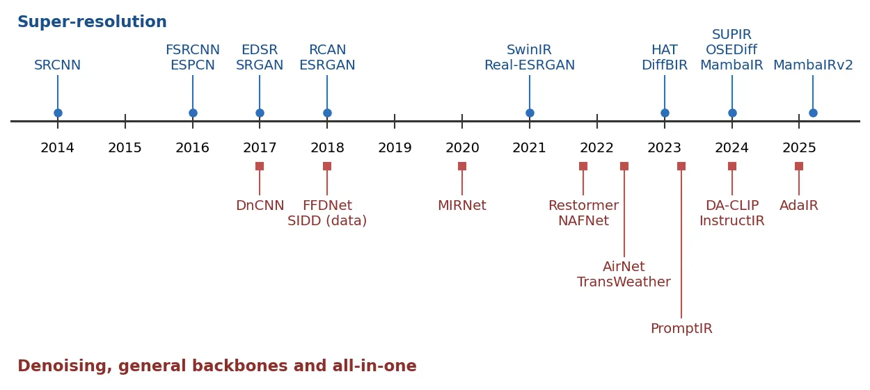
• The milestones and current families for each task, from SRCNN, DnCNN, DehazeNet and the GoPro deblurring benchmark to SwinIR, Restormer, NAFNet, MambaIR and diffusion-based SR (SUPIR, OSEDiff).
• How all-in-one models (AirNet, TransWeather, PromptIR, AdaIR, DA-CLIP, InstructIR) handle unknown or mixed degradations with one network.
• Which losses and metrics to use, why PSNR and “looks real” disagree (the perception–distortion trade-off), and how NTIRE challenges track the field.

The big picture

Low-level vision is about the pixels themselves. Before a system can recognize a face, read a sign or detect a car, the image has to be clear enough to look at. Restoration models are the part of the pipeline that takes a damaged photo (too small, noisy, blurred, foggy, rainy, dark) and returns a better estimate of the clean scene.

Why it matters: every phone camera runs denoising, demosaicking and super-resolution before you ever see a picture. Satellite, microscope, medical and surveillance images are restored before they are measured. Video streaming services upscale low-bitrate frames. Self-driving cars need their detectors to work in rain and fog. And from a research point of view, restoration is where many architectural ideas were tested first: residual learning, channel attention, efficient transformers and diffusion priors all have well-known restoration variants.

We assume you know CNNs and backpropagation (DL 01) and the classical restoration chapter (DIP 5), which covers noise models, Wiener filtering and the degradation model in detail. We link to it rather than repeat it.

What is low-level vision?

Plain version. High-level vision asks “what is in the picture?” (classification, detection). Low-level vision asks “what does the picture actually look like, pixel by pixel?” One is about understanding, the other about perceiving.

The analogy in the author’s post [1] comes from how people interact with the world: we first sense (light hits the retina and we see edges, colors and contrast) and then interpret (that is a cup). Both are necessary. If the sensing is poor (the cup is blurry), the interpretation suffers. Low-level vision tasks exist to make the sensing good again: when we say an object looks “blurry”, our perception of it is not sharp, and a deblurring task is created to make it “clear”.

Precise version. A low-level vision task maps an image to an image of (usually) the same content:

$$f_\theta : \mathbb R^{H \times W \times C} \to \mathbb R^{H' \times W' \times C'},$$

where the output is a pixel-wise estimate rather than a label. $H, W, C$ are the input height, width and channels, and $H', W', C'$ those of the output ($H' = sH$ for super-resolution by a factor $s$, otherwise usually equal). This has three consequences that shape the whole field:

1. Dense, high-resolution outputs. Every pixel matters, so architectures cannot downsample aggressively and must keep fine detail, which makes them expensive at high resolution.
2. Supervision is cheap to synthesize. Take a clean image, damage it with a known process, and you have an input–target pair. This is a huge advantage over labeled data for recognition, and also the source of the field’s main weakness (synthetic damage is not real damage).
3. “Correct” is ambiguous. Many clean images are consistent with one damaged image. Which one is “best” depends on whether you value fidelity to the truth or natural appearance, as we will see in the evaluation section.

The family of tasks is broad: deblurring, super-resolution, denoising, inpainting, color calibration, infrared–visible fusion and more. Papers with Code used to be the standard place to browse these task lists and leaderboards, but it has shut down and its address now redirects to Hugging Face’s trending-papers page, so its per-task leaderboards are no longer available. A reliable way to follow progress today is the yearly NTIRE challenge reports (New Trends in Image Restoration and Enhancement, a CVPR workshop), which we discuss near the end [2], [3].

One problem, many faces: the degradation model

Plain version. Every task in this tutorial can be written as “the camera saw a clean scene $x$, something damaged it, and we got $y$.” Only the damage changes. If you can write the damage down, you can name the task.

The unified view

$$y = \mathcal D(x) + n,$$

where $x$ is the unknown clean image, $\mathcal D$ is a (possibly nonlinear, possibly unknown) degradation operator, $n$ is noise, and $y$ is what we observe. Restoration means estimating $x$ from $y$. Here are the specific forms used in the post [1] and in the rest of this tutorial. Figure 1 shows each one applied to the same photo.

Blur (the textbook model). As in DIP 5,

$$g(u, v) = (h * f)(u, v) + n(u, v),$$

where $f$ is the sharp image, $h$ the point spread function (blur kernel), $*$ 2-D convolution, $n$ additive noise and $g$ the observed image, all indexed by pixel coordinates $(u, v)$. Denoising is the special case $h = \delta$ (a unit impulse, so no blur).

Super-resolution. The low-resolution image is a blurred, subsampled and noisy version of the high-resolution one:

$$y = (x * k)\downarrow_s + n,$$

where $k$ is a blur (anti-aliasing) kernel, $\downarrow_s$ keeps every $s$-th pixel in each direction, and $s$ is the scale factor (2, 3, 4, …). The classic “bicubic” benchmark setting replaces all of this with MATLAB-style bicubic downsampling and no noise.

Compression. $y = \mathrm{JPEG}_q(x)$, where $q$ is the quality factor. JPEG quantizes $8 \times 8$ DCT coefficients (see DIP 8), producing blocking and ringing. It is not additive and not linear, so it is usually just added to the pipeline as a black box.

Haze (the atmospheric scattering model).

$$I(p) = J(p)\, t(p) + A\,\bigl(1 - t(p)\bigr), \qquad t(p) = e^{-\beta d(p)},$$

where $p$ is a pixel, $I$ the hazy image, $J$ the haze-free scene radiance, $A$ the global atmospheric light (the color of the haze), $t \in (0, 1]$ the transmission, $\beta$ the scattering coefficient and $d$ the scene depth. The first term is the attenuated scene; the second is “airlight” scattered toward the camera. Far objects (large $d$) get small $t$ and fade into $A$.

Rain. For rain streaks the common model is additive,

$$I = B + R,$$

where $B$ is the rain-free background and $R$ the rain layer. Raindrops stuck on a lens or windshield behave differently: they block and refract the background, so a popular model is $I = (1 - M) \odot B + R$, where $M$ is a binary raindrop mask, $\odot$ the element-wise product and $R$ the light passing through the drops [39].

Low light (Retinex). Retinex theory [5] separates an image into reflectance and illumination:

$$S = R \cdot L,$$

where $S$ is the observed image, $R$ the reflectance (the intrinsic color and texture of surfaces, what we want), $L$ the illumination and $\cdot$ the element-wise product. A dark photo has small $L$; enhancement estimates $L$ and brightens it, while noise that was hidden in the dark gets amplified.

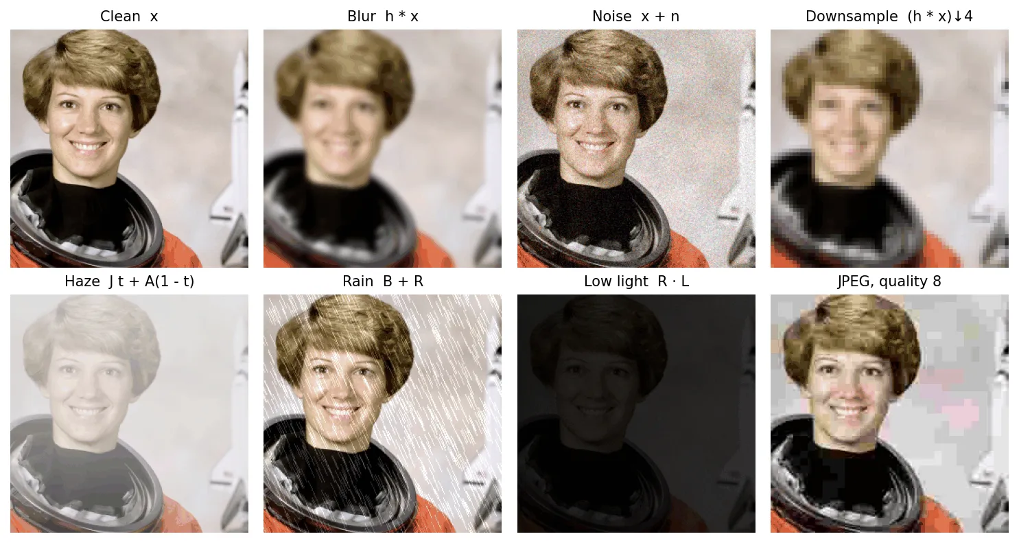
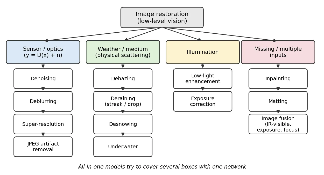
Although none of these models is exact, they all have the same shape: a clean image goes in, an operator plus noise comes out. That is the post’s central point [1]: seen through the degradation model, these are all the same kind of problem, and the same tools (and often the same networks) apply to all of them. Figure 2 organizes them by where the damage comes from.

Why the problem is hard: ill-posedness

For almost every $\mathcal D$ above, many different $x$ produce the same $y$. Downsampling by 4 throws away 15 of every 16 pixels; blur suppresses high frequencies to near zero; haze with $t \approx 0$ erases distant objects. The inverse problem is ill-posed, and we need a prior on what clean images look like. In the Bayesian (MAP) form,

$$\hat x = \arg\min_x \; \tfrac{1}{2}\bigl\| y - \mathcal D(x) \bigr\|_2^2 + \lambda\, \Phi(x),$$

where the first term (data fidelity) says ”$\hat x$ must explain the observation”, $\Phi$ is a regularizer encoding the prior (small $\Phi$ for natural-looking images), and $\lambda > 0$ balances the two. The whole history of the field is a history of better priors $\Phi$.

Before deep learning: the era of hand-crafted priors

Before deep learning, each task had its own carefully reasoned prior, and success depended on having enough physical or statistical knowledge of the problem. Denoising used local smoothness, non-local self-similarity and sparsity; deblurring used Wiener and constrained least-squares filters plus heavy-tailed gradient priors; dehazing used the dark channel prior [25]; super-resolution used interpolation and example-based dictionaries; low-light enhancement used histogram equalization and Retinex decompositions. DIP 5 covers the core of this toolbox (noise models, mean/median/adaptive filters, inverse, Wiener and CLS filtering) and ends with a short history of the move to learned denoisers. The author’s view in [1] is that once deep learning surpassed what these models could do, the decisive factor stopped being a strong theoretical prior for each task and became a strong learning mechanism and feature extractor. The degradation model did not disappear: it moved from the solver into the data generator.

The deep learning formulation

Plain version. Make lots of (damaged, clean) pairs, and train a network to map damaged to clean. Most of the hard work is in making the damage realistic.

Supervised training on pairs

Given a dataset of clean images $\{x_i\}$ and a degradation sampler, we build pairs $(y_i, x_i)$ with $y_i = \mathcal D_i(x_i) + n_i$, and fit

$$\theta^\star = \arg\min_\theta \; \frac{1}{N} \sum_{i=1}^{N} \ell\bigl(f_\theta(y_i),\, x_i\bigr),$$

where $f_\theta$ is the restoration network with parameters $\theta$, $N$ the number of training pairs and $\ell$ a loss (L1, L2, perceptual, adversarial, …; see the losses section). Training is done on random crops (“patches”, e.g. $64 \times 64$ to $256 \times 256$) with flips and rotations, because convolutional and windowed-attention networks are translation-equivariant and full-resolution images do not fit in GPU memory.

A useful fact explains a lot of what follows: with the L2 loss, the optimal network outputs the posterior mean $f^\star(y) = \mathbb E[x \mid y]$. When many sharp images are consistent with $y$, their average is blurry. This is why MSE-trained super-resolution looks smooth, and why GANs and diffusion models were brought in.

Synthetic degradation pipelines

Pairs come from three sources. (1) Synthetic: degrade clean images with a known model (bicubic downsampling, Gaussian noise, Gaussian blur, JPEG). Cheap and unlimited, but limited by how realistic the model is. (2) Captured: photograph the same scene twice, e.g. a short and a long exposure, or a burst averaged into a clean reference (as in the SIDD real-noise dataset [22]), or averaging high-speed video frames to create real motion blur (GoPro [44]). Realistic but expensive and specific to one camera. (3) Unpaired / self-supervised: learn from degraded images alone, using GANs, cycle consistency or noise statistics. Most strong models today train on synthetic pairs from a rich degradation pipeline and evaluate on both synthetic and captured data.

A typical “classic” pipeline is blur → downsample → noise → JPEG, mirroring the order in which a camera and an image-sharing site would damage a photo:

import numpy as np, cv2, torch, torch.nn.functional as F
from skimage import data, img_as_float32

def gaussian_kernel(sigma, size=21):
    ax = torch.arange(size) - size // 2
    g = torch.exp(-ax**2 / (2 * sigma**2))
    k = torch.outer(g, g)
    return k / k.sum()

def degrade(x, scale=4, sigma_blur=1.6, sigma_noise=0.03, jpeg_q=40, rng=None):
    """x: float tensor (C,H,W) in [0,1]. Returns the low-quality image y = D(x) + n."""
    rng = rng or np.random.default_rng(0)
    C = x.shape[0]
    k = gaussian_kernel(sigma_blur).to(x)[None, None].repeat(C, 1, 1, 1)
    y = F.conv2d(F.pad(x[None], (10,) * 4, mode="reflect"), k, groups=C)   # 1) blur  h * x
    y = y[..., ::scale, ::scale]                                           # 2) downsample  (.)↓s
    y = y + sigma_noise * torch.from_numpy(rng.standard_normal(y.shape).astype(np.float32))  # 3) noise n
    y = y.clamp(0, 1)[0]
    img = (y.permute(1, 2, 0).numpy() * 255).round().astype(np.uint8)      # 4) JPEG round trip
    ok, buf = cv2.imencode(".jpg", img[..., ::-1], [cv2.IMWRITE_JPEG_QUALITY, jpeg_q])
    img = cv2.imdecode(buf, cv2.IMREAD_COLOR)[..., ::-1]
    return torch.from_numpy(img.copy()).permute(2, 0, 1).float() / 255

x = torch.from_numpy(img_as_float32(data.astronaut())).permute(2, 0, 1)    # (3, 512, 512)
y = degrade(x)
print(x.shape, "->", y.shape)        # torch.Size([3, 512, 512]) -> torch.Size([3, 128, 128])

In training, every parameter (kernel width and shape, noise level and type, JPEG quality, even the order) is sampled at random per image, so the network sees a distribution of degradations instead of a single one.

Real-world and blind degradations

A model trained on one fixed $\mathcal D$ (say, bicubic $\times 4$) breaks on real photos, whose degradation is unknown, spatially varying and a mix of several effects. This is the blind (or real-world) restoration problem. Two broad strategies exist:

• Make the synthetic distribution wide enough to cover reality. Real-ESRGAN [4] applies the classic pipeline twice in sequence (“high-order” degradation, with randomized blur kernels, resizing, noise and JPEG in each round) and adds sinc filters to simulate ringing and overshoot. Trained on purely synthetic data, it generalizes much better to real low-quality images than bicubic-trained models.
• Bring in a strong generative prior. Pretrained text-to-image diffusion models already know what natural images look like. DiffBIR [16], SUPIR [17] and OSEDiff [18] condition such a model on the degraded input, so that the prior “fills in” plausible detail. This is the main recent trend in real-world SR and is discussed below.

A third, complementary strategy is to estimate the degradation (noise level, kernel, degradation type) and feed it to the network, as FFDNet’s noise-level map [21] and the all-in-one models do.

Super-resolution

Plain version. Make a small image bigger and sharper, i.e. predict the missing high-resolution pixels rather than just stretching the existing ones.

Problem setup

Single-image super-resolution (SISR) estimates $x \in \mathbb R^{sH \times sW \times C}$ from $y \in \mathbb R^{H \times W \times C}$ under $y = (x * k)\downarrow_s + n$. The traditional answer is interpolation: nearest-neighbor, bilinear and bicubic. Bicubic, which fits a cubic polynomial through a $4 \times 4$ neighborhood, is the best known and is still used everywhere, both as a baseline and as the standard way to create benchmark low-resolution inputs. Interpolation only redistributes existing information; it cannot recreate the high frequencies that $\downarrow_s$ removed.

How a network gets bigger: three upsampling strategies

Because the output is larger than the input, every SR network must decide where the resolution increases.

a. Pre-upsampling (interpolate first). SRCNN [6] bicubically enlarges the input to the target size, then applies three convolution layers (patch extraction, non-linear mapping, reconstruction). Simple and intuitive, but every layer runs at high resolution, which is slow, and the network must clean up interpolation artifacts.

b. Transposed convolution (deconvolution). FSRCNN [7] works at low resolution and enlarges only at the end with a learned transposed convolution, giving a large speed-up over SRCNN. Transposed convolutions with a stride that does not divide the kernel size overlap unevenly and tend to produce checkerboard artifacts [9], so they are now rare as the final SR upsampler, although they remain common elsewhere in neural networks (for example in decoders of segmentation and generative models).

c. Sub-pixel convolution (pixel shuffle). ESPCN [8] computes $C s^2$ channels at low resolution and rearranges them into an image $s$ times larger:

$$\mathrm{PS}(T)_{c,\, sh + i,\, sw + j} = T_{c s^2 + s i + j,\; h,\; w}, \qquad 0 \le i, j \lt s,$$

where $T$ is the low-resolution feature tensor with $C s^2$ channels, $(h, w)$ a low-resolution position, $(i, j)$ the sub-pixel offset and $c$ the output channel. All learning happens at low resolution, and the rearrangement itself has no parameters. It is the dominant choice in modern SR networks (torch.nn.PixelShuffle).

Milestones

• SRCNN (2014/2016) [6]: the first end-to-end CNN for SR, three layers on a bicubic-upsampled input.
• FSRCNN (2016) [7] and ESPCN (2016) [8]: post-upsampling for real-time speed.
• EDSR (2017) [10]: a deep residual network with batch normalization removed (BN hurt the range flexibility needed for restoration), residual scaling for stable training, and a multi-scale variant. It won the NTIRE 2017 SR challenge.
• RCAN (2018) [11]: very deep “residual-in-residual” structure with channel attention, which re-weights feature channels using global statistics, so the network can focus on high-frequency information.
• SRGAN (2017) [12] and ESRGAN (2018) [13]: adversarial and perceptual (VGG feature) losses produce sharp, realistic textures instead of the blurry MSE average. ESRGAN improved the generator (Residual-in-Residual Dense Blocks without BN), used a relativistic discriminator and computed the perceptual loss on features before activation.

By around 2018 these models already produced results that looked much better than interpolation to human observers, and the field started to question how to judge SR at all (see the perception–distortion section).

Transformers, real-world SR and diffusion (current families)

• Transformers. SwinIR [14] (2021) uses residual Swin Transformer blocks (self-attention inside shifted local windows) for SR, denoising and JPEG artifact removal. HAT [15] (CVPR 2023) combines channel attention with window self-attention and an overlapping cross-attention module to “activate more pixels” for each output. Both are standard baselines.
• State-space models. MambaIR [49] and MambaIRv2 [50] replace attention with selective state-space (Mamba) scans that give a global receptive field at linear cost; see the backbones section.
• Real-world (blind) SR. Real-ESRGAN [4] and its high-order degradation pipeline, described above.
• Diffusion priors. DiffBIR [16] removes degradations first and then regenerates detail with a pretrained latent diffusion model; SUPIR [17] scales this up with a large diffusion backbone, a 20-million-image training set with text descriptions and negative-quality prompts; OSEDiff [18] distills the process into a single diffusion step that starts from the low-quality image itself, using variational score distillation to keep outputs realistic. These methods produce far more convincing textures on real photos, but they can also invent detail that was not in the scene.

Datasets and metrics

The standard training set is DIV2K [19] (2K-resolution images introduced for NTIRE 2017). Evaluation uses small classic test sets of natural, urban and comic images, reporting PSNR and SSIM on the luminance (Y) channel, usually after cropping $s$ border pixels. Real-world SR is evaluated with perceptual and no-reference metrics (LPIPS, NIQE and others; see Evaluation).

Denoising

Plain version. Remove the random grain from a photo without wiping out the real texture. Noise is the simplest degradation, so denoising became the testbed where most deep restoration ideas appeared first.

Problem setup

$y = x + n$. In the synthetic setting $n \sim \mathcal N(0, \sigma^2 I)$ (additive white Gaussian noise, AWGN, with standard deviation $\sigma$, usually quoted on a 0–255 scale such as $\sigma = 25$). Real camera noise is different: it is signal-dependent (photon shot noise grows with brightness), spatially correlated after demosaicking, and reshaped by the camera’s processing pipeline.

Milestones

DnCNN [20] made two choices that became standard. It uses residual learning: instead of predicting $x$, the network $\mathcal R_\theta$ predicts the noise, and the output is

$$\hat x = y - \mathcal R_\theta(y),$$

where $\mathcal R_\theta(y) \approx n$. The residual (noise) is a “simpler” function to learn than the clean image, which made deep plain CNNs with batch normalization train well. A single DnCNN can also be trained for a range of noise levels (blind Gaussian denoising), and the same network handles SR and JPEG deblocking.

FFDNet [21] feeds a noise-level map $M$ (same size as the image, value $\sigma$ at each pixel) to the network along with a downsampled version of the input. Changing $M$ at test time trades noise removal against detail preservation, and a non-uniform $M$ handles spatially varying noise. It is fast enough to run on a CPU.

Real noise. The SIDD dataset [22] provides real smartphone noisy images with clean references obtained by careful capture and processing of image bursts. Models trained only on AWGN do poorly on it, which pushed the field toward realistic noise synthesis and captured training data.

General backbones. MIRNet [30], Restormer [23] and NAFNet [24] are general restoration architectures that reported state-of-the-art results on SIDD as well as on deblurring and other tasks. They are covered in the backbones section.

Code: a tiny residual denoiser

The snippet trains a five-layer DnCNN-style network on random $32 \times 32$ patches cut from four skimage images, with fresh Gaussian noise every step, then tests on an image it has never seen. On a laptop CPU it takes well under a minute (we measured about one minute on a heavily loaded machine).

import time, numpy as np, torch, torch.nn as nn
from skimage import data, img_as_float32
from skimage.color import rgb2gray

torch.manual_seed(0); torch.set_num_threads(2)
rng = np.random.default_rng(0)
sigma = 25 / 255                                    # noise level (on a [0,1] scale)
train_imgs = [img_as_float32(im) for im in (data.camera(), data.coins(), data.moon(), data.page())]
test_img = img_as_float32(rgb2gray(data.astronaut()))   # held out

def random_patches(n=32, p=32):
    batch = []
    for _ in range(n):
        im = train_imgs[rng.integers(len(train_imgs))]
        i, j = rng.integers(0, im.shape[0] - p), rng.integers(0, im.shape[1] - p)
        batch.append(im[i:i + p, j:j + p])
    return torch.from_numpy(np.stack(batch))[:, None]   # (n, 1, p, p)

class TinyDnCNN(nn.Module):
    """conv-ReLU, (depth-2) x conv-BN-ReLU, conv. Predicts the NOISE, not the image."""
    def __init__(self, depth=5, ch=32):
        super().__init__()
        layers = [nn.Conv2d(1, ch, 3, padding=1), nn.ReLU(inplace=True)]
        for _ in range(depth - 2):
            layers += [nn.Conv2d(ch, ch, 3, padding=1), nn.BatchNorm2d(ch), nn.ReLU(inplace=True)]
        layers += [nn.Conv2d(ch, 1, 3, padding=1)]
        self.body = nn.Sequential(*layers)
    def forward(self, y):
        return y - self.body(y)                         # x_hat = y - R(y): residual learning

net = TinyDnCNN()
opt = torch.optim.Adam(net.parameters(), lr=2e-3)
t0 = time.time()
for step in range(300):
    x = random_patches()
    y = x + sigma * torch.randn_like(x)                 # synthetic pairs, made on the fly
    loss = nn.functional.l1_loss(net(y), x)
    opt.zero_grad(); loss.backward(); opt.step()
print(f"trained in {time.time() - t0:.0f} s, last L1 = {loss.item():.4f}")

net.eval()
with torch.no_grad():
    x = torch.from_numpy(test_img)[None, None]
    y = x + sigma * torch.randn_like(x)
    x_hat = net(y).clamp(0, 1)
mse = lambda a, b: torch.mean((a - b) ** 2).item()
print(f"PSNR noisy {10*np.log10(1/mse(y.clamp(0,1), x)):.2f} dB -> denoised {10*np.log10(1/mse(x_hat, x)):.2f} dB")
# e.g. PSNR noisy 20.74 dB -> denoised 28.64 dB

Even this toy model, trained for 300 small steps on four images, gains about 8 dB on an unseen photo and beats a hand-tuned Gaussian filter (Figure 4). Drag the slider to compare the noisy input with the tiny network’s output.

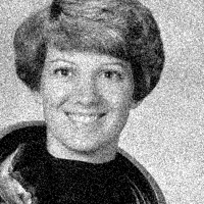
Noisy (σ = 25)Tiny residual CNN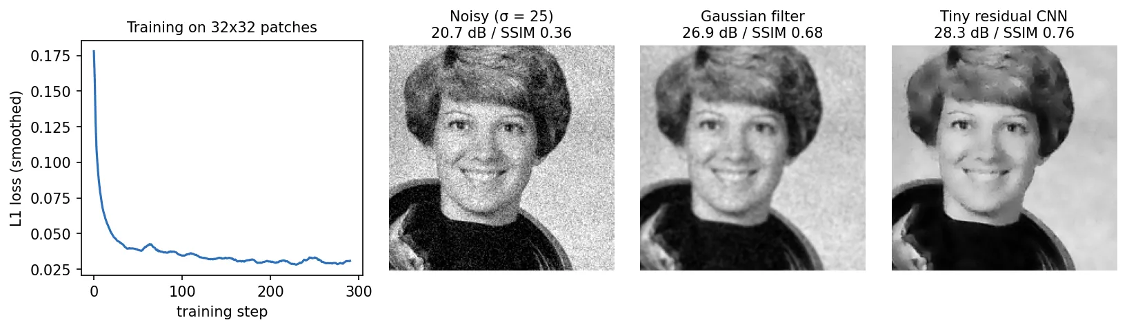

Dehazing

Plain version. Remove the gray-white veil of fog or smog, restoring contrast and color, especially for distant objects. In the post’s words it is an extension of denoising and deblurring, with a physical model attached.

The classical recipe and the dark channel prior

Classical methods estimate the unknowns of $I = J t + A (1 - t)$ (the transmission map $t$ and the airlight $A$), then invert the model. The hard part is finding a reliable relationship that pins those unknowns down. The most famous one is He et al.’s dark channel prior [25]. In haze-free outdoor images, most local patches contain some pixel that is very dark in at least one color channel (shadows, dark or colorful objects):

$$J^{\text{dark}}(p) = \min_{c \in \{r, g, b\}} \Bigl( \min_{q \in \Omega(p)} J^c(q) \Bigr) \approx 0,$$

where $\Omega(p)$ is a small patch around $p$ and $J^c$ is color channel $c$. Applying the same min–min operation to the haze model and using $J^{\text{dark}} \approx 0$ gives a transmission estimate

$$\tilde t(p) = 1 - \omega \min_c \Bigl( \min_{q \in \Omega(p)} \frac{I^c(q)}{A^c} \Bigr),$$

where $\omega \lt 1$ (0.95 in the paper) keeps a little haze for depth perception. Then $\hat J = (I - A)/\max(\tilde t, t_0) + A$, with a small $t_0$ to avoid dividing by zero. The prior fails on large bright regions similar to the airlight (white walls, sky), and the coarse patch-based $t$ must be refined to follow edges.

Deep dehazing: two schools

The post [1] divides deep dehazing into two schools, and the split still describes the field well.

1. Physics-guided (“apply the formula”). Learn the unknown parameters, then invert the model. DehazeNet [26] uses a CNN (with Maxout units and a bounded ReLU) to regress the transmission $t$ from hazy patches. AOD-Net [27] simplifies the scattering model further by folding $t$ and $A$ into a single function $K$:

$$J(p) = K(p)\, I(p) - K(p) + b, \qquad K(p) = \frac{\frac{1}{t(p)}\bigl(I(p) - A\bigr) + (A - b)}{I(p) - 1},$$

where $b$ is a constant bias. A light-weight CNN predicts $K$, so the whole network is end-to-end, and it can be attached in front of a detector and trained jointly.

2. Strong general architectures (“big learner”). Skip the physics and learn $I \mapsto J$ directly with a powerful network. GridDehazeNet [28] uses an attention-based multi-scale grid; FFA-Net [29] stacks channel- and pixel-attention blocks with adaptive feature fusion. These designs transfer well to other degradations, which is exactly the route taken by general restoration networks such as MIRNet [30]. Transformer dehazers followed: DehazeFormer [31] adapts the Swin Transformer to dehazing with a modified normalization layer, activation and spatial aggregation.

Datasets

• RESIDE [32]: a large benchmark with synthetic indoor and outdoor hazy images (generated from depth with the scattering model) plus real hazy images for task-driven evaluation. Its SOTS test set is the most quoted dehazing benchmark.
• O-HAZE [33] and Dense-Haze [34]: real hazy/haze-free pairs captured with professional haze machines, outdoor and with dense haze respectively. They are small but expose the synthetic-to-real gap.
• KITTI [35] is not a dehazing dataset. It is an autonomous-driving benchmark (stereo, optical flow, odometry, 3-D detection, tracking) recorded around Karlsruhe. Some dehazing papers synthesize fog on its images (it has depth from LiDAR and stereo) or use it to measure how dehazing affects downstream detection.

Desnowing

Plain version. Remove falling snow. It looks like a cousin of deraining, but it also behaves like dehazing.

Snow is harder than it looks. Snowflakes vary hugely in size and transparency, from opaque white blobs to semi-transparent streaks, and heavy snow also creates a veiling effect much like haze. So a desnowing model has to handle both the flakes and the fog-like veil. DesnowNet [36] introduced the Snow100K dataset (synthetic snow over real images, plus real snowy images) and a network that estimates both the translucency of snow and the residual it leaves. JSTASR [37] explicitly models snow size and transparency and adds a veiling-effect removal step. Desnowing is now usually studied inside “adverse weather” all-in-one models such as TransWeather [52].

Deraining

Plain version. Remove rain from photos. “Rain” means two very different things: thin streaks falling through the air, and drops sitting on the lens or windshield.

Rain streaks versus raindrops

• Rain streaks are thin, bright, oriented lines overlaid on the scene, modeled as $I = B + R$. Distant streaks accumulate into a haze-like veil. Methods learn to separate the two layers. An early influential deep method jointly detects and removes rain [38] and comes with widely used synthetic datasets of light and heavy rain.
• Raindrops on a glass surface act as tiny lenses: they hide and refract the background, are often out of focus, and have no consistent orientation. The attentive GAN of Qian et al. [39] uses an attention map (where are the drops?) to guide both the generator and the discriminator, and introduced a paired raindrop dataset captured through glass with and without water drops.

Toward real scenes

Most deraining datasets are synthetic, and models trained on synthetic streaks often fail on real rain. The NTIRE 2025 Day and Night Raindrop Removal for Dual-Focused Images challenge [40] reflects the shift to real data: it uses the real-captured Raindrop Clarity dataset, covering daytime and nighttime scenes and both raindrop-focused and background-focused shots (14,139 training, 240 validation and 731 test images). The focus setting matters: when the camera focuses on the drops, the background is blurred too, so raindrop removal becomes partly deblurring.

Low-light enhancement (brief)

Plain version. Make a dark photo look properly exposed, with visible details and natural colors, without blowing up the noise.

Training compares dark images with normally exposed references of the same scene, for example the LOL dataset of paired low/normal-light images introduced with RetinexNet [41]. Classical methods rely on contrast adjustment (histogram equalization) and Retinex-based models (and, less often, an inverted atmospheric scattering model). Deep methods follow two lines: Retinex-inspired networks that decompose $S = R \cdot L$ and adjust $L$ (RetinexNet [41]), and general well-designed networks. Retinexformer [42] (ICCV 2023), which its authors describe as the first Transformer-based low-light enhancement method, combines both: a one-stage Retinex formulation with illumination-guided attention. Low-light enhancement has enough of its own (zero-reference methods, curves, noise, color, video) to deserve a separate chapter: see DL 05.

Image fusion (brief)

Plain version. Combine several images of the same scene, each good at something different, into one image that has the best of each.

Three common settings appear in the post [1]: infrared and visible fusion (thermal targets from IR, textures and color from the visible camera), multi-exposure fusion (detail from under- and over-exposed shots, an HDR-like result) and multi-focus fusion (an all-in-focus image from shots focused at different depths). Unlike the other tasks, there is usually no ground-truth fused image, so deep fusion relies on unsupervised losses that keep gradients and intensities from the sources, or on GANs. The survey by Zhang et al. [43] organizes deep fusion methods by these scenarios and by learning strategy.

Deblurring

Plain version. Recover a sharp image from one smeared by camera shake, object motion or defocus.

Problem setup

Deblurring is the direct instance of $g = h * f + n$. If the kernel $h$ is known it is non-blind deblurring (the setting of the classical Wiener and CLS filters in DIP 5, and of learned non-blind solvers); if $h$ is unknown it is blind deblurring. Real motion blur in dynamic scenes is worse: different objects move differently and depth varies, so there is no single global $h$.

Data and milestones

Nah et al. [44] (CVPR 2017) addressed this with the GoPro dataset: they recorded sharp video with a high-speed camera and averaged consecutive frames to produce realistically blurred images, keeping the middle frame as the sharp target. Their network is multi-scale: it restores a coarse version first, then refines at finer scales, like the coarse-to-fine schemes of classical blind deblurring, but without estimating a kernel at all. GoPro is still the most common deblurring benchmark.

Today the most common baselines are the general backbones Restormer [23] and NAFNet [24]. NAFNet’s striking finding is that the usual nonlinear activations (ReLU, GELU, Sigmoid) are not needed: they can be replaced by a simple element-wise multiplication of two feature halves (“SimpleGate”) or removed, giving a “nonlinear activation free” network that is both simpler and stronger on GoPro and SIDD. The deblurring survey by Zhang et al. [69] covers the wider landscape (blind and non-blind, video, defocus, losses).

Inpainting (brief)

Plain version. Fill in missing or damaged regions (scratches, removed objects, holes) with plausible content.

Inpainting is the restoration task closest to image generation: inside a large hole there is nothing to restore, only something to invent that matches the surroundings. The degradation is a mask, $y = m \odot x$, where $m$ is 0 in the hole and 1 elsewhere. Masked autoencoders (MAE) [45] can be seen as inpainting used as a pre-training task: hide 75% of image patches and train a ViT to reconstruct them, which turns out to teach strong visual representations. For practical inpainting, LaMa [46] uses fast Fourier convolutions with an image-wide receptive field and training on large masks to fill big holes at high resolution; today, diffusion-based inpainting is the default for large, semantic edits.

Matting (brief)

Plain version. Cut out the foreground (a person, their hair) with soft, partially transparent edges so it can be pasted on a new background.

Matting assumes each pixel is a blend of foreground and background,

$$I = \alpha F + (1 - \alpha) B,$$

where $\alpha \in [0, 1]$ is the opacity (alpha matte), $F$ the foreground color and $B$ the background color. With seven unknowns per pixel ($\alpha$ and two RGB colors) and three observations, the problem is badly underdetermined, so classical methods ask the user for a trimap (definite foreground, definite background, unknown band). It can be seen as a soft variant of segmentation. Background Matting [47] replaces the trimap with an extra photo of the background without the subject, and trains networks first on synthetic composites and then on real images with an adversarial loss that judges how natural the new composites look.

General backbones

Plain version. Across all these tasks, a handful of network designs keep winning. They are general “image-to-image engines” that you can train on any of the degradations above.

Backbone	Core idea	Why it suits restoration
U-Net [48]	Encoder–decoder with skip connections at every scale	Large receptive field from the downsampling path, fine detail from the skips
SwinIR [14]	Residual groups of shifted-window self-attention blocks at full resolution	Content-adaptive weights; strong for SR, denoising, JPEG
Restormer [23]	U-Net of transformer blocks; attention computed across channels (transposed attention) plus gated feed-forward	Cost linear in the number of pixels, so it scales to large images
NAFNet [24]	U-Net of simple conv blocks with LayerNorm, SimpleGate and simplified channel attention; no nonlinear activations	Very strong accuracy per FLOP; the default “simple baseline”
MambaIR / MambaIRv2 [49], [50]	Selective state-space (Mamba) scans with local enhancement and channel attention; v2 adds “attentive” non-causal scanning	Global receptive field at linear cost

Design reasons that recur. (1) Global residual: predict $x - y$ (or $x$ minus an upsampled $y$) so the network learns only the missing part. (2) No batch normalization in most SR/restoration nets since EDSR [10]: BN statistics differ between training patches and full test images and hurt color/range fidelity. (3) Large receptive field at manageable cost: multi-scale U-Nets, windowed or channel attention, state-space scans. Restoration needs context (to tell a texture from noise) and full-resolution detail. (4) Attention or gating for content-adaptive processing: channel attention (RCAN), gating (NAFNet, Restormer). The post’s “Extension” list predicted new architectures from ViT, flow, GAN and diffusion; by 2026 the state-space model joined CNNs and transformers as a third backbone option [49], [50].

All-in-one and universal restoration

Plain version. Instead of training one model for rain, another for haze and another for noise, train one model that figures out what is wrong with the image and fixes it.

Motivation

The post’s “Extension” section lists all-in-one restoration as one of the hottest topics of 2023, starting around 2021. The motivation is practical: in a deployed system we do not know in advance which degradation (or mixture) a given image has, and weather can change or combine at any moment. A bank of task-specific models needs a reliable classifier in front and wastes memory; a single model that adapts is more convenient. The difficulty is task interference: different degradations need different, sometimes opposite operations (denoising smooths, deblurring sharpens), so naive multi-task training underperforms specialists.

Representative methods

• AirNet [51] (CVPR 2022), the “airnet” of the original post: a contrastive-learning degradation encoder extracts a representation of how the image is degraded, without labels, and that representation guides the restoration network. It handles unknown corruption types with one model; its noise + rain + haze setting became the standard “three-task” benchmark.
• TransWeather [52] (CVPR 2022): a single transformer encoder–decoder for rain, fog and snow, with learnable weather-type queries in the decoder.
• PromptIR [53] (NeurIPS 2023): a Restormer-style network with lightweight prompt blocks. Learnable prompt components are combined with weights predicted from the input features and injected into the decoder, encoding degradation-specific information. Tested on denoising, deraining and dehazing.
• AdaIR [54] (ICLR 2025): observes that different degradations affect different frequency sub-bands, then mines low- and high-frequency features from the input and modulates them adaptively. Covers five degradations: noise, haze, rain, motion blur and low light.
• DA-CLIP [55] (ICLR 2024): adapts the vision–language model CLIP with a trained controller so that its image encoder yields both a clean-content embedding and a degradation embedding from a corrupted image; these guide a restoration network through cross-attention.
• InstructIR [56] (ECCV 2024): the user writes a natural-language instruction (“remove the rain”, “make it brighter”), a text encoder embeds it, and the embedding modulates the restoration network.

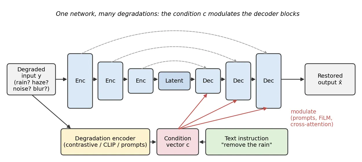
The post’s original motivation is still the core; what changed is who decides the degradation type. It moved from fixed task labels to learned prompts, to vision–language embeddings and finally to human instructions, often backed by large pretrained models. The all-in-one survey [72] discusses this in detail.

Loss functions

Plain version. The loss decides what “good” means. Pixel losses reward being close to the truth on average; perceptual and adversarial losses reward looking real; frequency losses reward getting fine detail.

Pixel losses. With $\hat x = f_\theta(y)$,

$$\ell_2 = \frac{1}{P}\sum_{p} (\hat x_p - x_p)^2, \qquad \ell_1 = \frac{1}{P}\sum_p |\hat x_p - x_p|, \qquad \ell_{\varepsilon} = \frac{1}{P}\sum_p \sqrt{(\hat x_p - x_p)^2 + \varepsilon^2},$$

where $P$ is the number of pixel values and $\varepsilon$ a small constant that makes the last one a smooth, differentiable version of L1. L2 directly optimizes PSNR but penalizes large errors heavily and converges to the posterior mean. Zhao et al. [57] showed that the loss alone changes results noticeably with the architecture fixed, and that L1 and perceptually motivated losses (including combinations with SSIM) often beat L2 even on L2-related metrics. L1 is the default in most modern SR and restoration papers.

Perceptual (feature) loss. Compare images in the feature space of a pretrained classification network $\phi$ (usually VGG) [58]:

$$\ell_{\text{feat}} = \frac{1}{C_j H_j W_j} \bigl\| \phi_j(\hat x) - \phi_j(x) \bigr\|_2^2,$$

where $\phi_j$ is the feature map of layer $j$ with $C_j$ channels and size $H_j \times W_j$. It tolerates small misalignments and rewards matching edges and textures rather than exact values.

Adversarial loss. A discriminator $D_\psi$ learns to tell restored from real images and the restorer learns to fool it, e.g. $\ell_{\text{adv}} = -\log D_\psi(\hat x)$. This pushes outputs onto the manifold of natural images (SRGAN [12], ESRGAN [13], Real-ESRGAN [4]) at the cost of possible hallucinated texture. In practice GAN-based restorers use a weighted sum such as $\ell = \ell_1 + \lambda_p \ell_{\text{feat}} + \lambda_a \ell_{\text{adv}}$ with weights $\lambda_p, \lambda_a$.

Frequency losses. Networks tend to fit low frequencies first and under-fit fine detail. Adding a loss on the Fourier transform $\mathcal F$, such as $\| \mathcal F(\hat x) - \mathcal F(x) \|_1$ on complex values or on amplitude, directly penalizes missing high frequencies. The focal frequency loss [59] goes further and adaptively up-weights the frequency components that are currently hardest to reconstruct. Frequency terms are now common in deblurring and all-in-one models.

Evaluation metrics

Plain version. “Is the restored image close to the truth?” and “Does it look like a real photo?” are different questions, answered by different metrics, and you cannot maximize both at once.

Full-reference metrics

PSNR (peak signal-to-noise ratio):

$$\mathrm{PSNR}(x, \hat x) = 10 \log_{10} \frac{\mathrm{MAX}^2}{\mathrm{MSE}(x, \hat x)},$$

where $\mathrm{MAX}$ is the largest possible pixel value (1 or 255) and $\mathrm{MSE}$ is the mean squared error. It is measured in dB; +1 dB is a 21% reduction in MSE.

SSIM (structural similarity) [60] compares local means, variances and covariance:

$$\mathrm{SSIM}(a, b) = \frac{(2\mu_a \mu_b + C_1)(2\sigma_{ab} + C_2)}{(\mu_a^2 + \mu_b^2 + C_1)(\sigma_a^2 + \sigma_b^2 + C_2)},$$

computed over local windows $a$, $b$ of the two images and averaged, where $\mu$ are local means, $\sigma^2$ local variances, $\sigma_{ab}$ the local covariance and $C_1, C_2$ small constants for stability. It correlates better with perceived structure than PSNR but still prefers smooth results.

LPIPS [61] measures distance between deep-network features (calibrated on human similarity judgments). Lower is better, and it rewards realistic textures that PSNR penalizes.

import numpy as np
from scipy import ndimage as ndi
from skimage import data, img_as_float32
from skimage.metrics import peak_signal_noise_ratio, structural_similarity

x = img_as_float32(data.camera())
y = np.clip(x + np.random.default_rng(0).normal(0, 0.1, x.shape), 0, 1).astype(np.float32)
x_hat = ndi.gaussian_filter(y, 1.0)

def psnr(ref, est, peak=1.0):
    mse = np.mean((ref.astype(np.float64) - est) ** 2)
    return 10 * np.log10(peak ** 2 / mse)

print(f"PSNR  ours {psnr(x, x_hat):.2f} dB | skimage {peak_signal_noise_ratio(x, x_hat, data_range=1):.2f} dB")
print(f"SSIM  {structural_similarity(x, x_hat, data_range=1):.3f}")
# PSNR  ours 27.20 dB | skimage 27.20 dB
# SSIM  0.639

Always report the conventions (RGB or Y channel, border crop, data range, 8-bit rounding): differences in these alone can shift published PSNR by tenths of a dB.

No-reference metrics

When there is no ground truth (real photos), we use no-reference quality measures. NIQE [62] fits a multivariate Gaussian to natural-scene statistics of pristine images and measures how far a test image’s statistics are from it (lower is better, no training on human scores). The Perceptual Index (PI) of the PIRM 2018 challenge [63] combines NIQE with a learned no-reference score into one number. FID [64] compares the distribution of Inception features of a set of outputs with a set of real images; it was designed for generative models and is used for generative restoration such as diffusion SR. IS (Inception Score), mentioned in the post, measures confidence and diversity of class predictions; it is better suited to class-conditional generation than to restoration and is rarely used there today.

The perception–distortion trade-off

Blau and Michaeli [65] formalized the tension. Let $\Delta(x, \hat x)$ be any distortion measure (MSE, $1 -$ SSIM, …) and $d(p_X, p_{\hat X})$ a divergence between the distribution of real images and that of restored images (perceptual quality: small $d$ means outputs are statistically indistinguishable from real images). The perception–distortion function is

$$P(D) = \min_{p_{\hat X \mid Y}} \; d\bigl(p_X,\, p_{\hat X}\bigr) \quad \text{subject to} \quad \mathbb E\bigl[\Delta(X, \hat X)\bigr] \le D,$$

where the minimum is over all (possibly random) restoration methods. They proved that $P(D)$ is non-increasing and (for divergences convex in their second argument) convex: there is an unattainable region near the origin. A method cannot be both minimal-distortion and perfectly realistic. In particular, the MMSE estimator $\mathbb E[x \mid y]$ has the lowest distortion but a blurry, unrealistic output distribution; to look real you must accept higher MSE. GANs (and now diffusion models) are principled ways to move along the bound.

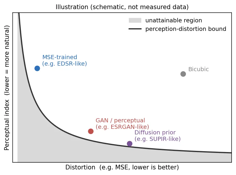
This is the update in the post’s metric section: since diffusion models can generate plausible but unfaithful detail, the gap between fidelity (PSNR/SSIM) and perceptual quality has become central. The NTIRE 2025 $\times 4$ SR challenge therefore ran two tracks: a restoration track ranked by PSNR and a perceptual track ranked by a perceptual score [3], whereas the 2024 edition ranked by PSNR [2]. Practical advice: report both a distortion and a perceptual metric, and say where on the trade-off your method aims.

NTIRE challenges

Plain version. Each year a CVPR workshop runs public competitions on fixed datasets and publishes a report describing the winning ideas: the easiest way to see what currently works.

The NTIRE challenge reports are a good way to follow restoration now that per-task leaderboards are gone. Each report describes the task, data, evaluation protocol and the methods of top teams. Examples cited in this tutorial:

• NTIRE 2017 SR [19]: introduced DIV2K; EDSR [10] won.
• NTIRE 2024 $\times 4$ SR [2]: bicubic $\times 4$ on DIV2K, ranked by PSNR.
• NTIRE 2025 $\times 4$ SR [3]: separate restoration (PSNR) and perceptual tracks.
• NTIRE 2025 raindrop removal [40]: real day and night raindrop images with dual focus.

Two patterns appear across recent reports: winning entries are usually ensembles or large hybrids of the backbones above (HAT-, Restormer-, NAFNet- or Mamba-style, sometimes with diffusion priors) trained with heavy data and compute, and challenges increasingly use real captured data and perceptual tracks.

Modern view

The post closes with an extension list (medical images, multimodal, unsupervised, new architectures, all-in-one, low-level plus high-level, real-time, underwater). Most of these are now active areas. Here we summarize the survey literature task by task, then the 2023–2026 state of the art and the open problems.

Survey papers

• Wang, Chen and Hoi, “Deep Learning for Image Super-resolution: A Survey” (TPAMI 2021) [66]. Organizes SR into supervised, unsupervised and domain-specific SR; within supervised SR it dissects models by upsampling position (pre-, post-, progressive, iterative up-and-down), upsampling operator (interpolation, transposed convolution, sub-pixel), network design (residual, recursive, dense, attention, multi-path), losses and training strategies. Takeaway: most SR progress can be described as choices along these axes, and unsupervised/real-world SR was flagged as the main open direction, which the field then pursued.
• Tian et al., “Deep Learning on Image Denoising: An Overview” (Neural Networks 2020) [67]. Groups CNN denoisers into additive white noise, real noise, blind denoising, and hybrid noise with blur or low resolution, and compares them on public benchmarks. Takeaway: the realism of the noise model, not the network, is often the bottleneck.
• Elad, Kawar and Vaksman, “Image Denoising: The Deep Learning Revolution and Beyond” (SIAM J. Imaging Sciences 2023) [68]. Traces denoising from classical priors to deep networks, then argues that denoisers are now building blocks for other inverse problems (plug-and-play, regularization by denoising) and for diffusion-based image generation, and that restoration should embrace multiple valid solutions (posterior sampling) instead of one answer. Takeaway: the field’s frontier moved from “better MMSE denoisers” to “sampling from the posterior”.
• Zhang et al., “Deep Image Deblurring: A Survey” (IJCV 2022) [69]. Covers causes of blur, datasets and metrics, and a taxonomy of CNN deblurring by architecture, loss and application (faces, text, stereo), for both blind and non-blind settings. Takeaway: dynamic-scene deblurring moved from kernel estimation to end-to-end, multi-scale networks trained on captured pairs such as GoPro.
• Gui et al., “A Comprehensive Survey and Taxonomy on Single Image Dehazing Based on Deep Learning” (ACM Computing Surveys 2023) [70]. Splits methods into supervised, semi-supervised and unsupervised, and within each by whether and how they use the scattering model; also reviews datasets, network modules, losses and metrics, with experiments on baselines. Takeaway: physics-guided and physics-free designs coexist, and the synthetic-to-real gap is the main open problem.
• Yang et al., “Single Image Deraining: From Model-Based to Data-Driven and Beyond” (TPAMI 2021) [71]. Reviews rain appearance models, model-based methods (priors and optimization) and data-driven methods (architectures, constraints, losses, datasets). Takeaway: realistic rain models and real-world evaluation matter more than further architecture tweaks on synthetic data.
• Jiang et al., “A Survey on All-in-One Image Restoration: Taxonomy, Evaluation and Future Trends” (TPAMI, 2025) [72]. Organizes all-in-one methods by architectural design, learning paradigm and core innovation (degradation representations, prompts, mixture-of-experts, language guidance), and consolidates datasets and evaluation protocols. Takeaway: comparisons are complicated by inconsistent task sets, and generalization to unseen and mixed degradations remains open.
• Li et al., “Diffusion Models for Image Restoration and Enhancement: A Comprehensive Survey” (IJCV 2025) [73]. Categorizes diffusion-based restoration by learning paradigm (supervised versus zero-shot use of a pretrained prior), conditioning strategy, framework design and modeling strategy, with focus on SR, deblurring, inpainting and blind/real-world restoration. Takeaway: diffusion gives the best perceptual quality but at high compute cost and with fidelity/hallucination concerns; distillation to few steps and better evaluation are key directions.

State of the art, 2023–2026

1. All-in-one and blind restoration became the mainstream setting, not a niche topic. Methods moved from learned degradation representations (AirNet) to prompts (PromptIR), frequency-aware adaptation (AdaIR) and language guidance (DA-CLIP, InstructIR).
2. Pretrained diffusion models as generative priors transformed real-world SR and blind restoration (DiffBIR, SUPIR), and one-step variants (OSEDiff) cut the inference cost from tens or hundreds of steps to one.
3. State-space models (MambaIR, MambaIRv2) joined CNNs and transformers as backbone options with global receptive fields at linear cost.
4. Evaluation caught up with generation: challenges separate fidelity from perceptual tracks [3], and real captured datasets (SIDD, O-HAZE, Dense-Haze, Raindrop Clarity) are standard alongside synthetic benchmarks.

Open problems

• Real-world generalization. Synthetic pipelines still miss real camera processing, spatially varying blur and mixed weather; models degrade on unseen combinations.
• Fidelity versus hallucination. Generative priors can invent text, faces or textures. For medical, forensic and scientific use this is unacceptable, and we lack good metrics for “faithful but sharp”.
• Evaluation. PSNR/SSIM reward blur; no-reference metrics can be gamed; human studies are costly. Agreement between metrics and human preference for generative restoration is still weak.
• Efficiency. High-resolution, real-time (and video) restoration on phones and cameras remains a strong constraint, for transformers and diffusion models especially.
• Task interference and scaling in all-in-one models, and how to add a new degradation without retraining.
• Low-level plus high-level. Restoration that helps downstream detection or segmentation, rather than human viewers, is a different objective (task-driven evaluation, as in RESIDE [32]).

The author’s perspective

The post ends with two observations that still hold. First, because each task is simple to state, the race for state of the art is largely won by special architectures, which means a lot of compute and complicated experiments; but these tasks are very practical and easy to apply, so there is much room in applications and in combining tasks (exactly where all-in-one restoration went). Second, compared with high-level tasks the learning curve is gentle: a beginner can easily picture what the model is doing (a damaged image goes in, a cleaner one comes out), which makes low-level vision a good door into deep learning research.

Key takeaways

• Low-level vision is about perceiving pixels well; almost every task is an instance of $y = \mathcal D(x) + n$ with a different $\mathcal D$ (blur, downsampling, JPEG, scattering, rain layer, Retinex illumination, mask).
• Deep learning moved the degradation model from the solver into the data generator: realistic, randomized synthetic pipelines (and captured pairs) are as important as the network.
• Upsampling in SR evolved from bicubic pre-upsampling (SRCNN) through transposed convolution (FSRCNN) to sub-pixel convolution (ESPCN), which is the standard today.
• A few general backbones dominate: U-Net-style CNNs (NAFNet), transformers (SwinIR, Restormer, HAT) and state-space models (MambaIR); key design habits are global residuals, no batch norm, large receptive fields and gating/attention.
• All-in-one models (AirNet, TransWeather, PromptIR, AdaIR, DA-CLIP, InstructIR) handle unknown degradations by conditioning one network on a learned, prompted or text-given degradation description.
• L2/L1 losses give faithful but smooth results; perceptual, adversarial and diffusion-based methods give realistic but less faithful ones. The perception–distortion trade-off says you cannot have both at the limit, so report both kinds of metric.
• KITTI is a driving benchmark, not a dehazing dataset; for dehazing use RESIDE plus real pairs such as O-HAZE and Dense-Haze.

Exercises

1. Degradation order. Using the degrade function, compare (a) blur → downsample → noise → JPEG with (b) noise → blur → downsample → JPEG at the same parameters. Visually and with the noise standard deviation measured on a flat patch, explain why the order matters for what the network has to learn.

Hint

In (b), the blur and downsampling filter the noise: its standard deviation drops and it becomes spatially correlated (smooth blotches rather than per-pixel grain). In (a), the noise stays white at the low resolution. A network trained only on (a) will under-remove correlated noise at test time. This is one reason Real-ESRGAN randomizes and repeats the stages.

2. Pixel shuffle by hand. A feature tensor has shape $(C s^2, H, W) = (4, 2, 2)$ with $s = 2$, $C = 1$, and channel $k$ is filled with the constant $k$. Write the $4 \times 4$ output of pixel shuffle using the formula in the SR section, then check with torch.nn.PixelShuffle(2).

Hint

Output pixel $(2h + i, 2w + j)$ takes channel $2i + j$. So every $2 \times 2$ block is $\begin{bmatrix} 0 & 1 \\ 2 & 3 \end{bmatrix}$, and the $4 \times 4$ output repeats that block four times. Each output block gathers one value from each of the four channels at the same low-resolution position.

3. Residual or direct? Modify TinyDnCNN.forward to return self.body(y) (predict the clean image directly) and train both versions with the same seed and steps. Compare PSNR and the loss curves. Then repeat with $\sigma = 5/255$. When does residual learning help most?

Hint

With few training steps, the residual version usually converges faster and reaches a higher PSNR, because at initialization it already outputs roughly $y$ (good PSNR) and only needs to learn a small correction. At low noise the direct version struggles most, since it must learn a near-identity mapping through several ReLU layers.

4. Dark channel by numbers. A hazy pixel has $I = (0.75, 0.78, 0.80)$, the darkest value of $I^c / A^c$ over its patch and channels is $0.70$, and $A = (0.9, 0.9, 0.9)$. With $\omega = 0.95$ and $t_0 = 0.1$, compute $\tilde t$ and the recovered $\hat J$ for this pixel.

Hint

$\tilde t = 1 - 0.95 \times 0.70 = 0.335$. Then $\hat J^c = (I^c - 0.9)/0.335 + 0.9$, giving about $(0.452, 0.542, 0.601)$. The output is darker and more saturated than the input, as expected when the veil is removed.

5. Perception versus distortion. Take the tiny denoiser’s output and add a small amount of fresh Gaussian noise ($\sigma = 3/255$) to it. Compute PSNR and SSIM before and after. The image may look more natural (less plastic) although both metrics drop. Relate this to the perception–distortion function $P(D)$.

Hint

The MMSE-like output lies at low distortion but far from the natural-image distribution (too smooth). Adding grain moves the output distribution closer to real photos (lower $d$) at the price of higher MSE: a move along, or toward, the convex bound, not past it.

6. Design an all-in-one experiment. You must build a single model for noise ($\sigma \in [0, 50]$), rain streaks and haze. Describe the training data mix, how you would condition the network (no labels at test time), the baselines you would compare against, and how you would detect task interference.

Hint

Mix datasets per task with balanced sampling; add a degradation encoder (contrastive as in AirNet, or prompts as in PromptIR) trained jointly. Compare with three single-task models of the same backbone and size, and with a version without conditioning. Interference shows up as the all-in-one model falling behind the single-task model on one task while matching it on others; also test on mixed degradations (rain + haze) unseen in training.

References

1. Shyandram, “Low-Level Vision Task-Image Restoration簡介,” blog post (in Traditional Chinese), 2023; updated 2026. link
2. Z. Chen, Z. Wu, E. Zamfir, K. Zhang, Y. Zhang, R. Timofte et al., “NTIRE 2024 Challenge on Image Super-Resolution (×4): Methods and Results,” in Proc. IEEE/CVF CVPR Workshops, 2024. arXiv
3. Z. Chen, K. Liu, J. Gong, J. Wang, L. Sun et al., “NTIRE 2025 Challenge on Image Super-Resolution (×4): Methods and Results,” in Proc. IEEE/CVF CVPR Workshops, 2025. arXiv
4. X. Wang, L. Xie, C. Dong and Y. Shan, “Real-ESRGAN: Training Real-World Blind Super-Resolution with Pure Synthetic Data,” in Proc. IEEE/CVF ICCV Workshops, 2021. arXiv
5. E. H. Land and J. J. McCann, “Lightness and Retinex Theory,” Journal of the Optical Society of America, vol. 61, no. 1, pp. 1–11, 1971. doi
6. C. Dong, C. C. Loy, K. He and X. Tang, “Image Super-Resolution Using Deep Convolutional Networks,” IEEE TPAMI, 2016 (conference version ECCV 2014). arXiv
7. C. Dong, C. C. Loy and X. Tang, “Accelerating the Super-Resolution Convolutional Neural Network,” in Proc. ECCV, 2016. arXiv
8. W. Shi, J. Caballero, F. Huszár, J. Totz, A. P. Aitken, R. Bishop, D. Rueckert and Z. Wang, “Real-Time Single Image and Video Super-Resolution Using an Efficient Sub-Pixel Convolutional Neural Network,” in Proc. IEEE CVPR, 2016. arXiv
9. A. Odena, V. Dumoulin and C. Olah, “Deconvolution and Checkerboard Artifacts,” Distill, 2016. link
10. B. Lim, S. Son, H. Kim, S. Nah and K. M. Lee, “Enhanced Deep Residual Networks for Single Image Super-Resolution,” in Proc. IEEE CVPR Workshops, 2017. arXiv
11. Y. Zhang, K. Li, K. Li, L. Wang, B. Zhong and Y. Fu, “Image Super-Resolution Using Very Deep Residual Channel Attention Networks,” in Proc. ECCV, 2018. arXiv
12. C. Ledig, L. Theis, F. Huszár, J. Caballero, A. Cunningham, A. Acosta, A. Aitken, A. Tejani, J. Totz, Z. Wang and W. Shi, “Photo-Realistic Single Image Super-Resolution Using a Generative Adversarial Network,” in Proc. IEEE CVPR, 2017. arXiv
13. X. Wang, K. Yu, S. Wu, J. Gu, Y. Liu, C. Dong, C. C. Loy, Y. Qiao and X. Tang, “ESRGAN: Enhanced Super-Resolution Generative Adversarial Networks,” in Proc. ECCV Workshops, 2018. arXiv
14. J. Liang, J. Cao, G. Sun, K. Zhang, L. Van Gool and R. Timofte, “SwinIR: Image Restoration Using Swin Transformer,” in Proc. IEEE/CVF ICCV Workshops, 2021. arXiv
15. X. Chen, X. Wang, J. Zhou, Y. Qiao and C. Dong, “Activating More Pixels in Image Super-Resolution Transformer,” in Proc. IEEE/CVF CVPR, 2023. arXiv
16. X. Lin, J. He, Z. Chen, Z. Lyu, B. Dai, F. Yu, W. Ouyang, Y. Qiao and C. Dong, “DiffBIR: Towards Blind Image Restoration with Generative Diffusion Prior,” arXiv:2308.15070, 2023. arXiv
17. F. Yu, J. Gu, Z. Li, J. Hu, X. Kong, X. Wang, J. He, Y. Qiao and C. Dong, “Scaling Up to Excellence: Practicing Model Scaling for Photo-Realistic Image Restoration In the Wild,” in Proc. IEEE/CVF CVPR, 2024. arXiv
18. R. Wu, L. Sun, Z. Ma and L. Zhang, “One-Step Effective Diffusion Network for Real-World Image Super-Resolution,” in Proc. NeurIPS, 2024. arXiv
19. E. Agustsson and R. Timofte, “NTIRE 2017 Challenge on Single Image Super-Resolution: Dataset and Study,” in Proc. IEEE CVPR Workshops, 2017. doi
20. K. Zhang, W. Zuo, Y. Chen, D. Meng and L. Zhang, “Beyond a Gaussian Denoiser: Residual Learning of Deep CNN for Image Denoising,” IEEE Transactions on Image Processing, vol. 26, no. 7, pp. 3142–3155, 2017. arXiv
21. K. Zhang, W. Zuo and L. Zhang, “FFDNet: Toward a Fast and Flexible Solution for CNN-Based Image Denoising,” IEEE Transactions on Image Processing, 2018. arXiv
22. A. Abdelhamed, S. Lin and M. S. Brown, “A High-Quality Denoising Dataset for Smartphone Cameras,” in Proc. IEEE/CVF CVPR, 2018. doi
23. S. W. Zamir, A. Arora, S. Khan, M. Hayat, F. S. Khan and M.-H. Yang, “Restormer: Efficient Transformer for High-Resolution Image Restoration,” in Proc. IEEE/CVF CVPR, 2022. arXiv
24. L. Chen, X. Chu, X. Zhang and J. Sun, “Simple Baselines for Image Restoration,” in Proc. ECCV, 2022. arXiv
25. K. He, J. Sun and X. Tang, “Single Image Haze Removal Using Dark Channel Prior,” in Proc. IEEE CVPR, 2009. doi
26. B. Cai, X. Xu, K. Jia, C. Qing and D. Tao, “DehazeNet: An End-to-End System for Single Image Haze Removal,” IEEE Transactions on Image Processing, 2016. arXiv
27. B. Li, X. Peng, Z. Wang, J. Xu and D. Feng, “AOD-Net: All-in-One Dehazing Network,” in Proc. IEEE ICCV, 2017. doi · arXiv
28. X. Liu, Y. Ma, Z. Shi and J. Chen, “GridDehazeNet: Attention-Based Multi-Scale Network for Image Dehazing,” in Proc. IEEE/CVF ICCV, 2019. arXiv
29. X. Qin, Z. Wang, Y. Bai, X. Xie and H. Jia, “FFA-Net: Feature Fusion Attention Network for Single Image Dehazing,” in Proc. AAAI, 2020. arXiv
30. S. W. Zamir, A. Arora, S. Khan, M. Hayat, F. S. Khan, M.-H. Yang and L. Shao, “Learning Enriched Features for Real Image Restoration and Enhancement,” in Proc. ECCV, 2020. arXiv
31. Y. Song, Z. He, H. Qian and X. Du, “Vision Transformers for Single Image Dehazing,” IEEE Transactions on Image Processing, vol. 32, 2023. arXiv
32. B. Li, W. Ren, D. Fu, D. Tao, D. Feng, W. Zeng and Z. Wang, “Benchmarking Single-Image Dehazing and Beyond,” IEEE Transactions on Image Processing, 2019. arXiv
33. C. O. Ancuti, C. Ancuti, R. Timofte and C. De Vleeschouwer, “O-HAZE: A Dehazing Benchmark with Real Hazy and Haze-Free Outdoor Images,” in Proc. IEEE/CVF CVPR Workshops, 2018. doi
34. C. O. Ancuti, C. Ancuti, M. Sbert and R. Timofte, “Dense-Haze: A Benchmark for Image Dehazing with Dense-Haze and Haze-Free Images,” in Proc. IEEE ICIP, 2019. doi
35. A. Geiger, P. Lenz and R. Urtasun, “Are We Ready for Autonomous Driving? The KITTI Vision Benchmark Suite,” in Proc. IEEE CVPR, 2012. project page
36. Y.-F. Liu, D.-W. Jaw, S.-C. Huang and J.-N. Hwang, “DesnowNet: Context-Aware Deep Network for Snow Removal,” IEEE Transactions on Image Processing, 2018. arXiv
37. W.-T. Chen, H.-Y. Fang, J.-J. Ding, C.-C. Tsai and S.-Y. Kuo, “JSTASR: Joint Size and Transparency-Aware Snow Removal Algorithm Based on Modified Partial Convolution and Veiling Effect Removal,” in Proc. ECCV, 2020. doi
38. W. Yang, R. T. Tan, J. Feng, J. Liu, Z. Guo and S. Yan, “Deep Joint Rain Detection and Removal from a Single Image,” in Proc. IEEE CVPR, 2017. arXiv
39. R. Qian, R. T. Tan, W. Yang, J. Su and J. Liu, “Attentive Generative Adversarial Network for Raindrop Removal from a Single Image,” in Proc. IEEE/CVF CVPR, 2018. arXiv
40. X. Li, Y. Jin, X. Jin, Z. Wu, B. Li, Y. Wang et al., “NTIRE 2025 Challenge on Day and Night Raindrop Removal for Dual-Focused Images: Methods and Results,” in Proc. IEEE/CVF CVPR Workshops, 2025. arXiv
41. C. Wei, W. Wang, W. Yang and J. Liu, “Deep Retinex Decomposition for Low-Light Enhancement,” in Proc. BMVC, 2018. arXiv
42. Y. Cai, H. Bian, J. Lin, H. Wang, R. Timofte and Y. Zhang, “Retinexformer: One-stage Retinex-based Transformer for Low-light Image Enhancement,” in Proc. IEEE/CVF ICCV, 2023. arXiv
43. H. Zhang, H. Xu, X. Tian, J. Jiang and J. Ma, “Image Fusion Meets Deep Learning: A Survey and Perspective,” Information Fusion, vol. 76, pp. 323–336, 2021. doi
44. S. Nah, T. H. Kim and K. M. Lee, “Deep Multi-scale Convolutional Neural Network for Dynamic Scene Deblurring,” in Proc. IEEE CVPR, 2017. doi · arXiv
45. K. He, X. Chen, S. Xie, Y. Li, P. Dollár and R. Girshick, “Masked Autoencoders Are Scalable Vision Learners,” in Proc. IEEE/CVF CVPR, 2022. arXiv
46. R. Suvorov, E. Logacheva, A. Mashikhin, A. Remizova, A. Ashukha, A. Silvestrov, N. Kong, H. Goka, K. Park and V. Lempitsky, “Resolution-robust Large Mask Inpainting with Fourier Convolutions,” in Proc. IEEE/CVF WACV, 2022. arXiv
47. S. Sengupta, V. Jayaram, B. Curless, S. Seitz and I. Kemelmacher-Shlizerman, “Background Matting: The World is Your Green Screen,” in Proc. IEEE/CVF CVPR, 2020. arXiv
48. O. Ronneberger, P. Fischer and T. Brox, “U-Net: Convolutional Networks for Biomedical Image Segmentation,” in Proc. MICCAI, 2015. arXiv
49. H. Guo, J. Li, T. Dai, Z. Ouyang, X. Ren and S.-T. Xia, “MambaIR: A Simple Baseline for Image Restoration with State-Space Model,” in Proc. ECCV, 2024. arXiv
50. H. Guo, Y. Guo, Y. Zha, Y. Zhang, W. Li, T. Dai, S.-T. Xia and Y. Li, “MambaIRv2: Attentive State Space Restoration,” in Proc. IEEE/CVF CVPR, 2025. arXiv
51. B. Li, X. Liu, P. Hu, Z. Wu, J. Lv and X. Peng, “All-In-One Image Restoration for Unknown Corruption,” in Proc. IEEE/CVF CVPR, 2022. code & paper
52. J. M. J. Valanarasu, R. Yasarla and V. M. Patel, “TransWeather: Transformer-based Restoration of Images Degraded by Adverse Weather Conditions,” in Proc. IEEE/CVF CVPR, 2022. arXiv
53. V. Potlapalli, S. W. Zamir, S. Khan and F. S. Khan, “PromptIR: Prompting for All-in-One Image Restoration,” in Proc. NeurIPS, 2023. arXiv
54. Y. Cui, S. W. Zamir, S. Khan, A. Knoll, M. Shah and F. S. Khan, “AdaIR: Adaptive All-in-One Image Restoration via Frequency Mining and Modulation,” in Proc. ICLR, 2025. arXiv
55. Z. Luo, F. K. Gustafsson, Z. Zhao, J. Sjölund and T. B. Schön, “Controlling Vision-Language Models for Multi-Task Image Restoration,” in Proc. ICLR, 2024. arXiv
56. M. V. Conde, G. Geigle and R. Timofte, “InstructIR: High-Quality Image Restoration Following Human Instructions,” in Proc. ECCV, 2024. arXiv
57. H. Zhao, O. Gallo, I. Frosio and J. Kautz, “Loss Functions for Image Restoration with Neural Networks,” IEEE Transactions on Computational Imaging, 2017 (arXiv title: “Loss Functions for Neural Networks for Image Processing”). arXiv
58. J. Johnson, A. Alahi and L. Fei-Fei, “Perceptual Losses for Real-Time Style Transfer and Super-Resolution,” in Proc. ECCV, 2016. doi · arXiv
59. L. Jiang, B. Dai, W. Wu and C. C. Loy, “Focal Frequency Loss for Image Reconstruction and Synthesis,” in Proc. IEEE/CVF ICCV, 2021. arXiv
60. Z. Wang, A. C. Bovik, H. R. Sheikh and E. P. Simoncelli, “Image Quality Assessment: From Error Visibility to Structural Similarity,” IEEE Transactions on Image Processing, vol. 13, no. 4, pp. 600–612, 2004. doi
61. R. Zhang, P. Isola, A. A. Efros, E. Shechtman and O. Wang, “The Unreasonable Effectiveness of Deep Features as a Perceptual Metric,” in Proc. IEEE/CVF CVPR, 2018. arXiv
62. A. Mittal, R. Soundararajan and A. C. Bovik, “Making a ‘Completely Blind’ Image Quality Analyzer,” IEEE Signal Processing Letters, 2013. doi
63. Y. Blau, R. Mechrez, R. Timofte, T. Michaeli and L. Zelnik-Manor, “The 2018 PIRM Challenge on Perceptual Image Super-resolution,” in Proc. ECCV Workshops, 2018. arXiv
64. M. Heusel, H. Ramsauer, T. Unterthiner, B. Nessler and S. Hochreiter, “GANs Trained by a Two Time-Scale Update Rule Converge to a Local Nash Equilibrium,” in Proc. NeurIPS, 2017. arXiv
65. Y. Blau and T. Michaeli, “The Perception-Distortion Tradeoff,” in Proc. IEEE/CVF CVPR, 2018. arXiv
66. Z. Wang, J. Chen and S. C. H. Hoi, “Deep Learning for Image Super-Resolution: A Survey,” IEEE TPAMI, 2021. arXiv
67. C. Tian, L. Fei, W. Zheng, Y. Xu, W. Zuo and C.-W. Lin, “Deep Learning on Image Denoising: An Overview,” Neural Networks, vol. 131, pp. 251–275, 2020. arXiv
68. M. Elad, B. Kawar and G. Vaksman, “Image Denoising: The Deep Learning Revolution and Beyond — A Survey Paper,” SIAM Journal on Imaging Sciences, vol. 16, no. 3, pp. 1594–1654, 2023. doi · arXiv
69. K. Zhang, W. Ren, W. Luo, W.-S. Lai, B. Stenger, M.-H. Yang and H. Li, “Deep Image Deblurring: A Survey,” International Journal of Computer Vision, 2022. arXiv
70. J. Gui, X. Cong, Y. Cao, W. Ren, J. Zhang, J. Zhang, J. Cao and D. Tao, “A Comprehensive Survey and Taxonomy on Single Image Dehazing Based on Deep Learning,” ACM Computing Surveys, 2023. doi · arXiv
71. W. Yang, R. T. Tan, S. Wang, Y. Fang and J. Liu, “Single Image Deraining: From Model-Based to Data-Driven and Beyond,” IEEE TPAMI, 2021. doi · arXiv
72. J. Jiang, Z. Zuo, G. Wu, K. Jiang and X. Liu, “A Survey on All-in-One Image Restoration: Taxonomy, Evaluation and Future Trends,” IEEE TPAMI, 2025. arXiv
73. X. Li, Y. Ren, X. Jin, C. Lan, X. Wang, W. Zeng, X. Wang and Z. Chen, “Diffusion Models for Image Restoration and Enhancement: A Comprehensive Survey,” International Journal of Computer Vision, 2025. arXiv