ML 02 · Neural Networks from Perceptron to Deep Networks

What you’ll learn

• What a perceptron is, how its learning rule works, and exactly how it differs from logistic regression.
• How stacking layers gives a multilayer perceptron (MLP), what the universal approximation theorem does and does not promise, and what “deep” really means.
• The activation functions in use today (sigmoid, tanh, softmax, ReLU, Leaky ReLU, GELU, SiLU/Swish, SwiGLU) and the normalization layers (BatchNorm, LayerNorm, RMSNorm), with their formulas and derivatives.
• How to pair the output layer with the right loss, and how backpropagation computes every gradient, derived by hand for a two-layer network and checked numerically in NumPy.
• How to train in practice: initialization, SGD, momentum, Adam and AdamW, learning-rate schedules, batch size, gradient clipping, and how to read a loss curve.
• How to diagnose underfitting and overfitting, the regularization tools that fix overfitting, and how residual connections lead to the Transformer.

The big picture

A neural network is a function with many adjustable knobs (its parameters). It takes an input, such as the pixels of an image or two coordinates of a point, and produces an output, such as a class label. Training means turning the knobs, a tiny amount at a time, so the outputs on known examples get closer to the right answers. Everything in this tutorial is about one of three questions: what shape the function has (the architecture), how to measure “closer” (the loss), and how to turn the knobs well (the optimization).

Why it matters: almost every modern system in vision, speech and language is built from the pieces in this tutorial. Convolutional networks, Transformers and diffusion models all use the same ingredients: linear layers, nonlinear activations, normalization, residual connections, a loss, backpropagation and an adaptive optimizer. Once these are clear, the deep-learning track is about arranging them for images.

The perceptron

Plain version. A perceptron is the simplest artificial neuron. It multiplies each input by a weight, adds them up with a bias, and answers “yes” if the total is positive and “no” otherwise. It learns by nudging its weights only when it gets an example wrong.

The model

Rosenblatt introduced the perceptron in 1958 as a model of how a brain might store and recognize patterns [4]. For an input vector $\mathbf{x} \in \mathbb{R}^d$ it computes

$$z = \mathbf{w}^\top \mathbf{x} + b, \qquad \hat{y} = \mathbf{1}[z > 0],$$

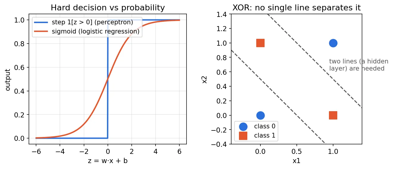
where $\mathbf{w} \in \mathbb{R}^d$ is the weight vector, $b \in \mathbb{R}$ is the bias, $z$ is the pre-activation (a weighted sum), $\mathbf{1}[\cdot]$ is the indicator that equals 1 when its condition is true and 0 otherwise, and $\hat{y} \in \{0, 1\}$ is the predicted class. The indicator is the step function. Geometrically, $\mathbf{w}^\top \mathbf{x} + b = 0$ is a hyperplane (a line in 2-D), and the perceptron labels points by which side of it they fall on.

The perceptron learning rule

Go through the training examples $(\mathbf{x}_i, y_i)$ one at a time. For each one, compute $\hat{y}_i$ and update

$$\mathbf{w} \leftarrow \mathbf{w} + \eta\,(y_i - \hat{y}_i)\,\mathbf{x}_i, \qquad b \leftarrow b + \eta\,(y_i - \hat{y}_i),$$

where $\eta > 0$ is the learning rate (step size) and $y_i \in \{0,1\}$ is the true label. If the prediction is right, $y_i - \hat{y}_i = 0$ and nothing changes. If the perceptron said 0 but the answer was 1, the weights move toward $\mathbf{x}_i$, which raises $z$ for this input next time; the opposite mistake moves them away. When the two classes can be separated by a hyperplane (the data are linearly separable), this rule stops making mistakes after a finite number of updates. When they cannot, it never settles.

import numpy as np

def perceptron_train(X, y, epochs=20, eta=1.0):
    """X: (N, d), y in {0, 1}. Returns w, b."""
    w, b = np.zeros(X.shape[1]), 0.0
    for _ in range(epochs):
        mistakes = 0
        for x_i, y_i in zip(X, y):
            y_hat = float(w @ x_i + b > 0)       # step function
            if y_hat != y_i:                     # update only on a mistake
                w += eta * (y_i - y_hat) * x_i
                b += eta * (y_i - y_hat)
                mistakes += 1
        if mistakes == 0:
            break
    return w, b

# AND is linearly separable; XOR is not
X = np.array([[0, 0], [0, 1], [1, 0], [1, 1]], dtype=float)
for name, y in [("AND", [0, 0, 0, 1]), ("XOR", [0, 1, 1, 0])]:
    w, b = perceptron_train(X, np.array(y, float))
    print(name, (X @ w + b > 0).astype(int))
# AND [0 0 0 1]
# XOR [1 1 0 0]   <- wrong: no single line can do it

Perceptron versus logistic regression

The two models are easy to confuse because they share the same first step, $z = \mathbf{w}^\top\mathbf{x} + b$. They are different methods:

	Perceptron	Logistic regression
Output function	step: $\hat{y} = \mathbf{1}[z > 0]$	sigmoid: $\hat{p} = \sigma(z) = \dfrac{1}{1 + e^{-z}}$
Output meaning	a hard 0/1 decision	a probability $P(y = 1 \mid \mathbf{x})$
Training	perceptron rule, updates only on mistakes	minimize cross-entropy (maximum likelihood) with gradient descent
Non-separable data	never converges	converges to a well-defined best fit

The gradient of the logistic-regression loss for one example is $(\hat{p}_i - y_i)\,\mathbf{x}_i$, so its gradient-descent step is $\mathbf{w} \leftarrow \mathbf{w} + \eta\,(y_i - \hat{p}_i)\,\mathbf{x}_i$. It looks almost identical to the perceptron rule, but $\hat{p}_i$ is a probability between 0 and 1, so every example contributes, and confidently correct ones contribute very little. That smoothness is what makes logistic regression trainable by gradient descent and what lets it be stacked into larger differentiable networks. The step function, in contrast, has derivative zero almost everywhere, so gradients cannot flow through it.

The multilayer perceptron (MLP)

Plain version. One neuron draws one straight line. Put many neurons side by side to get many lines, then feed their outputs into another layer that combines them. The combination can bend, so the network can carve out curved regions.

Stacking layers

An MLP with one hidden layer computes

$$\begin{aligned} \mathbf{h} &= f\!\left(W_1 \mathbf{x} + \mathbf{b}_1\right), \\ \hat{\mathbf{y}} &= g\!\left(W_2 \mathbf{h} + \mathbf{b}_2\right), \end{aligned}$$

where $\mathbf{x} \in \mathbb{R}^d$ is the input, $W_1 \in \mathbb{R}^{m \times d}$ and $\mathbf{b}_1 \in \mathbb{R}^m$ are the first layer’s weights and biases, $m$ is the width (number of hidden units), $f$ is a nonlinear activation function applied element-wise, $\mathbf{h} \in \mathbb{R}^m$ is the hidden representation, $W_2 \in \mathbb{R}^{K \times m}$ and $\mathbf{b}_2 \in \mathbb{R}^K$ map it to $K$ outputs, and $g$ is the output function chosen for the task (see below). Each hidden unit is one “logistic-regression-like” neuron; the name multilayer perceptron is historical, since modern MLPs use smooth activations, not the step function.

The nonlinearity $f$ is essential. Without it, $W_2(W_1\mathbf{x} + \mathbf{b}_1) + \mathbf{b}_2 = (W_2W_1)\mathbf{x} + (W_2\mathbf{b}_1 + \mathbf{b}_2)$ is again a single linear map: any number of linear layers collapses to one, and the network can still only draw one hyperplane. For XOR, two hidden units can each draw one of the dashed lines in Figure 1, and the output unit then answers “between the two lines”.

Universal approximation

Cybenko proved in 1989 that a network with one hidden layer of sigmoidal units can approximate any continuous function on a bounded box (the unit hypercube) to any desired accuracy, provided the hidden layer is wide enough [5]. Later work extended the result to other activations, including ReLU. The theorem is reassuring, but read it carefully:

• It is about existence. It says suitable weights exist; it says nothing about whether gradient descent will find them.
• It says nothing about how wide “wide enough” is. For some functions the required width grows extremely fast with the input dimension.
• It says nothing about generalization: fitting the training points well does not mean predicting new points well.

So the theorem explains why MLPs are flexible enough in principle. The rest of this tutorial is about the practical questions it leaves open.

Deep neural networks: depth and width

Plain version. “Deep” just means many layers stacked in sequence. There is no official number of layers at which a network becomes deep.

A deep neural network (DNN) is an MLP, or any other layered network, with several hidden layers: $\mathbf{h}_\ell = f(W_\ell \mathbf{h}_{\ell-1} + \mathbf{b}_\ell)$ for $\ell = 1, \dots, L$, with $\mathbf{h}_0 = \mathbf{x}$. There is no agreed threshold for “deep”. A common informal usage calls any network with more than one hidden layer deep, while other texts count total layers or hidden layers differently, so “three layers” means different things in different books. What matters is the idea, not the count: a deep network builds its answer as a composition of many simple steps.

The two ways to add capacity are width (more units per layer) and depth (more layers). They are not equivalent. A wider layer adds more pieces that are combined once; a deeper network re-uses the features of earlier layers to build more abstract ones. The review by LeCun, Bengio and Hinton [2] explains the success of deep learning through exactly this point: each layer turns the representation from the previous layer into a slightly more abstract one, and composing many such layers lets the network learn very intricate functions from raw data, with the features learned rather than hand-designed.

Historically, the 1990s were dominated by shallow methods. Support vector machines, a kernel method rather than a wide neural network, were the main tool, and deep networks were hard to train. From the mid-2000s onward, more data, GPUs and better training techniques made depth practical, and deep networks began to win benchmark after benchmark [2]. Depth alone is not the whole story, though: simply stacking more plain layers eventually makes training worse, a problem that residual connections solved (see the last main section).

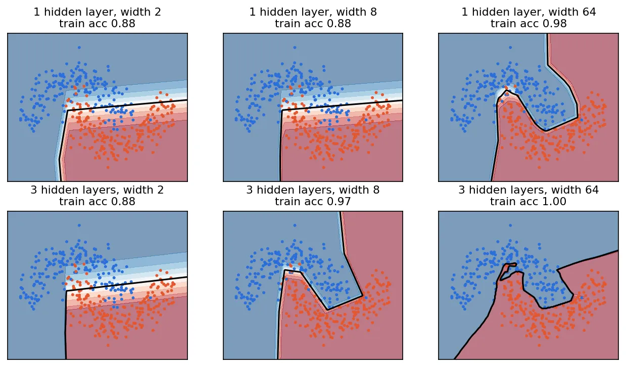
Figure 2 shows width and depth at work on the two-moons dataset from scikit-learn. With two or eight hidden units in one layer, the boundary is made of only a few straight pieces and cannot follow the moons. Wider or deeper networks bend the boundary to fit; the widest and deepest one even wraps around single noisy points, a first hint of overfitting.

Activation functions

Plain version. The activation function is the “bend” applied after each weighted sum. Without it, the whole network would be a straight-line model. Different bends trade off smoothness, speed and how well gradients pass through many layers.

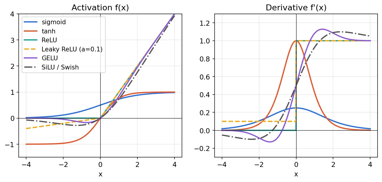
Figure 3 plots the common choices and their derivatives. The derivative matters as much as the function, because backpropagation multiplies derivatives layer after layer (see the training section).

Sigmoid and tanh

$$\sigma(x) = \frac{1}{1 + e^{-x}}, \quad \sigma'(x) = \sigma(x)\big(1 - \sigma(x)\big); \qquad \tanh(x) = 2\sigma(2x) - 1, \quad \tanh'(x) = 1 - \tanh^2(x).$$

The sigmoid maps any real number to $(0, 1)$; tanh maps it to $(-1, 1)$ and is centered at zero. Both saturate: for large $|x|$ the curve is flat and the derivative is nearly zero, so almost no gradient passes through. The sigmoid’s derivative is at most $1/4$ (at $x = 0$). These two facts made deep sigmoid networks hard to train, which Glorot and Bengio analyzed in detail [17]. Today sigmoid is used mainly at the output of binary classifiers and inside gates (as in SwiGLU below), and tanh in some recurrent networks.

Softmax

Softmax turns a vector of $K$ real scores $\mathbf{z}$ (called logits) into a probability distribution:

$$p_k = \operatorname{softmax}(\mathbf{z})_k = \frac{e^{z_k}}{\sum_{j=1}^{K} e^{z_j}}, \qquad \frac{\partial p_k}{\partial z_j} = p_k\big(\delta_{kj} - p_j\big),$$

where $\delta_{kj}$ is 1 if $k = j$ and 0 otherwise. Each $p_k$ is positive and they sum to 1. Unlike the others in this section, softmax acts on a whole vector, not element by element, so it is used almost only in the output layer of multi-class classifiers (and inside attention), not as a hidden activation. In code, subtract $\max_j z_j$ before exponentiating; it does not change the result and avoids overflow.

ReLU and Leaky ReLU

$$\operatorname{ReLU}(x) = \max(0, x), \quad \operatorname{ReLU}'(x) = \mathbf{1}[x > 0]; \qquad \operatorname{LeakyReLU}_a(x) = \max(ax, x), \quad 0 \lt a \lt 1 .$$

The rectified linear unit passes positive inputs unchanged and zeroes the rest. Its derivative is exactly 1 for all positive inputs, so gradients do not shrink as they pass through active units, and it is very cheap to compute. ReLU was one of the changes that made deep supervised networks trainable without unsupervised pre-training [2]. Its weakness is the dying ReLU: a unit whose input is negative for every example has zero gradient and stops learning. Leaky ReLU keeps a small slope $a$ (for example 0.01) on the negative side so some gradient always flows. The activation survey by Dubey, Singh and Chaudhuri [7] groups these and many later variants into a ReLU-based family.

GELU and SiLU/Swish

These are smooth versions of ReLU that let small negative values through:

$$\operatorname{GELU}(x) = x\,\Phi(x), \qquad \operatorname{GELU}'(x) = \Phi(x) + x\,\varphi(x),$$

where $\Phi$ is the standard normal cumulative distribution function and $\varphi$ its density [8]. Instead of gating by sign as ReLU does, GELU weights the input by how large it is: $\Phi(x)$ is the probability that a standard normal variable is below $x$. A common fast approximation is $0.5x\big(1 + \tanh\big[\sqrt{2/\pi}\,(x + 0.044715x^3)\big]\big)$ [8]. GELU is the default activation in many Transformer models.

$$\operatorname{Swish}_\beta(x) = x\,\sigma(\beta x), \qquad \operatorname{SiLU}(x) = x\,\sigma(x), \qquad \operatorname{SiLU}'(x) = \sigma(x)\big(1 + x(1 - \sigma(x))\big).$$

The sigmoid-weighted linear unit (SiLU) was proposed by Elfwing, Uchibe and Doya for reinforcement learning [9]. Ramachandran, Zoph and Le found the same shape with a learnable or fixed $\beta$ by automated search and called it Swish [10]; with $\beta = 1$, Swish is SiLU. GELU and SiLU look very similar (Figure 3). Both are non-monotonic: they dip slightly below zero for moderate negative inputs.

SwiGLU: a gated feed-forward block

A gated linear unit (GLU) multiplies two linear projections element-wise, one of them passed through a nonlinearity that acts like a gate. Shazeer tested several variants in the Transformer’s feed-forward block [11]. The SwiGLU version, written in the paper’s row-vector notation and without biases, is

$$\operatorname{FFN}_{\text{SwiGLU}}(\mathbf{x}) = \big(\operatorname{Swish}_1(\mathbf{x}W) \odot \mathbf{x}V\big)\,W_2,$$

where $\mathbf{x}$ is a row vector of size $d_{\text{model}}$, $W$ and $V$ are $d_{\text{model}} \times d_{\text{ff}}$ matrices, $W_2$ is $d_{\text{ff}} \times d_{\text{model}}$, and $\odot$ is element-wise multiplication. In Shazeer’s experiments the GLU variants, SwiGLU and GEGLU among them, gave better results than the ReLU and GELU versions of the block. Because SwiGLU has three weight matrices instead of two, $d_{\text{ff}}$ is reduced by a factor of $2/3$ to keep the parameter count equal [11]. LLaMA, for example, replaced ReLU with SwiGLU using a hidden size of $\tfrac{2}{3}\cdot 4d$ [12], and SwiGLU has become a common default in large language models.

Activation	Range	Smooth	Typical use today
sigmoid	$(0, 1)$	yes	binary / multi-label output, gates
tanh	$(-1, 1)$	yes	some recurrent networks
softmax	probability vector	yes	multi-class output, attention weights
ReLU / Leaky ReLU	$[0, \infty)$ / $\mathbb{R}$	no (kink at 0)	CNNs, MLPs, the safe default
GELU, SiLU	about $[-0.17, \infty)$, $[-0.28, \infty)$	yes	Transformers, modern CNNs
SwiGLU	$\mathbb{R}$	yes	Transformer feed-forward blocks

Normalization layers

Plain version. As training goes on, the numbers flowing through a network can drift to very large or very small scales, which makes learning unstable. A normalization layer rescales them to a standard size at each step, then lets the network choose the final scale it prefers.

All three common layers share one template. For a set of values $x_1, \dots, x_n$,

$$\mu = \frac{1}{n}\sum_{i=1}^n x_i, \qquad \sigma^2 = \frac{1}{n}\sum_{i=1}^n (x_i - \mu)^2, \qquad y_i = \gamma\,\frac{x_i - \mu}{\sqrt{\sigma^2 + \epsilon}} + \beta,$$

where $\mu$ and $\sigma^2$ are the mean and variance, $\epsilon$ is a small constant for numerical safety, and $\gamma, \beta$ are a learnable scale and shift (so the layer can undo the normalization if that helps). The layers differ in which values form the set (Figure 4).

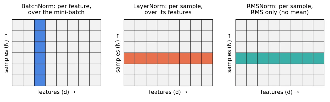
• BatchNorm (Ioffe and Szegedy [13]) computes $\mu, \sigma^2$ for each feature (each channel, in a CNN) across the mini-batch. It speeds up training and became standard in CNNs. Because the statistics depend on the batch, it behaves differently in training and inference: at inference it uses running averages collected during training. It also degrades when batches are very small, since the batch statistics become noisy.
• LayerNorm (Ba, Kiros and Hinton [14]) computes $\mu, \sigma^2$ over the features of a single sample. It does not depend on the batch, behaves identically at training and test time, and works naturally for sequences. It is the standard normalization in Transformers.
• RMSNorm (Zhang and Sennrich [15]) drops the mean subtraction and divides by the root mean square, $y_i = \gamma_i\, x_i / \sqrt{\tfrac{1}{n}\sum_j x_j^2 + \epsilon}$. The authors hypothesize that LayerNorm’s re-centering is dispensable and report comparable quality with lower running time [15]. LLaMA uses RMSNorm and applies it to the input of each Transformer sub-layer (“pre-normalization”) rather than to its output [12].

import torch

x = torch.randn(4, 8) * 5 + 3                       # 4 samples, 8 features
ln = torch.nn.LayerNorm(8, elementwise_affine=False)
bn = torch.nn.BatchNorm1d(8, affine=False)
rms = x / torch.sqrt(x.pow(2).mean(dim=1, keepdim=True) + 1e-6)

print(ln(x).mean(dim=1))     # ~0 for every sample (row)
print(bn(x).mean(dim=0))     # ~0 for every feature (column), in train mode
print(rms.pow(2).mean(dim=1))  # ~1 for every sample: unit RMS, mean not removed

Huang et al. [16] survey this family and decompose any normalization method into three choices: which values are pooled together (the normalization area), what operation is applied (standardizing, centering, scaling or whitening), and how the representation is recovered afterward (the learnable affine step). BatchNorm, LayerNorm and RMSNorm differ mainly in the first two.

Designing the output layer and choosing the loss

Plain version. The last layer must speak the language of the answer: any real number for a quantity, a probability for yes/no, a probability distribution for “which of $K$”. Each kind of output has a natural loss, and the pairs below are the ones to use.

Task	Output layer	Output range	Loss
Regression	linear (no activation)	$\mathbb{R}$	mean squared error (MSE, L2) or mean absolute error (MAE, L1)
Binary classification	1 unit + sigmoid	$(0, 1)$	binary cross-entropy
Multi-label (several yes/no)	$K$ units + sigmoid each	$(0,1)^K$	binary cross-entropy per label
Multi-class (exactly one of $K$)	$K$ units + softmax	probability vector	cross-entropy

A common mistake is to put a sigmoid on a regression output. The sigmoid’s range is the open interval $(0, 1)$, and its job is to output a probability for binary or multi-label classification. A regression head is normally linear, so it can produce any real value. A sigmoid on a regression output is reasonable only when the target itself is known to lie between 0 and 1, such as a normalized pixel intensity or a fraction.

The losses, for one example, are

$$\begin{aligned} \text{MSE:}\quad & \ell = \tfrac{1}{2}\lVert \hat{\mathbf{y}} - \mathbf{y} \rVert^2, \\ \text{binary cross-entropy:}\quad & \ell = -\big[\,y \log \hat{p} + (1 - y)\log(1 - \hat{p})\,\big], \\ \text{cross-entropy:}\quad & \ell = -\sum_{k=1}^{K} y_k \log p_k = -\log p_{c}, \end{aligned}$$

where $\mathbf{y}$ is the target, $\hat{p} = \sigma(z)$, $\mathbf{p} = \operatorname{softmax}(\mathbf{z})$, $y_k$ is the one-hot label and $c$ is the correct class. (The factor $\tfrac12$ in MSE is a convenience; PyTorch’s MSELoss averages without it.) MAE, $\lVert \hat{\mathbf{y}} - \mathbf{y}\rVert_1$, is less sensitive to outliers than MSE. Each pair is a maximum-likelihood estimate: MSE corresponds to Gaussian noise on the target, binary cross-entropy to a Bernoulli label, cross-entropy to a categorical label [3].

The pairs are also chosen for a beautiful practical reason. In all three cases the gradient of the loss with respect to the pre-activation of the output layer is simply

$$\frac{\partial \ell}{\partial \mathbf{z}} = \hat{\mathbf{y}} - \mathbf{y} \quad (\text{prediction minus target}),$$

with $\hat{\mathbf{y}}$ meaning the linear output, $\sigma(z)$ or $\operatorname{softmax}(\mathbf{z})$ respectively. The saturating sigmoid or softmax derivative cancels out, so a confidently wrong prediction still produces a large gradient. (Exercise 3 asks you to verify this for softmax.) This is why frameworks fuse the last activation into the loss: PyTorch’s nn.CrossEntropyLoss and nn.BCEWithLogitsLoss take logits, so the model itself must not end with a softmax or sigmoid during training.

Training I: the forward pass and backpropagation

Plain version. The forward pass computes the prediction and the loss, layer by layer from input to output. Backpropagation then walks back from the loss to the input, using the chain rule to find how much each weight contributed to the error. It reuses intermediate results, so all gradients cost about as much as one extra forward pass.

Backpropagation was popularized for training multi-layer networks by Rumelhart, Hinton and Williams [6]. It is nothing more than the chain rule of calculus, organized so that no work is repeated. Figure 5 shows the computation graph for the network we will differentiate.

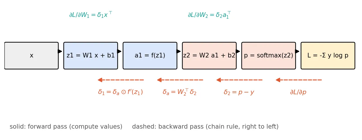
Derivation for a two-layer MLP

Take one example $(\mathbf{x}, \mathbf{y})$ with $\mathbf{x} \in \mathbb{R}^d$ and a one-hot label $\mathbf{y} \in \{0,1\}^K$. The forward pass is

$$\begin{aligned} \mathbf{z}_1 &= W_1\mathbf{x} + \mathbf{b}_1 \in \mathbb{R}^m, & \mathbf{a}_1 &= f(\mathbf{z}_1) \in \mathbb{R}^m, \\ \mathbf{z}_2 &= W_2\mathbf{a}_1 + \mathbf{b}_2 \in \mathbb{R}^K, & \mathbf{p} &= \operatorname{softmax}(\mathbf{z}_2), \qquad L = -\textstyle\sum_k y_k \log p_k , \end{aligned}$$

with $W_1 \in \mathbb{R}^{m\times d}$, $W_2 \in \mathbb{R}^{K\times m}$, and $f$ an element-wise activation. Define the error signal of a layer as the gradient of the loss with respect to its pre-activation, $\boldsymbol{\delta}_\ell = \partial L/\partial \mathbf{z}_\ell$.

Step 1, output layer. From the previous section, softmax with cross-entropy gives

$$\boldsymbol{\delta}_2 = \frac{\partial L}{\partial \mathbf{z}_2} = \mathbf{p} - \mathbf{y} \in \mathbb{R}^K .$$

Step 2, output weights. Since $z_{2,k} = \sum_j W_{2,kj}\, a_{1,j} + b_{2,k}$, we have $\partial z_{2,k}/\partial W_{2,kj} = a_{1,j}$, so

$$\frac{\partial L}{\partial W_2} = \boldsymbol{\delta}_2\, \mathbf{a}_1^\top \in \mathbb{R}^{K\times m}, \qquad \frac{\partial L}{\partial \mathbf{b}_2} = \boldsymbol{\delta}_2 .$$

The gradient of a weight is (error at its output) times (activation at its input). The shapes match $W_2$, which is a useful check.

Step 3, back through the linear layer. Each hidden activation $a_{1,j}$ affects every output, so its gradient sums over them: $\partial L/\partial a_{1,j} = \sum_k \delta_{2,k} W_{2,kj}$, or in matrix form

$$\frac{\partial L}{\partial \mathbf{a}_1} = W_2^\top \boldsymbol{\delta}_2 \in \mathbb{R}^m .$$

Step 4, back through the activation. Because $f$ acts element by element, its Jacobian is diagonal, and the chain rule becomes an element-wise product:

$$\boldsymbol{\delta}_1 = \frac{\partial L}{\partial \mathbf{z}_1} = \big(W_2^\top \boldsymbol{\delta}_2\big) \odot f'(\mathbf{z}_1) .$$

Step 5, first-layer weights. Exactly as in Step 2,

$$\frac{\partial L}{\partial W_1} = \boldsymbol{\delta}_1\, \mathbf{x}^\top \in \mathbb{R}^{m\times d}, \qquad \frac{\partial L}{\partial \mathbf{b}_1} = \boldsymbol{\delta}_1 .$$

For a deeper network, Steps 3 to 5 simply repeat: $\boldsymbol{\delta}_{\ell} = (W_{\ell+1}^\top \boldsymbol{\delta}_{\ell+1}) \odot f'(\mathbf{z}_\ell)$ and $\partial L/\partial W_\ell = \boldsymbol{\delta}_\ell\, \mathbf{a}_{\ell-1}^\top$. For a mini-batch of $N$ examples, the loss is the average, so each gradient is the average of the per-example gradients.

From scratch in NumPy, with a gradient check

The code below stores examples as rows (X has shape $N \times d$), which is the usual convention in code. Then X @ W1 with W1 of shape $d \times m$ plays the role of $W_1\mathbf{x}$ in the math, and every formula above appears transposed: for example dW2 = A1.T @ dZ2 is $\boldsymbol{\delta}_2\mathbf{a}_1^\top$ stacked over the batch. The gradient check compares one analytic derivative with a central finite difference, $\big(L(w + \epsilon) - L(w - \epsilon)\big)/2\epsilon$. If they agree to many digits, the backward pass is correct. Always do this when you write gradients by hand.

import numpy as np
from sklearn.datasets import make_moons

rng = np.random.default_rng(0)
X, y = make_moons(n_samples=200, noise=0.2, random_state=0)
N, d, h, K = X.shape[0], 2, 16, 2
Y = np.eye(K)[y]                                   # one-hot targets, (N, K)

# He-style initialization (std = sqrt(2 / fan_in))
W1 = rng.normal(0, np.sqrt(2 / d), (d, h)); b1 = np.zeros(h)
W2 = rng.normal(0, np.sqrt(2 / h), (h, K)); b2 = np.zeros(K)

def forward(X, W1, b1, W2, b2):
    Z1 = X @ W1 + b1                               # (N, h)
    A1 = np.maximum(Z1, 0)                         # ReLU
    Z2 = A1 @ W2 + b2                              # (N, K) logits
    Z2 = Z2 - Z2.max(axis=1, keepdims=True)        # numerical stability
    P = np.exp(Z2) / np.exp(Z2).sum(axis=1, keepdims=True)
    loss = -np.mean(np.sum(Y * np.log(P + 1e-12), axis=1))
    return Z1, A1, P, loss

def backward(X, Z1, A1, P, W2):
    dZ2 = (P - Y) / N                              # delta at the output
    dW2 = A1.T @ dZ2;  db2 = dZ2.sum(axis=0)
    dA1 = dZ2 @ W2.T
    dZ1 = dA1 * (Z1 > 0)                           # ReLU'(z) = 1[z > 0]
    dW1 = X.T @ dZ1;   db1 = dZ1.sum(axis=0)
    return dW1, db1, dW2, db2

# Gradient check on one entry of W1 (central difference)
Z1, A1, P, loss = forward(X, W1, b1, W2, b2)
dW1, db1, dW2, db2 = backward(X, Z1, A1, P, W2)
eps = 1e-6; E = np.zeros_like(W1); E[0, 3] = eps
num = (forward(X, W1 + E, b1, W2, b2)[3] - forward(X, W1 - E, b1, W2, b2)[3]) / (2 * eps)
print(f"analytic {dW1[0, 3]:.8f}  numeric {num:.8f}")

# Plain gradient descent
lr = 0.5
for step in range(2000):
    Z1, A1, P, loss = forward(X, W1, b1, W2, b2)
    dW1, db1, dW2, db2 = backward(X, Z1, A1, P, W2)
    W1 -= lr * dW1; b1 -= lr * db1; W2 -= lr * dW2; b2 -= lr * db2
acc = (P.argmax(axis=1) == y).mean()
print(f"final loss {loss:.3f}, train accuracy {acc:.3f}")
# analytic -0.01941581  numeric -0.01941581
# final loss 0.063, train accuracy 0.970

In practice you never write the backward pass yourself: frameworks such as PyTorch record the forward computation and run this exact procedure automatically when you call loss.backward(). Writing it once by hand is still the best way to understand what that call does, and why it fails when something in the graph has a zero derivative.

Training II: making optimization work

Plain version. Knowing the gradient is not enough. You also need a sensible starting point (initialization), a rule for turning gradients into steps (the optimizer), a step size that changes over time (the schedule), a choice of how many examples to look at per step (the batch size), and a guard against occasional huge steps (clipping).

Vanishing and exploding gradients

Unroll the recursion $\boldsymbol{\delta}_\ell = (W_{\ell+1}^\top \boldsymbol{\delta}_{\ell+1}) \odot f'(\mathbf{z}_\ell)$ across $L$ layers and the gradient at the first layer contains a product of $L$ weight matrices and $L$ activation derivatives. If the typical factor is below 1, the product shrinks exponentially with depth and the early layers barely learn: vanishing gradients. With the sigmoid, every $f'$ is at most $0.25$, so ten layers can shrink the signal by a factor of up to $0.25^{10} \approx 10^{-6}$. If the typical factor is above 1, for example because the initial weights are too large, the product grows exponentially, updates become huge, and the loss turns into inf or NaN: exploding gradients.

The remedies, each covered below, attack the product from different sides:

• activations whose derivative is 1 over a wide range (ReLU and its smooth relatives);
• initialization that keeps signal size constant from layer to layer;
• normalization layers that re-standardize activations;
• residual connections, which give the gradient a path with factor 1 (the last main section);
• gradient clipping, the standard emergency brake for explosions.

Other practices sometimes listed, such as fine-tuning a pre-trained model or using a smaller network, make training easier overall, but they do not directly fix the gradient problem.

Weight initialization

If all weights start equal, every hidden unit computes the same thing and receives the same gradient, and they stay identical forever. So weights start random. The scale matters: we want the variance of activations (forward) and of gradients (backward) to stay roughly constant from layer to layer. For a linear layer with $n_{\text{in}}$ inputs and $n_{\text{out}}$ outputs:

• Xavier (Glorot) initialization [17] balances the forward and backward conditions for symmetric activations such as tanh: $\operatorname{Var}(W_{ij}) = \dfrac{2}{n_{\text{in}} + n_{\text{out}}}$, for example uniform on $\big[-\sqrt{6/(n_{\text{in}} + n_{\text{out}})},\ \sqrt{6/(n_{\text{in}} + n_{\text{out}})}\big]$.
• He (Kaiming) initialization [18] accounts for ReLU zeroing about half its inputs, which halves the variance at every layer, by doubling the scale: $\operatorname{Var}(W_{ij}) = \dfrac{2}{n_{\text{in}}}$, for example $W_{ij} \sim \mathcal{N}(0, 2/n_{\text{in}})$.

Biases usually start at zero. He et al. showed that this initialization lets very deep ReLU networks be trained from scratch [18]. The NumPy example above uses it.

Optimizers

Every optimizer below is a variant of stochastic gradient descent (SGD): estimate the gradient on a small random mini-batch, take a step against it, repeat. Write $\mathbf{g}_t = \nabla_\theta L_{\text{batch}}(\theta_t)$ for the mini-batch gradient at step $t$, $\theta$ for all parameters and $\eta$ for the learning rate.

SGD. $\theta_{t+1} = \theta_t - \eta\,\mathbf{g}_t$. Simple and memory-free, but it zigzags in narrow valleys and moves slowly along flat directions.

SGD with momentum. Keep a running velocity: $\mathbf{v}_{t+1} = \mu\,\mathbf{v}_t + \mathbf{g}_t$, $\theta_{t+1} = \theta_t - \eta\,\mathbf{v}_{t+1}$, with $\mu$ around 0.9. Like a heavy ball rolling downhill, it averages out the zigzag and builds speed along consistent directions.

Adam (Kingma and Ba [19]) keeps two running averages per parameter, of the gradient and of its square:

$$\begin{aligned} \mathbf{m}_t &= \beta_1 \mathbf{m}_{t-1} + (1 - \beta_1)\,\mathbf{g}_t, & \mathbf{v}_t &= \beta_2 \mathbf{v}_{t-1} + (1 - \beta_2)\,\mathbf{g}_t^{2}, \\ \hat{\mathbf{m}}_t &= \frac{\mathbf{m}_t}{1 - \beta_1^t}, & \hat{\mathbf{v}}_t &= \frac{\mathbf{v}_t}{1 - \beta_2^t}, \qquad \theta_t = \theta_{t-1} - \eta\,\frac{\hat{\mathbf{m}}_t}{\sqrt{\hat{\mathbf{v}}_t} + \epsilon}, \end{aligned}$$

where squares, square roots and division are element-wise, $\beta_1 \approx 0.9$ and $\beta_2 \approx 0.999$ are decay rates, and $\epsilon$ is a small constant. The first average is momentum. Dividing by the root of the second gives every parameter its own step size, which is the idea of RMSprop that Adam builds on [19]: parameters with consistently large gradients take smaller steps, rarely updated ones take larger steps. The bias correction $1/(1-\beta^t)$ fixes the fact that both averages start at zero and would otherwise be too small in the first steps.

AdamW (Loshchilov and Hutter [20]). Weight decay shrinks weights toward zero at every step. For plain SGD this is the same as adding an L2 penalty $\tfrac{\lambda}{2}\lVert\theta\rVert^2$ to the loss. For Adam it is not: an L2 term enters $\mathbf{g}_t$ and is then divided by $\sqrt{\hat{\mathbf{v}}_t}$, so weights with large gradients are regularized less. AdamW decouples the decay from the adaptive step:

$$\theta_t = \theta_{t-1} - \eta\left(\frac{\hat{\mathbf{m}}_t}{\sqrt{\hat{\mathbf{v}}_t} + \epsilon} + \lambda\,\theta_{t-1}\right).$$

The authors showed this improves Adam’s generalization [20], and AdamW is now the most common optimizer for Transformers and large language models. In PyTorch, torch.optim.Adam(..., weight_decay=λ) is the coupled L2 version and torch.optim.AdamW is the decoupled one.

Newer optimizers (brief notes). Two recent alternatives are worth knowing by name. Lion was found by an automated program search [21]: it keeps only a momentum buffer (so it uses less memory than Adam) and updates every parameter by the sign of an interpolated momentum, so all updates have the same magnitude; it needs a smaller learning rate than AdamW. Muon [22] applies to the 2-D weight matrices of hidden layers: it takes the momentum update and approximately orthogonalizes it with a few Newton–Schulz iterations, while embeddings, output layers, biases and other scalar or vector parameters are still trained with AdamW. Liu et al. report that, with weight decay and per-parameter update scaling added, Muon reached about twice the compute efficiency of AdamW in their compute-optimal large-language-model training experiments [23]. These are active research topics; AdamW remains the safe default.

Learning-rate schedules

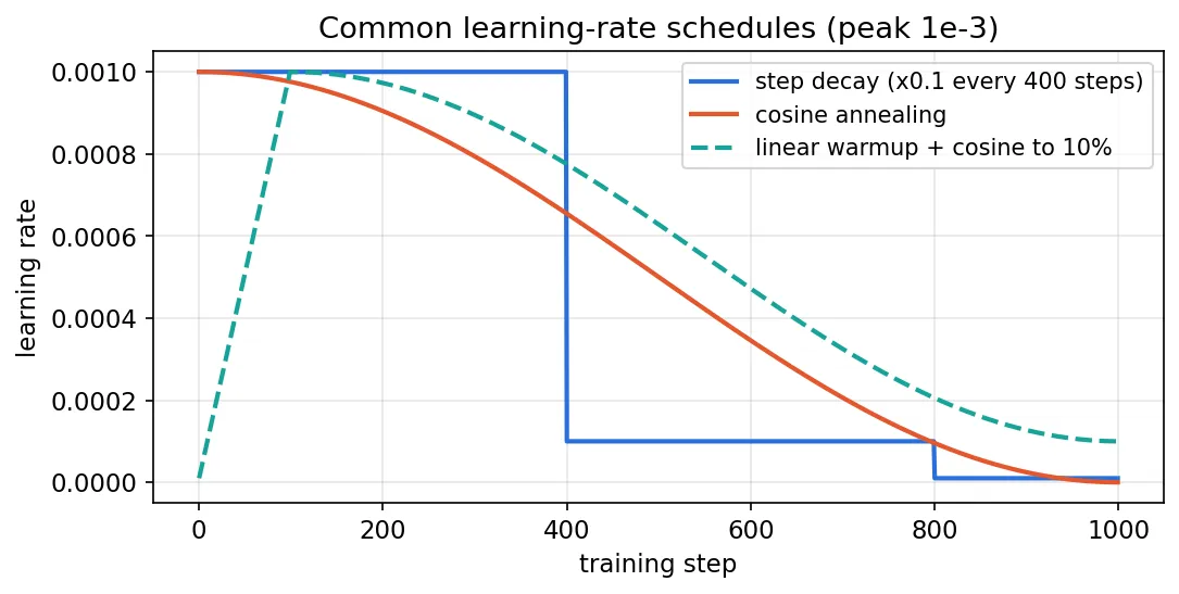
The learning rate is usually the most important hyperparameter. A rate that is fine early in training is often too large later, when the model needs small, careful steps, so the rate is varied over time (Figure 6).

• Step decay: multiply the rate by a factor such as 0.1 at fixed epochs. Traditional for CNN training with SGD.
• Cosine annealing: $\eta_t = \eta_{\min} + \tfrac12(\eta_{\max} - \eta_{\min})\big(1 + \cos(\pi t / T)\big)$, a smooth decay from $\eta_{\max}$ to $\eta_{\min}$ over $T$ steps; SGDR [24] combined it with periodic warm restarts.
• Warmup: increase the rate linearly from near zero over the first few hundred or thousand steps. Early in training, Adam’s second-moment estimates are noisy and the weights are far from any good region, and a full-size step can be destabilizing.

As a concrete recipe from a published large model, LLaMA was trained with AdamW ($\beta_1 = 0.9$, $\beta_2 = 0.95$), weight decay 0.1, gradient clipping at 1.0, 2,000 warmup steps, and a cosine schedule ending at 10% of the peak rate [12].

Mini-batches, iterations and epochs

A mini-batch (often just “batch”) is the small random subset of $B$ examples used for one gradient estimate. One iteration is one parameter update, using one mini-batch. One epoch is one full pass over the training set, which takes $\lceil N/B \rceil$ iterations for $N$ examples. For example, $N = 50{,}000$ and $B = 128$ give 391 iterations per epoch.

The batch size $B$ affects both speed and the result, and bigger is not always better:

• Small batches give noisy gradient estimates (the variance of the mini-batch mean falls roughly like $1/B$), so the loss curve is jumpy and each epoch takes many steps with poor hardware utilization.
• Large batches give stable gradients and run efficiently in parallel on GPUs, but each epoch has fewer updates, and they tend to generalize worse when other settings are kept fixed. Keskar et al. found that large-batch training tends to converge to sharp minima, where the loss rises steeply around the solution, while small-batch training, thanks to its gradient noise, tends to find flat minima, which generalize better [25].

In practice, choose the largest batch that fits comfortably in memory and still trains well, and retune the learning rate when you change $B$; the two interact strongly.

Gradient clipping

Even in a well-designed network, a rare batch can produce a huge gradient. Gradient-norm clipping rescales the whole gradient when its norm exceeds a threshold $c$:

$$\mathbf{g} \leftarrow \mathbf{g}\cdot\min\!\left(1, \frac{c}{\lVert \mathbf{g} \rVert}\right),$$

where $\lVert\mathbf{g}\rVert$ is the norm of all parameter gradients concatenated. It keeps the direction but limits the step size, which is the standard defense against exploding gradients, especially in recurrent networks and Transformers [3]. A threshold of 1.0 is a common choice.

Putting it together in PyTorch

The snippet trains a small MLP on make_moons with mini-batches, AdamW, a cosine schedule and gradient clipping. It runs on a CPU in seconds.

import torch, torch.nn as nn
from sklearn.datasets import make_moons
from sklearn.model_selection import train_test_split

torch.manual_seed(0)
X, y = make_moons(n_samples=1000, noise=0.25, random_state=0)
Xtr, Xva, ytr, yva = train_test_split(X, y, test_size=0.3, random_state=0)
Xtr, Xva = torch.tensor(Xtr, dtype=torch.float32), torch.tensor(Xva, dtype=torch.float32)
ytr, yva = torch.tensor(ytr), torch.tensor(yva)

model = nn.Sequential(
    nn.Linear(2, 64), nn.ReLU(),
    nn.Linear(64, 64), nn.ReLU(),
    nn.Linear(64, 2),               # logits: no softmax here
)
loss_fn = nn.CrossEntropyLoss()     # applies log-softmax internally
opt = torch.optim.AdamW(model.parameters(), lr=1e-2, weight_decay=1e-2)
sched = torch.optim.lr_scheduler.CosineAnnealingLR(opt, T_max=200)

for epoch in range(200):
    model.train()
    perm = torch.randperm(len(Xtr))
    for i in range(0, len(Xtr), 64):                # mini-batches of 64
        idx = perm[i:i + 64]
        loss = loss_fn(model(Xtr[idx]), ytr[idx])
        opt.zero_grad()
        loss.backward()                              # backpropagation
        torch.nn.utils.clip_grad_norm_(model.parameters(), max_norm=1.0)
        opt.step()
    sched.step()

model.eval()
with torch.no_grad():
    acc = (model(Xva).argmax(dim=1) == yva).float().mean().item()
print(f"validation accuracy: {acc:.3f}")   # about 0.94

Note model.train() and model.eval(): they switch layers such as dropout and BatchNorm between their training and inference behavior. Forgetting eval() at test time is a classic bug.

Generalization: underfitting, overfitting and regularization

Plain version. The goal is not to do well on the training data; it is to do well on data the model has never seen. A model can fail in two opposite ways: it can be too weak to learn even the training data (underfitting), or it can memorize the training data, noise included, and fail on new data (overfitting).

Capacity and the two failure modes

A model’s capacity is, informally, how complex a function it can fit; it grows with the number of parameters, depth and width, and training time. As capacity increases, training error keeps falling, while validation error first falls and then rises again once the model starts fitting noise. The gap between the two is the generalization gap [3].

• Underfitting: the training error itself is high. The model, or the training procedure, cannot capture the pattern.
• Overfitting: the training error is low but the validation or test error is much higher.

What to do about underfitting, in order:

1. Check the code and data first. A bug, mismatched inputs and labels, wrong preprocessing, or a loss applied to the wrong tensor all look like underfitting.
2. Increase capacity: a wider or deeper model, or a better architecture.
3. Improve optimization: train longer, tune the learning rate and schedule, switch optimizer, check initialization and normalization.

Making the model smaller never fixes underfitting; it lowers capacity further. A smaller model can be a reasonable choice for speed or memory once accuracy is adequate, but that is an efficiency decision, not a cure.

What to do about overfitting: use more or more varied data, add regularization (below), reduce capacity, and stop early. It is also worth checking that the training and validation sets really come from the same distribution; a mismatch between them looks like overfitting but needs a data fix, not a regularizer.

Reading a loss curve

Plot both the training and the validation loss against iterations or epochs. Four patterns cover most situations:

• A. Both curves flat from the start. If the loss is high, the model is not learning at all: suspect a bug, a far too small or large learning rate, or a model/data mismatch. If the loss is already low, the task may be very easy, or each logged point covers so many iterations that the curve’s shape is hidden; log more often.
• B. Training loss keeps falling, validation loss turns upward. Classic overfitting. Keep the parameters from the point of lowest validation loss (early stopping) and add regularization.
• C. Both curves fall and level off close together. Either the model is near its best, which is common when training and validation data are very similar, or both are still high, which is underfitting: train longer or increase capacity.
• D. Validation loss above training loss, but both still decreasing steadily. The normal, healthy situation. Keep training and keep the checkpoint with the lowest validation loss.

Regularization tools

Figure 7 shows overfitting and two cures on purpose. A wide MLP (two hidden layers of 256 units) is trained on only 100 noisy two-moons points. Without regularization the training loss falls toward zero while the validation loss reaches its minimum early and then climbs steeply. Weight decay and dropout both slow the climb dramatically.

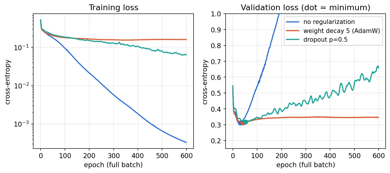
Weight decay (L2 regularization). Penalize large weights by adding $\tfrac{\lambda}{2}\lVert\theta\rVert^2$ to the loss, or, with Adam, use decoupled decay (AdamW). Large weights let a network make sharp, wiggly boundaries around individual points; keeping them small favors smoother functions. In Figure 7, decoupled decay with $\lambda = 5$ keeps the validation loss almost flat after its minimum.

Dropout (Srivastava et al. [27]). During training, set each hidden unit to zero with probability $p$, independently for every example and step, and scale the survivors by $1/(1-p)$ so the expected activation is unchanged (“inverted dropout”). At test time, use all units with no scaling. Each step thus trains a different thinned sub-network; units cannot rely on specific partners and must learn features that are useful on their own, and the full network at test time behaves like an average of many thinned networks [27]. This is why model.eval() matters.

Data augmentation. Create new training examples by applying transformations that do not change the label: flips, crops, small rotations, color jitter and noise for images. It is often the single most effective regularizer in vision, because it teaches the invariances directly. It must respect the task: a horizontal flip is fine for cats, not for reading text.

Early stopping. Monitor the validation loss during training and keep the parameters from the epoch where it was lowest; stop when it has not improved for a set number of epochs (the “patience”). It costs nothing, needs no change to the model, and acts as a regularizer by limiting how far the parameters can travel from their initialization [3].

More data and better strategy. The other levers the original notes list are worth repeating: more training data is the most reliable cure for overfitting; a stronger architecture (deeper, or better structured, so that it converges well) helps when the model underfits; and a better training strategy (optimizer, learning-rate schedule, batch size) helps both.

Residual connections and the road to Transformers

Plain version. If you stack many layers, each must pass the signal on intact as well as improve it, which turns out to be hard. A residual connection gives every block an express lane: the block only has to learn a correction that is added to its input.

He et al. observed that adding more plain layers to an already deep network made even the training error worse, which is an optimization problem rather than overfitting [28]. Their residual block computes

$$\mathbf{y} = \mathbf{x} + F(\mathbf{x}),$$

where $\mathbf{x}$ is the block’s input and $F$ is a small stack of layers (in ResNet, convolutions with BatchNorm and ReLU). If the best thing a block can do is nothing, it only has to push $F$ toward zero, which is easy. The backward pass shows why it trains well:

$$\frac{\partial \mathbf{y}}{\partial \mathbf{x}} = I + \frac{\partial F}{\partial \mathbf{x}},$$

where $I$ is the identity matrix. The identity term passes the gradient straight through every block, so the product over many blocks no longer has to shrink to zero. With residual connections, He et al. trained networks with up to 152 layers on ImageNet and won several ILSVRC 2015 tasks [28].

The Transformer (Vaswani et al. [29]) combines every idea in this tutorial. Each block has two sub-layers, multi-head self-attention (which uses softmax to mix information between positions) and a position-wise MLP, and each sub-layer is wrapped in a residual connection with LayerNorm. The original paper normalized after the addition; many recent models, LLaMA among them, normalize the sub-layer input instead (pre-normalization) and use RMSNorm and SwiGLU [12]:

$$\mathbf{h} = \mathbf{x} + \operatorname{Attention}\big(\operatorname{Norm}(\mathbf{x})\big), \qquad \mathbf{y} = \mathbf{h} + \operatorname{FFN}\big(\operatorname{Norm}(\mathbf{h})\big).$$

Since 2017 this design has spread from machine translation to language modeling, vision, speech and more, and it is the basis of today’s large language models. The trained recipe is the one from this tutorial too: AdamW, warmup and cosine decay, gradient clipping, and weight decay [12]. The deep-learning track picks up from here with convolutional networks and Transformers for images, starting with image classification.

Modern view

The basic toolkit above has been stable for several years; research continues on why it works and on better versions of each piece. The following reviews are good guides, each from a different angle.

The big picture: LeCun, Bengio and Hinton [2] (Nature, 2015). This short review is still the clearest statement of what deep learning is: representation learning with many layers, where each layer transforms the previous representation into a more abstract one and the features are learned from data with backpropagation rather than engineered. It walks through supervised learning with SGD, the role of ReLU, convolutional networks for images, recurrent networks for sequences, and distributed representations, and it closes by predicting that unsupervised learning and the combination of representation learning with reasoning would matter more in the future. For a textbook treatment of every topic in this tutorial, including the maximum-likelihood view of loss functions, regularization and optimization, the book by Goodfellow, Bengio and Courville [3] remains the standard reference.

Optimization: Sun [26]. Sun’s survey asks “when and why can a neural network be successfully trained?” and organizes the answer in three parts: problems with the gradient (explosion, vanishing) and their fixes through careful initialization and normalization; the practical algorithms (SGD, adaptive methods such as Adam, and distributed training) with their convergence theory; and the global picture of the loss landscape, including bad local minima, mode connectivity, the lottery-ticket hypothesis and the infinite-width limit. It is a good bridge from the practice above to theory.

Normalization: Huang et al. [16] (IEEE TPAMI, 2023). This survey gives a unified view of normalization methods from the perspective of optimization, and a taxonomy that splits any method into its normalization area, normalization operation and representation recovery. It covers the history from BatchNorm on, the analyses of why normalization speeds training and helps generalization, and applications in different domains. Read it to see BatchNorm, LayerNorm, group-wise and weight-based normalization as points in one design space.

Activation functions: Dubey, Singh and Chaudhuri [7] (Neurocomputing, 2022). This survey classifies activation functions into logistic sigmoid/tanh-based, ReLU-based, ELU-based and learning-based families, characterizes them by properties such as output range, monotonicity and smoothness, and benchmarks 18 of them across network types and data. Its practical message is that no single activation is best everywhere; the choice interacts with the architecture and the data.

Where things stand (2023–2026). Several convergences are visible in published model recipes:

• Architecture. The pre-normalized Transformer block with residual connections is the dominant architecture for language and increasingly for vision; RMSNorm and SwiGLU, as in LLaMA [12], are common defaults in large language models.
• Optimization. AdamW [20] with linear warmup, a cosine (or similar) decay, and gradient clipping is the standard recipe. Optimizers that look beyond per-coordinate scaling are an active area: Lion [21] uses sign updates and less memory, and Muon [22] orthogonalizes matrix updates, with reported compute-efficiency gains at scale [23]. How robust such gains are across tasks and scales is still being studied, which is why AdamW remains the safe choice.
• Generalization. The sharp-versus-flat-minima view [25] is a useful intuition rather than a complete theory, and why heavily over-parameterized networks generalize as well as they do is still an open question; Sun’s survey [26] summarizes the main lines of attack.

Open problems. A reliable theory of generalization for deep networks; principled rules for choosing the learning rate, batch size and schedule together, especially when scaling models up; understanding exactly how normalization, residual connections and adaptive optimizers interact; and making training stable at very large scale without the many small tricks that current recipes rely on.

Key takeaways

• A perceptron is a linear score followed by a step function and trained by a mistake-driven rule; logistic regression uses a sigmoid probability and cross-entropy. Similar structure, different methods, and only the smooth one can be stacked and trained by gradients.
• Hidden layers with nonlinear activations are what make networks more than linear models. One wide hidden layer can in principle approximate any continuous function, but that is an existence result; depth makes useful functions easier to represent and learn. There is no fixed layer count that defines “deep”.
• ReLU-family activations (ReLU, Leaky ReLU, GELU, SiLU) keep gradients alive; sigmoid and softmax belong mostly at the output; SwiGLU is the modern feed-forward choice in Transformers. BatchNorm normalizes over the batch, LayerNorm and RMSNorm over the features of each sample.
• Match the head to the task: linear plus MSE for regression, sigmoid plus binary cross-entropy for binary or multi-label, softmax plus cross-entropy for multi-class. In each case the output gradient is prediction minus target.
• Backpropagation is the chain rule applied from the loss backward: $\boldsymbol{\delta}_\ell = (W_{\ell+1}^\top\boldsymbol{\delta}_{\ell+1})\odot f'(\mathbf{z}_\ell)$ and $\partial L/\partial W_\ell = \boldsymbol{\delta}_\ell\mathbf{a}_{\ell-1}^\top$. Check hand-written gradients numerically.
• Practical training: He or Xavier initialization, AdamW with warmup and a decaying schedule, gradient clipping, and a batch size chosen with the learning rate, not “as large as possible”.
• Underfitting means high training error and calls for more capacity or better optimization, never a smaller model; overfitting calls for more data, augmentation, weight decay, dropout and early stopping.
• Residual connections make very deep networks trainable, and the Transformer is these ideas combined.

Exercises

1. Perceptron by hand. Run the perceptron rule on the AND data with $\eta = 1$, $\mathbf{w} = \mathbf{0}$, $b = 0$, visiting the points in the order $(0,0), (0,1), (1,0), (1,1)$. Write down $\mathbf{w}$ and $b$ after each update until an epoch passes with no mistakes. Then explain in one sentence why the same procedure on XOR never stops.

Hint

With the strict test $z > 0$, the first point $(0,0)$ has $z = 0$, so it is predicted 0 and is correct. The first mistake is $(1,1)$, which gives $\mathbf{w} = (1,1)$, $b = 1$. Keep going: each mistake on a 0-labeled point subtracts $\mathbf{x}$ and 1, each mistake on the 1-labeled point adds them. With this order there are ten updates over five epochs, and the sixth epoch is error-free with $\mathbf{w} = (2, 1)$, $b = -2$, that is, the line $2x_1 + x_2 = 2$. A different visiting order gives a different, equally valid line. For XOR, no $(\mathbf{w}, b)$ classifies all four points correctly, so some point is always wrong and an update always happens.

2. How fast do sigmoid gradients vanish? Show that $\sigma'(x) = \sigma(x)(1 - \sigma(x)) \le 1/4$. Then consider a chain of 20 sigmoid layers with all weights equal to 1. What is the largest factor by which the gradient can be multiplied on its way back? Repeat the reasoning for ReLU with active units.

Hint

$s(1-s)$ with $s \in (0,1)$ is a downward parabola with maximum $1/4$ at $s = 1/2$. Twenty factors of at most $1/4$ give at most $4^{-20} \approx 9 \times 10^{-13}$. For an active ReLU unit, $f' = 1$, so the activations contribute no shrinkage at all; only the weights do, which is why initialization matters.

3. The prediction-minus-target gradient. Using $\partial p_k/\partial z_j = p_k(\delta_{kj} - p_j)$, prove that for $L = -\sum_k y_k \log p_k$ with a one-hot $\mathbf{y}$, $\partial L/\partial z_j = p_j - y_j$. Then show the same result for the sigmoid with binary cross-entropy.

Hint

$\partial L/\partial z_j = -\sum_k (y_k/p_k)\, p_k(\delta_{kj} - p_j) = -\sum_k y_k \delta_{kj} + p_j \sum_k y_k = -y_j + p_j$, since $\sum_k y_k = 1$. For the sigmoid, $\partial \ell/\partial \hat{p} = -y/\hat{p} + (1-y)/(1-\hat{p})$ and $\partial \hat{p}/\partial z = \hat{p}(1-\hat{p})$; multiply and simplify to $\hat{p} - y$.

4. Extend the gradient check. In the NumPy example, check every entry of W2, b1 and b2 (not just one entry of W1) against finite differences, and report the maximum relative error $\lvert a - n\rvert / \max(\lvert a\rvert, \lvert n\rvert, 10^{-12})$. Then deliberately introduce a bug, for example drop the * (Z1 > 0) factor, and see how large the error becomes.

Hint

Loop over np.ndindex(param.shape), perturb one entry by $\pm 10^{-6}$, and recompute the loss. A correct implementation gives relative errors around $10^{-7}$ or smaller (a few entries next to ReLU kinks can be larger). Removing the ReLU derivative makes errors of order 1 appear in W1 and b1, while W2 and b2 stay correct, because the bug is only in the backward path below the hidden layer.

5. Iterations, epochs and batch size. A dataset has 60,000 training images. (a) How many iterations make one epoch with $B = 32$, and with $B = 1{,}024$? (b) If you train both for 20 epochs, how many parameter updates does each make? (c) Based on the batch-size discussion, give two reasons the $B = 1{,}024$ run might reach a worse validation accuracy with the same learning rate, and one change that could help.

Hint

(a) $\lceil 60000/32 \rceil = 1875$ and $\lceil 60000/1024 \rceil = 59$. (b) 37,500 versus 1,180 updates. (c) Far fewer updates in the same number of epochs, and less gradient noise, which the sharp-minima findings associate with worse generalization. Tuning the learning rate for the new batch size (typically larger, with warmup) and training for more epochs are the usual adjustments.

6. Diagnose the curve. A colleague’s network has a training loss that drops quickly at first and then stays flat at a high value; the validation loss tracks it closely. They propose halving the number of hidden units “to make it converge faster”. What is happening, what would you check first, and what would you suggest instead?

Hint

Both losses are high and close together: this is underfitting (pattern C with high values), not overfitting. First check for bugs: labels aligned with inputs, the loss applied to logits, data normalized, the learning rate sensible. Then increase capacity or improve optimization (wider or deeper model, a learning-rate schedule, longer training). Shrinking the model lowers capacity and will make underfitting worse.

References

1. Shyandram, “機器學習及類神經網路筆記 (Notes on machine learning and neural networks),” blog post (in Traditional Chinese), 2024; updated 2026. link
2. Y. LeCun, Y. Bengio and G. Hinton, “Deep learning,” Nature, vol. 521, no. 7553, pp. 436–444, 2015. doi
3. I. Goodfellow, Y. Bengio and A. Courville, Deep Learning, MIT Press, 2016. online book
4. F. Rosenblatt, “The perceptron: A probabilistic model for information storage and organization in the brain,” Psychological Review, vol. 65, pp. 386–408, 1958. doi
5. G. Cybenko, “Approximation by superpositions of a sigmoidal function,” Mathematics of Control, Signals and Systems, vol. 2, pp. 303–314, 1989. doi
6. D. E. Rumelhart, G. E. Hinton and R. J. Williams, “Learning representations by back-propagating errors,” Nature, vol. 323, pp. 533–536, 1986. doi
7. S. R. Dubey, S. K. Singh and B. B. Chaudhuri, “Activation functions in deep learning: A comprehensive survey and benchmark,” Neurocomputing, vol. 503, pp. 92–108, 2022. arXiv
8. D. Hendrycks and K. Gimpel, “Gaussian error linear units (GELUs),” arXiv:1606.08415, 2016. arXiv
9. S. Elfwing, E. Uchibe and K. Doya, “Sigmoid-weighted linear units for neural network function approximation in reinforcement learning,” Neural Networks, vol. 107, pp. 3–11, 2018. arXiv
10. P. Ramachandran, B. Zoph and Q. V. Le, “Searching for activation functions,” arXiv:1710.05941, 2017. arXiv
11. N. Shazeer, “GLU variants improve Transformer,” arXiv:2002.05202, 2020. arXiv
12. H. Touvron, T. Lavril, G. Izacard et al., “LLaMA: Open and efficient foundation language models,” arXiv:2302.13971, 2023. arXiv
13. S. Ioffe and C. Szegedy, “Batch normalization: Accelerating deep network training by reducing internal covariate shift,” in Proc. International Conference on Machine Learning (ICML), PMLR 37, pp. 448–456, 2015. PMLR
14. J. L. Ba, J. R. Kiros and G. E. Hinton, “Layer normalization,” arXiv:1607.06450, 2016. arXiv
15. B. Zhang and R. Sennrich, “Root mean square layer normalization,” in Advances in Neural Information Processing Systems (NeurIPS), 2019. arXiv
16. L. Huang, J. Qin, Y. Zhou, F. Zhu, L. Liu and L. Shao, “Normalization techniques in training DNNs: Methodology, analysis and application,” IEEE Transactions on Pattern Analysis and Machine Intelligence, vol. 45, no. 8, pp. 10173–10196, 2023. arXiv
17. X. Glorot and Y. Bengio, “Understanding the difficulty of training deep feedforward neural networks,” in Proc. International Conference on Artificial Intelligence and Statistics (AISTATS), PMLR 9, pp. 249–256, 2010. PMLR
18. K. He, X. Zhang, S. Ren and J. Sun, “Delving deep into rectifiers: Surpassing human-level performance on ImageNet classification,” in Proc. IEEE International Conference on Computer Vision (ICCV), pp. 1026–1034, 2015. arXiv
19. D. P. Kingma and J. Ba, “Adam: A method for stochastic optimization,” in Proc. International Conference on Learning Representations (ICLR), 2015. arXiv
20. I. Loshchilov and F. Hutter, “Decoupled weight decay regularization,” in Proc. International Conference on Learning Representations (ICLR), 2019. arXiv
21. X. Chen, C. Liang, D. Huang, E. Real, K. Wang, H. Pham, X. Dong, T. Luong, C.-J. Hsieh, Y. Lu and Q. V. Le, “Symbolic discovery of optimization algorithms,” in Advances in Neural Information Processing Systems (NeurIPS), 2023. arXiv
22. K. Jordan, “Muon: An optimizer for hidden layers in neural networks,” blog post, December 2024. link
23. J. Liu, J. Su, X. Yao et al., “Muon is scalable for LLM training,” arXiv:2502.16982, 2025. arXiv
24. I. Loshchilov and F. Hutter, “SGDR: Stochastic gradient descent with warm restarts,” in Proc. International Conference on Learning Representations (ICLR), 2017. arXiv
25. N. S. Keskar, D. Mudigere, J. Nocedal, M. Smelyanskiy and P. T. P. Tang, “On large-batch training for deep learning: Generalization gap and sharp minima,” in Proc. International Conference on Learning Representations (ICLR), 2017. arXiv
26. R. Sun, “Optimization for deep learning: Theory and algorithms,” arXiv:1912.08957, 2019. arXiv
27. N. Srivastava, G. Hinton, A. Krizhevsky, I. Sutskever and R. Salakhutdinov, “Dropout: A simple way to prevent neural networks from overfitting,” Journal of Machine Learning Research, vol. 15, pp. 1929–1958, 2014. JMLR
28. K. He, X. Zhang, S. Ren and J. Sun, “Deep residual learning for image recognition,” in Proc. IEEE Conference on Computer Vision and Pattern Recognition (CVPR), pp. 770–778, 2016. arXiv
29. A. Vaswani, N. Shazeer, N. Parmar, J. Uszkoreit, L. Jones, A. N. Gomez, Ł. Kaiser and I. Polosukhin, “Attention is all you need,” in Advances in Neural Information Processing Systems (NeurIPS), 2017. arXiv