ML 01 · Introduction to Machine Learning

What you’ll learn

• What “learning from data” means, and how it differs from writing rules by hand, using small images of handwritten digits as the running example.
• The main learning paradigms: supervised (regression and classification), unsupervised (clustering, dimensionality reduction, anomaly detection), self-supervised, and reinforcement learning, including how reinforcement learning from human feedback (RLHF) tunes chat models.
• The vocabulary of a learning problem: model $f_{w,b}(x)$, parameters, features, targets, predictions, training/validation/test sets and cost functions.
• Linear regression with the mean squared error cost, and gradient descent to minimize it: the update rule, the learning rate, convergence, and batch versus mini-batch versus stochastic updates.
• Why feature scaling matters, how logistic regression turns a line into a classifier with the sigmoid and cross-entropy loss, and how to detect and fix overfitting with validation data and L2 regularization.
• How to report results honestly with accuracy, precision, recall and MSE.

The big picture

Most programs are recipes: a person thinks hard about a problem and writes down every step. Machine learning flips this. We write a flexible program with many adjustable numbers, show it many examples of the job done correctly, and let an algorithm adjust the numbers until the program does the job well. The examples replace the recipe.

Why this matters: almost every modern computer-vision system, from phone face unlock to medical image analysis, is a learned model, not a hand-written program. The ideas in this tutorial (a model with parameters, a cost that measures error, gradient descent that lowers the cost, and separate data to check the result) are the same ideas that train today’s largest neural networks. Only the size of the model changes. Once these few ideas are clear, the rest of the series (ML 02 and the deep-learning tutorials) is mostly about which model and which cost.

What is machine learning?

Plain version. A machine-learning system improves at a task by looking at data, instead of having every decision written by a programmer.

Learning instead of programming

The idea is old. In 1959, Arthur Samuel described a program that learned to play checkers better than he did, by playing many games and adjusting how it scored board positions [2]. His point was that a computer which learns from experience removes much of the detailed, hand-written programming the task would otherwise need. The famous one-line definition, machine learning as the “field of study that gives computers the ability to learn without being explicitly programmed”, is a later paraphrase of this idea, usually attributed to Samuel, rather than a sentence from his paper.

A more operational definition, common in textbooks, has three parts: a task (for example, recognizing digits), a performance measure (the fraction recognized correctly), and experience (a collection of labeled digit images). A program learns if its performance on the task improves with experience [3], [7].

An image example: rules versus learning

Our running example is the scikit-learn digits dataset [5], [6]: 1,797 grayscale images of handwritten digits, each only $8 \times 8$ pixels with values from 0 to 16. As in Images as Arrays, each image is just a small array of numbers, and flattening it gives a vector of 64 numbers.

Suppose we only need to tell a 0 from a 1. A programmer might write a rule: “a 1 is thin, a 0 is wide, so count how many columns contain ink; five columns or fewer means 1.” This rule is easy to read, and it is right for most upright 1s. But people write 1s with slants, serifs and bases, and a slanted 1 covers as many columns as a 0 (Figure 1). The rule gets about 79% of the cases right. Fixing it means more rules (“unless it slants…”), and each new rule creates new exceptions.

The machine-learning approach writes no digit-specific rule. It picks a flexible family of functions (here, logistic regression, which we build later), and lets an algorithm choose the 65 numbers inside it from examples. On held-out images, it separates 0s from 1s perfectly, and exactly the same code handles all ten digits with no new rules:

import numpy as np
from sklearn.datasets import load_digits
from sklearn.model_selection import train_test_split
from sklearn.linear_model import LogisticRegression

digits = load_digits()                       # 1,797 images, 8x8 pixels, values 0..16
X, y = digits.data, digits.target            # X: (1797, 64) flattened pixels; y: 0..9

# Hand-written rule for "0 versus 1": a 1 is thin, a 0 is wide.
keep = (y == 0) | (y == 1)
imgs, labels = digits.images[keep], y[keep]
width = (imgs.max(axis=1) > 4).sum(axis=1)   # how many columns contain ink
rule = np.where(width <= 5, 1, 0)
print("hand rule, 0 vs 1:", round((rule == labels).mean(), 3))           # 0.789

# Learned rule for the same task, judged on images it never saw.
X01 = imgs.reshape(len(imgs), -1)
Xa, Xb, ya, yb = train_test_split(X01, labels, test_size=0.3, random_state=0)
print("learned, 0 vs 1:", LogisticRegression(max_iter=1000).fit(Xa, ya).score(Xb, yb))   # 1.0

# The same recipe scales to all ten digits with no new rules.
X_tr, X_te, y_tr, y_te = train_test_split(X, y, test_size=0.25, random_state=0)
print("learned, 10 digits:",
      round(LogisticRegression(max_iter=5000).fit(X_tr, y_tr).score(X_te, y_te), 3))  # 0.953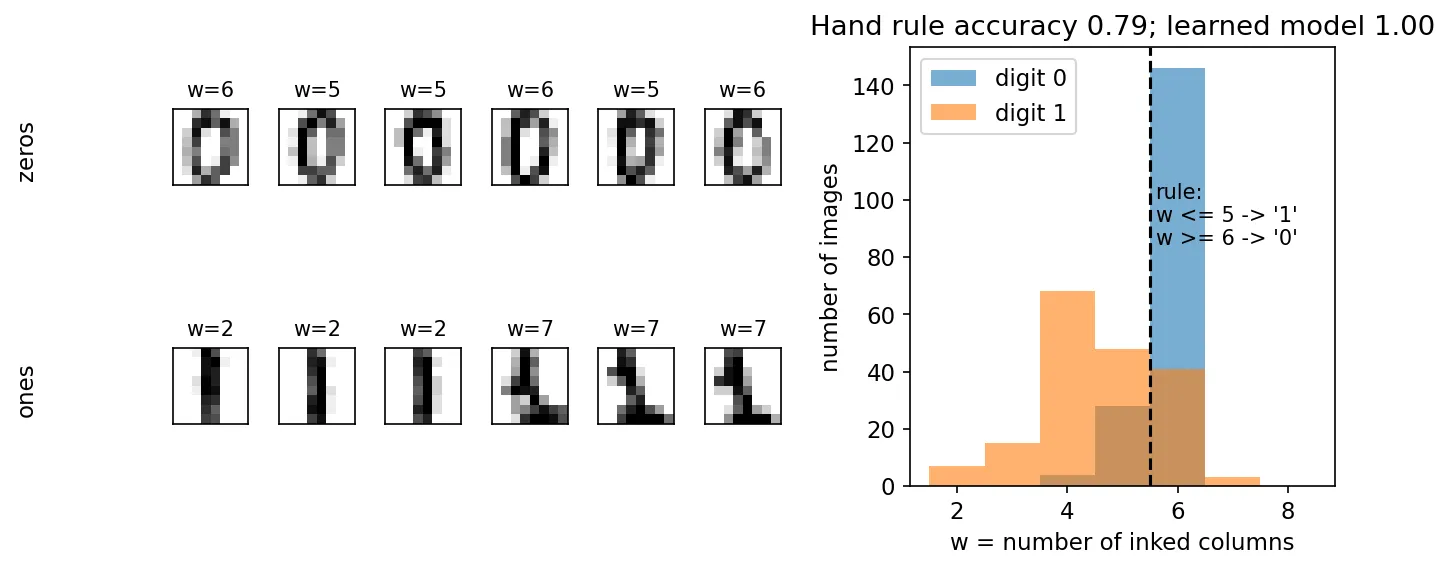

This small experiment contains the whole argument for machine learning. When the rule is hard to put into words but examples are cheap, learn the rule from examples. It also shows the price: the learned model is a list of 65 numbers that is much harder to read than “count the columns.”

The learning paradigms

Plain version. Learning problems differ mainly in what feedback the learner gets: the right answer for every example, no answers at all, answers it can manufacture from the data itself, or only an occasional score for how well it did.

Paradigm	What the data looks like	What is learned	Typical example
Supervised	pairs $(x, y)$: input and the “right answer”	a function from $x$ to $y$	digit image → digit label
Unsupervised	inputs $x$ only	structure: groups, directions, outliers	grouping similar digits
Self-supervised	inputs $x$ only, but part of $x$ is hidden and used as the target	a general-purpose representation	predicting a masked word or image patch
Reinforcement	an agent’s actions and the rewards they earn	a policy: which action to take in each situation	game playing, tuning chat models

My original notes listed the first, second and fourth; self-supervised learning has since become the main way large models are pre-trained, so it gets its own row [9], [10].

Supervised learning

In supervised learning, the learner is given the right answers. The data is a set of examples $\{(x^{(i)}, y^{(i)})\}_{i=1}^{m}$, where $x^{(i)}$ is an input, $y^{(i)}$ is the desired output (the label or target), and $m$ is the number of examples. The goal is a function $f$ such that $f(x)$ is close to $y$, also for new inputs not in the data. That last part, called generalization, is the real goal; memorizing the examples is easy.

Unsupervised learning

In unsupervised learning there are no answers, only inputs $\{x^{(i)}\}$. The goal is to find something interesting in the data: groups of similar examples, a compact description, or examples that do not fit. There is no single “correct” output, which makes these methods useful for exploration and harder to evaluate.

Self-supervised learning

Self-supervised learning uses unlabeled data but turns it into a supervised problem by hiding part of each example and asking the model to predict the hidden part. In text, hide a word and predict it from the rest of the sentence. In images, hide most of the patches and reconstruct them: masked autoencoders hide 75% of an image’s patches and train a network to fill them in [12]. LeCun and Misra describe self-supervised learning as a way for models to acquire broad background knowledge from raw observation, because the labels come for free [9].

The point is not the fill-in-the-blank task itself; it is that a model which can fill in blanks well must have learned a lot about the structure of the data. The learned internal representation can then be adapted to many other tasks with few labels. This is the recipe behind foundation models: models trained on broad data at scale (usually self-supervised) and then adapted to a wide range of downstream tasks [10]. GPT-3, trained simply to predict the next word on a large text corpus, was able to perform many language tasks from a few examples given in the prompt, without further training [11].

Reinforcement learning

In reinforcement learning (RL), an agent interacts with an environment. At each step it observes a state, chooses an action, and receives a reward (a number) and a new state. Nobody tells it the right action; it must discover which actions lead to high total reward over time, often when the reward arrives long after the action that earned it. What is learned is a policy, a rule for choosing actions in each state [8]. Samuel’s checkers player is an early example of this setting [2].

Today, RL is best known for tuning large language models. In reinforcement learning from human feedback (RLHF), as described by Ouyang et al. [13], a pre-trained language model is first fine-tuned on demonstrations written by people (supervised learning). People then rank several model answers to the same prompt, and a separate reward model is trained to predict those rankings. Finally, the language model is optimized with RL to produce answers that the reward model scores highly. The authors report that labelers preferred the outputs of their 1.3-billion-parameter tuned model over those of the 175-billion-parameter GPT-3 [13]. More recently, DeepSeek-R1 used large-scale RL with automatically checkable rewards (such as whether a math answer is correct) to improve step-by-step reasoning [14].

Notice that RLHF chains three paradigms: self-supervised pre-training, supervised fine-tuning, and reinforcement learning. Real systems mix paradigms freely; the table above is a map, not a set of walls.

Supervised learning: regression and classification

Plain version. Supervised learning comes in two main kinds. Regression predicts a number; classification predicts a category.

Regression

In regression the target $y$ is a real number, so there are infinitely many possible outputs. Examples: predicting a stock price, a student’s final grade from earlier test scores, or a person’s age from a face image. The last one shows that the input can be an image while the output is still a single number.

Classification

In classification the target is one of a small, fixed set of categories (classes). Examples: spam versus not spam (two classes, binary classification), the shape category of a face, or a tumor type such as benign, malignant type 1 or malignant type 2 (multi-class classification). Classes are names, not quantities: “class 2” is not twice “class 1”. A classifier usually outputs a probability for each class and then picks the most likely one.

from sklearn.datasets import make_regression, make_classification
from sklearn.linear_model import LinearRegression, LogisticRegression

# Regression: the target is a real number.
X_r, y_r = make_regression(n_samples=100, n_features=1, noise=10.0, random_state=0)
reg = LinearRegression().fit(X_r, y_r)
print(reg.predict(X_r[:3]).round(1), y_r[:3].round(1))   # numbers vs numbers

# Classification: the target is one of a few labels.
X_c, y_c = make_classification(n_samples=100, n_features=2, n_redundant=0,
                               n_clusters_per_class=1, random_state=0)
clf = LogisticRegression().fit(X_c, y_c)
print(clf.predict(X_c[:5]), y_c[:5])                     # labels vs labels
print(clf.predict_proba(X_c[:2]).round(3))               # class probabilities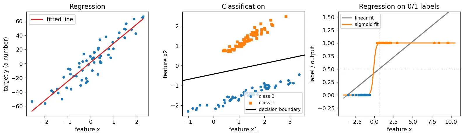

Why not use regression for classification?

It is tempting to code the classes as 0 and 1, fit a regression line, and call anything above 0.5 a 1. This can work on easy data, but it usually performs badly, for two reasons visible in Figure 2 (right). First, the line outputs values like $-0.4$ or $1.7$, which are not probabilities. Second, the squared error punishes a point that is correctly classified but far from the boundary, so a few extreme but easy examples pull the line and move its 0.5 crossing to the wrong place. Logistic regression (later in this tutorial) fixes both problems.

Unsupervised learning

Plain version. Without any answers, we can still ask: which examples belong together, how can each example be described with fewer numbers, and which examples are strange?

Clustering

Clustering groups similar examples. The classic algorithm is k-means [15]. Choose the number of groups $K$. Start with $K$ center points, then repeat two steps until nothing changes: assign each example to its nearest center, and move each center to the mean of the examples assigned to it. Each step can only lower the total squared distance from examples to their centers,

$$\sum_{i=1}^{m} \big\lVert x^{(i)} - \mu_{c^{(i)}} \big\rVert^2 ,$$

where $\mu_k$ is the center of cluster $k$ and $c^{(i)}$ is the cluster that example $i$ is assigned to. So the algorithm always stops, but possibly at a poor local solution, which is why it is run from several random starts. Jain’s review of fifty years of clustering research [15] stresses that there is no best clustering algorithm in general: the “right” groups depend on what similarity means for the data.

A common confusion: k-nearest neighbors (KNN) is not a clustering method. KNN classifies a new example by a vote among the $k$ most similar labeled training examples, so it is a supervised method [5]. The “k” in k-means counts clusters; the “k” in KNN counts neighbors.

Dimensionality reduction

Dimensionality reduction describes each example with fewer numbers while keeping as much useful information as possible. Principal component analysis (PCA) finds the directions along which the data varies most and projects the data onto the top few of them; the new coordinates are uncorrelated and successively capture as much variance as possible [16]. Two PCA coordinates can turn 64-pixel digit images into points on a plane that we can look at (Figure 3, middle).

Anomaly detection

Anomaly detection finds examples that do not fit the pattern of the rest: a fraudulent transaction, a defective part, a corrupted image. Chandola, Banerjee and Kumar’s survey [17] organizes the many techniques by the assumption each one makes about what “normal” looks like. A simple version uses PCA: fit a few components on the data, rebuild each example from them, and flag those with a large reconstruction error, because the components only describe what is common.

import numpy as np
from sklearn.datasets import load_digits
from sklearn.cluster import KMeans
from sklearn.decomposition import PCA

X, y = load_digits(return_X_y=True)             # y is used only to check, never to fit

# Clustering: ten groups, found without looking at y.
km = KMeans(n_clusters=10, n_init=10, random_state=0).fit(X)
purity = sum(np.bincount(y[km.labels_ == k]).max() for k in range(10)) / len(y)
print("cluster purity:", round(purity, 3))      # 0.792: most clusters are one digit

# Dimensionality reduction: 64 numbers per image -> 2 numbers.
Z = PCA(n_components=2).fit_transform(X)        # shape (1797, 2)

# Anomaly detection: images that a 20-component PCA rebuilds badly are unusual.
pca20 = PCA(n_components=20).fit(X)
err = ((X - pca20.inverse_transform(pca20.transform(X))) ** 2).sum(axis=1)
print("most unusual images:", np.argsort(err)[-5:])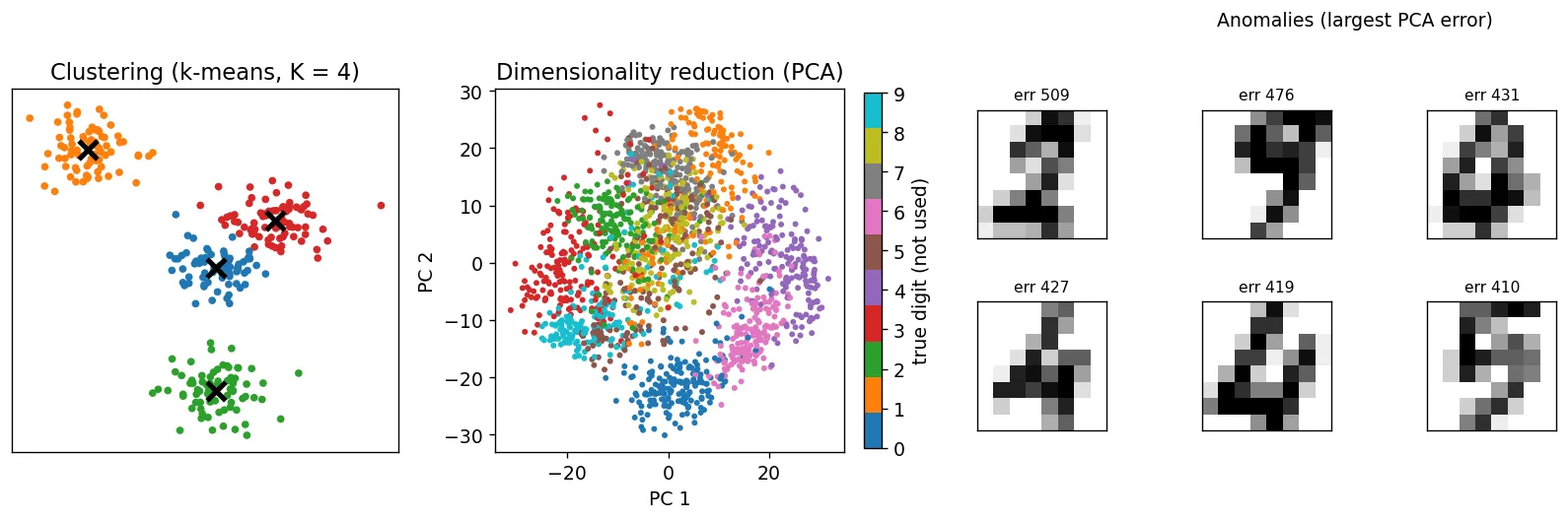

The purity check in the snippet uses the labels only after clustering, to see whether the discovered groups match the digits. About 79% of the images fall in a cluster dominated by their own digit, even though k-means never saw a label.

The vocabulary of a learning problem

Plain version. Before any math, we need names for the parts: what goes in, what comes out, what the right answer is, what the model is, and how we measure its mistakes.

Inputs, outputs and targets

• Features (inputs), $x$: the numbers that describe one example. For a digit image, the 64 pixel values; for a house, its size and number of rooms. With $n$ features we write $x = (x_1, \dots, x_n)$, and $x_j$ is the $j$-th feature.
• Target, $y$: the correct output, also called the label or ground truth. Only supervised learning has targets.
• Prediction, $\hat{y}$ (“y-hat”): what the model outputs for an input. The hat means “estimated”.
• Training example $i$: the pair $(x^{(i)}, y^{(i)})$. The superscript in parentheses is an index, not a power. $x_j^{(i)}$ is feature $j$ of example $i$.

The model and its parameters

The model is the function that maps features to a prediction. We write it $f_{w,b}$ to show that it depends on adjustable numbers called parameters, here $w$ (the weights) and $b$ (the bias):

$$\hat{y} = f_{w,b}(x).$$

Choosing the form of $f$ (a line, a curve, a neural network) is a design decision. Choosing the values of $w$ and $b$ is what learning does. Numbers we set by hand, such as the learning rate or polynomial degree, are called hyperparameters to distinguish them from the learned parameters.

Cost function

A loss $L(\hat{y}, y)$ measures how wrong one prediction is. The cost function $J(w, b)$ averages the loss over the training set, so it is a single number that says how wrong the whole model is for a given choice of parameters. The model is $f$; the cost is $J$. Keeping these two apart avoids a lot of confusion: $f_{w,b}(x)$ takes an input and returns a prediction, while $J(w, b)$ takes parameters and returns an error.

The objective of training is then precise: find the parameters that make $J$ as small as possible, so that $\hat{y}^{(i)}$ is close to $y^{(i)}$ for all training examples.

Training, validation and test sets

The data is split into three parts with different jobs:

• the training set is used to fit the parameters;
• the validation set is used during development to compare models and choose hyperparameters;
• the test set is used once, at the end, to estimate how the final model will do on new data.

The test set must not influence any decision, or the estimate becomes optimistic. We come back to why this split matters in the section on overfitting.

Linear regression

Plain version. Fit a straight line through the data. The line has two knobs: its slope and its height. Learning means turning the knobs until the line passes as close as possible to the points.

The model

With one feature, the linear regression model is

$$f_{w,b}(x) = w x + b,$$

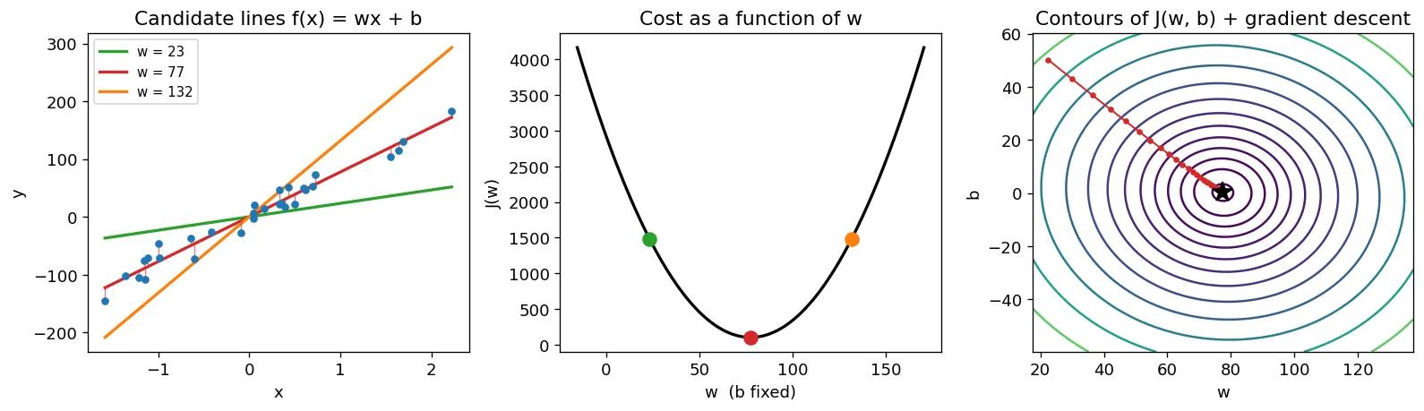
where $x$ is the feature, $w$ is the slope (how much the prediction changes when $x$ grows by 1) and $b$ is the intercept (the prediction when $x = 0$). Changing $w$ tilts the line; changing $b$ moves it up and down (Figure 4, left).

With $n$ features, the same model is a weighted sum,

$$f_{\mathbf{w},b}(\mathbf{x}) = \mathbf{w} \cdot \mathbf{x} + b = \sum_{j=1}^{n} w_j x_j + b,$$

where $\mathbf{w} = (w_1, \dots, w_n)$ holds one weight per feature. A common trick appends a constant feature $x_0 = 1$, so the bias becomes just another weight $w_0$ and the model shortens to $\mathbf{w} \cdot \mathbf{x}$. Either way, “linear” means linear in the parameters; we will later feed it squared or cubed features and it remains a linear regression.

The cost function: mean squared error

For each example, the error (residual) is $f_{w,b}(x^{(i)}) - y^{(i)}$. Squaring makes errors positive and punishes big ones more than small ones. Averaging over the $m$ training examples gives the mean squared error (MSE) cost:

$$J(w, b) = \frac{1}{2m} \sum_{i=1}^{m} \left( f_{w,b}(x^{(i)}) - y^{(i)} \right)^2 ,$$

where $m$ is the number of training examples and $(x^{(i)}, y^{(i)})$ is the $i$-th example. The extra factor $\tfrac{1}{2}$ is a convenience: it cancels the 2 that appears when we differentiate the square, and it does not change where the minimum is.

Picture the cost as a landscape over the parameters. If we fix $b$ and vary only $w$, $J$ is a parabola: lines that are too flat or too steep both have large error, and one slope in between is best (Figure 4, middle). With both $w$ and $b$, $J$ is a bowl, which we draw as a contour map of ellipses (Figure 4, right). The best line sits at the bottom of the bowl.

Why this bowl has one bottom

For linear regression, the MSE cost is a convex function of $(w, b)$: any straight segment between two points on its surface lies on or above the surface. A convex function has no separate local minima; every minimum is the global one. This is a special, friendly case. For many other models, including the neural networks of ML 02, the cost landscape has many valleys, and an optimizer can stop in one that is not the lowest. The original notes make exactly this point: in general, the best we can hope for is a good local minimum, close to the global one.

For linear regression we could even solve for the bottom directly with a formula (the normal equations, which np.polyfit uses). We use gradient descent anyway, because it is the method that still works when no formula exists.

Gradient descent

Plain version. Stand somewhere on the cost landscape in fog. Feel which way the ground slopes, take a small step downhill, and repeat. When the ground is flat, you are at the bottom.

The update rule

The derivative $\partial J / \partial w$ tells us how $J$ changes when $w$ increases a little: positive means “uphill to the right”, negative means “uphill to the left”. Its sign gives the direction, and its size says how steep the slope is. Gradient descent moves each parameter a small step against its derivative:

$$\begin{aligned} w &\leftarrow w - \alpha \frac{\partial J(w, b)}{\partial w}, \\ b &\leftarrow b - \alpha \frac{\partial J(w, b)}{\partial b}, \end{aligned}$$

where $\alpha > 0$ is the learning rate (step size) and $\leftarrow$ means “replace with”. Both derivatives are computed at the current $(w, b)$ before either is changed; this is called a simultaneous update. The vector of all partial derivatives is the gradient $\nabla J$, which points in the direction of steepest increase, so the update moves in the direction of steepest decrease [3].

For the MSE cost of linear regression, the chain rule gives

$$\frac{\partial J}{\partial w} = \frac{1}{m} \sum_{i=1}^{m} \left( f_{w,b}(x^{(i)}) - y^{(i)} \right) x^{(i)}, \qquad \frac{\partial J}{\partial b} = \frac{1}{m} \sum_{i=1}^{m} \left( f_{w,b}(x^{(i)}) - y^{(i)} \right).$$

Read them in words: the gradient for $w$ is the average error times the feature; the gradient for $b$ is the average error. If predictions are too high on average, $b$ goes down. If predictions are too high mainly where $x$ is large, $w$ goes down. With $n$ features, $\partial J / \partial w_j$ uses $x_j^{(i)}$ in place of $x^{(i)}$.

Implementing it from scratch

import numpy as np
from sklearn.datasets import make_regression

X, y = make_regression(n_samples=100, n_features=1, noise=10.0, random_state=0)
x = X[:, 0]                                   # one feature, shape (m,)
m = len(x)

def cost(w, b):
    return ((w * x + b - y) ** 2).sum() / (2 * m)

w, b, alpha = 0.0, 0.0, 0.1
for step in range(200):
    err = w * x + b - y                       # f_wb(x_i) - y_i for every i
    dj_dw = (err * x).sum() / m
    dj_db = err.sum() / m
    w, b = w - alpha * dj_dw, b - alpha * dj_db   # simultaneous update
    if step % 50 == 0:
        print(f"step {step:3d}  J = {cost(w, b):8.2f}")

print("gradient descent:", round(w, 3), round(b, 3))   # 42.619 -0.814
print("closed form     :", np.polyfit(x, y, 1).round(3))  # [42.619 -0.814]

The cost drops from about 800 to 57 within 50 steps and then stops changing. Gradient descent and the exact formula agree to three decimals. The remaining cost is not zero, because the data contains noise that no straight line can explain.

Convergence: where the derivative is zero

“Repeat until convergence” needs a definition. At a minimum, the landscape is flat, so the derivative is zero there, and the update $w - \alpha \cdot 0$ leaves $w$ unchanged. Note that it is the derivative, not the cost, that becomes zero: the cost at the minimum is just the smallest value available, 57 in the example above. In practice we stop when the cost decreases by less than a small tolerance between iterations, or when the gradient’s size falls below a threshold, or after a fixed budget of steps.

A useful consequence: as we approach a minimum, the derivative shrinks, so even with a fixed $\alpha$ the steps $\alpha\, \partial J/\partial w$ get smaller automatically. Gradient descent naturally slows down near the bottom.

Choosing the learning rate

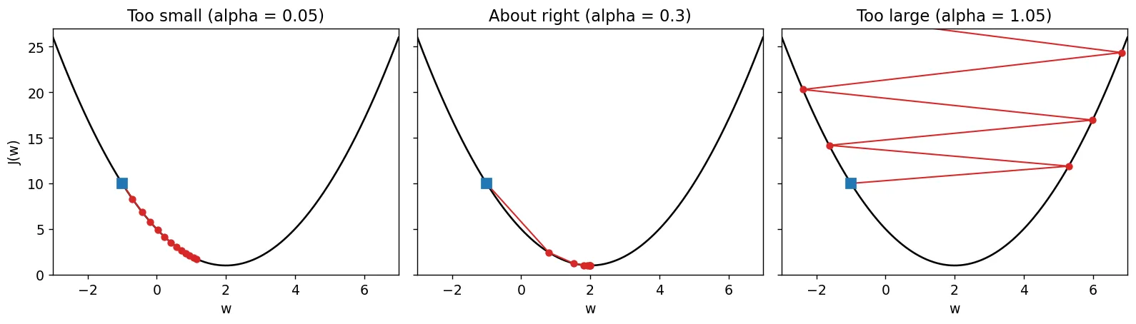
The learning rate is the most important hyperparameter of gradient descent (Figure 5):

• Too small: every step is tiny. The algorithm does go downhill, but it may need a very large number of steps.
• About right: the cost falls quickly and settles.
• Too large: a step jumps past the bottom to the other side of the valley, possibly higher than where it started. The parameters bounce back and forth, may never settle (overshoot), and can fly off to infinity (divergence).

The standard diagnostic is a learning curve: plot $J$ against the iteration number. With a good $\alpha$, $J$ decreases at every step. If $J$ ever goes up, $\alpha$ is too large (or there is a bug in the gradient). A practical recipe is to try values spaced by about a factor of 3, such as 0.001, 0.003, 0.01, 0.03, 0.1, 0.3, and pick the largest one whose curve decreases smoothly.

Many optimizers adapt the step size during training, either by a schedule that lowers $\alpha$ over time or by scaling each parameter’s step using running statistics of its past gradients, as Adam does [19]. These make “the steps become smaller near the minimum” an explicit design choice rather than just a side effect.

Batch, mini-batch and stochastic gradient descent

The gradient formula sums over all $m$ examples. That is fine for 100 examples and a problem for 100 million. The key insight, explained clearly in [3] and analyzed in depth by Bottou, Curtis and Nocedal [18], is that the gradient is an average, that is, an expectation over the data, and an average can be estimated from a sample.

• Batch gradient descent uses the whole training set for every update. Each step is exact and expensive.
• Mini-batch gradient descent shuffles the data and, for each update, uses a small random subset (a mini-batch) of $B$ examples, typically 32 to a few hundred. Each step is a noisy but unbiased estimate of the full gradient, and costs $B/m$ as much.
• Stochastic gradient descent (SGD), in the strict sense, uses one example per update ($B = 1$). In practice, “SGD” often refers to the mini-batch version too.

One full pass through the training data is an epoch. Beware of naming in code: the batch_size argument in deep-learning libraries means the mini-batch size, not the batch-gradient-descent “whole set”.

The noise in mini-batch gradients is not only tolerable but often helpful: in the same number of epochs, mini-batch descent makes many more updates than batch descent. Bottou et al. argue that this is why stochastic methods dominate large-scale learning: they reach a useful accuracy with far less computation than exact methods [18].

import numpy as np
from sklearn.datasets import make_regression

X, y = make_regression(n_samples=10_000, n_features=5, noise=10.0, random_state=0)
m, n = X.shape
rng = np.random.default_rng(0)

def minibatch_gd(batch_size, alpha=0.05, epochs=5):
    w, b = np.zeros(n), 0.0
    for epoch in range(epochs):
        order = rng.permutation(m)                    # shuffle once per epoch
        for start in range(0, m, batch_size):
            idx = order[start:start + batch_size]
            err = X[idx] @ w + b - y[idx]
            w -= alpha * X[idx].T @ err / len(idx)    # gradient estimated on the batch
            b -= alpha * err.mean()
    return ((X @ w + b - y) ** 2).mean() / 2

for bs in [m, 64, 1]:                                 # batch, mini-batch, stochastic
    print(f"batch size {bs:5d}: J = {minibatch_gd(bs, alpha=0.05 if bs > 1 else 0.005):.2f}")
# batch size 10000: J = 6127.00   (only 5 updates in 5 epochs)
# batch size    64: J = 49.93     (785 updates)
# batch size     1: J = 50.64     (50,000 noisy updates)

With the same five passes over the data, batch descent has made only five steps and is still far from the bottom, while mini-batch descent has essentially converged (the noise level of this data puts the best achievable $J$ near 50). Single-example SGD gets there too, but needs a smaller learning rate because its gradients are noisier, and it cannot use vectorized arithmetic efficiently.

Feature scaling

Plain version. If one feature is measured in thousands and another in fractions, the cost landscape becomes a long, narrow valley, and gradient descent zigzags. Putting all features on similar scales turns the valley into a round bowl that is easy to descend.

Why scale matters

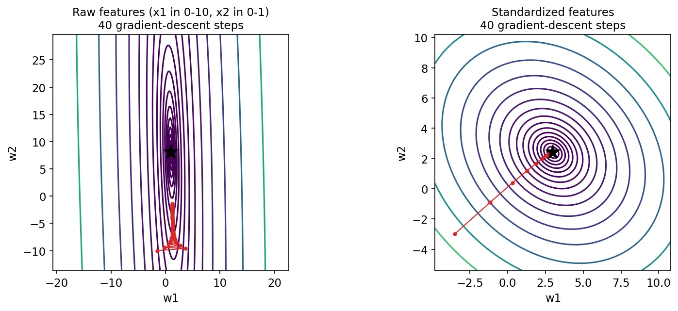
Suppose feature $x_1$ (say, house area in square feet) ranges over thousands and feature $x_2$ (number of bedrooms) ranges from 1 to 5. A small change in $w_1$ changes the predictions a lot; a similar change in $w_2$ barely matters. So $J$ is extremely steep along $w_1$ and very flat along $w_2$: the contours are thin ellipses. A learning rate small enough not to diverge along the steep direction makes almost no progress along the flat one (Figure 6, left).

Standardization and min–max scaling

The most common fix is standardization (z-score normalization):

$$x_j' = \frac{x_j - \mu_j}{\sigma_j},$$

where $\mu_j$ and $\sigma_j$ are the mean and standard deviation of feature $j$ computed on the training set. Each scaled feature then has mean 0 and standard deviation 1. An alternative is min–max scaling, $x_j' = (x_j - \min_j)/(\max_j - \min_j)$, which maps the training range to $[0, 1]$ and is the usual choice for pixel intensities (divide by 255 for 8-bit images). Both are available in scikit-learn as StandardScaler and MinMaxScaler [5].

Two rules prevent subtle bugs. Compute $\mu_j, \sigma_j$ on the training set only, then apply the same numbers to validation, test and future data. And remember that scaling changes the meaning of the learned weights: a weight now says how much the prediction changes per standard deviation of the feature.

import numpy as np
from sklearn.datasets import make_regression

X, y = make_regression(n_samples=200, n_features=2, noise=5.0, random_state=1)
X = X * np.array([1000.0, 1.0])               # feature 1 now has a ~1000x wider range

def gd(X, y, alpha, steps=500):
    m, n = X.shape
    w, b = np.zeros(n), 0.0
    for _ in range(steps):
        err = X @ w + b - y
        w -= alpha * X.T @ err / m
        b -= alpha * err.mean()
    return ((X @ w + b - y) ** 2).mean() / 2

print("raw,    alpha=1e-7:", round(gd(X, y, 1e-7), 2))    # 158.01; alpha=3e-6 diverges
mu, sigma = X.mean(axis=0), X.std(axis=0)
Xs = (X - mu) / sigma                          # z-score standardization
print("scaled, alpha=0.1 :", round(gd(Xs, y, 0.1), 2))    # 13.47

On the raw features, any learning rate above about $2 \times 10^{-6}$ diverges, and with a safe one the cost is still stuck near 158 after 500 steps (it is still near 158 after 5,000), because the second weight barely moves. After standardization, $\alpha = 0.1$ reaches the minimum (about 13, the noise level) easily.

Logistic regression for classification

Plain version. Keep the weighted sum from linear regression, but squash its output into the range 0 to 1 so it can be read as a probability. Then choose the weights so that the probability is high for the true class.

The sigmoid function

The sigmoid (logistic) function is

$$g(z) = \frac{1}{1 + e^{-z}},$$

where $z$ is any real number. It maps $-\infty$ to 0, $+\infty$ to 1 and $0$ to exactly $0.5$, with an S-shaped curve in between (Figure 7, left). It is also symmetric, $g(-z) = 1 - g(z)$, and has the convenient derivative $g'(z) = g(z)\,\big(1 - g(z)\big)$.

The model and the decision boundary

Logistic regression feeds the linear model into the sigmoid:

$$f_{\mathbf{w},b}(\mathbf{x}) = g(\mathbf{w} \cdot \mathbf{x} + b) = \frac{1}{1 + e^{-(\mathbf{w} \cdot \mathbf{x} + b)}},$$

and interprets the output as the estimated probability that the label is 1, $f_{\mathbf{w},b}(\mathbf{x}) = P(y = 1 \mid \mathbf{x})$. Despite the name, it is a classification method. To make a decision, predict 1 when this probability is at least 0.5. Since $g(z) \ge 0.5$ exactly when $z \ge 0$, the rule is

$$\hat{y} = 1 \quad \text{if} \quad \mathbf{w} \cdot \mathbf{x} + b \ge 0, \qquad \hat{y} = 0 \text{ otherwise}.$$

The set where $\mathbf{w} \cdot \mathbf{x} + b = 0$ is the decision boundary. With two features it is a straight line; in general it is a flat hyperplane, with $\mathbf{w}$ perpendicular to it. Points far from the boundary get probabilities near 0 or 1; points near it get probabilities near 0.5. To obtain a curved boundary, feed the model nonlinear features such as $x_1^2$ or $x_1 x_2$; the model stays linear in its parameters.

The cost: cross-entropy (log loss)

Why not reuse squared error? Combined with the sigmoid, the squared-error cost is not convex in $(\mathbf{w}, b)$: it develops flat plateaus and multiple valleys. Instead, logistic regression uses the log loss, also called binary cross-entropy:

$$L\big(f, y\big) = -\,y \log f \;-\; (1 - y) \log (1 - f),$$

where $f = f_{\mathbf{w},b}(\mathbf{x})$ is the predicted probability and $y \in \{0, 1\}$ is the true label. Only one of the two terms is active for each example. If $y = 1$, the loss is $-\log f$: zero when $f = 1$, and growing without bound as $f \to 0$. If $y = 0$, the loss is $-\log(1 - f)$, the mirror image (Figure 7, middle). Confident wrong answers are punished very heavily; confident right answers cost almost nothing.

The cost is the average over the training set:

$$J(\mathbf{w}, b) = \frac{1}{m} \sum_{i=1}^{m} \Big[ -\,y^{(i)} \log f_{\mathbf{w},b}(\mathbf{x}^{(i)}) - \big(1 - y^{(i)}\big) \log \big(1 - f_{\mathbf{w},b}(\mathbf{x}^{(i)})\big) \Big].$$

This choice is not arbitrary. If we treat each label as a coin flip with probability $f_{\mathbf{w},b}(\mathbf{x}^{(i)})$ of coming up 1, then $J$ is exactly the negative log-likelihood of the training labels, divided by $m$. Minimizing it is maximum likelihood estimation [3]. And with the sigmoid, this cost is convex, so gradient descent again finds the single global minimum.

Gradient descent, again

Using $g' = g(1 - g)$, the derivative of the log loss simplifies remarkably:

$$\frac{\partial J}{\partial w_j} = \frac{1}{m} \sum_{i=1}^{m} \left( f_{\mathbf{w},b}(\mathbf{x}^{(i)}) - y^{(i)} \right) x_j^{(i)}, \qquad \frac{\partial J}{\partial b} = \frac{1}{m} \sum_{i=1}^{m} \left( f_{\mathbf{w},b}(\mathbf{x}^{(i)}) - y^{(i)} \right).$$

This has exactly the same form as the linear-regression gradient: average error times feature. The only difference is inside $f$. This is not a coincidence; it holds for a whole family of models that pair an output function with its matching likelihood, and it is one reason gradient descent code is so reusable.

import numpy as np
from sklearn.datasets import make_classification

X, y = make_classification(n_samples=200, n_features=2, n_redundant=0,
                           n_clusters_per_class=1, class_sep=1.5, random_state=3)

def sigmoid(z):
    return 1.0 / (1.0 + np.exp(-z))

def log_loss(p, y, eps=1e-12):
    p = np.clip(p, eps, 1 - eps)              # avoid log(0)
    return -(y * np.log(p) + (1 - y) * np.log(1 - p)).mean()

w, b, alpha = np.zeros(2), 0.0, 0.5
for step in range(1000):
    p = sigmoid(X @ w + b)                    # predicted P(y = 1 | x)
    w -= alpha * X.T @ (p - y) / len(y)       # same form as linear regression
    b -= alpha * (p - y).mean()

p = sigmoid(X @ w + b)
print("log loss:", round(log_loss(p, y), 3))  # 0.06
print("accuracy:", ((p >= 0.5) == y).mean())  # 0.99
print("boundary: %.2f*x1 + %.2f*x2 + %.2f = 0" % (w[0], w[1], b))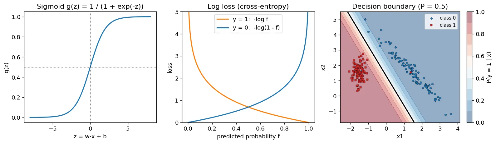

More than two classes

For $K > 2$ classes, the standard generalization gives each class its own weight vector and score $z_k = \mathbf{w}_k \cdot \mathbf{x} + b_k$, and turns the scores into probabilities that sum to 1 with the softmax function, $P(y = k \mid \mathbf{x}) = e^{z_k} / \sum_{l=1}^{K} e^{z_l}$. The cost is again the average negative log probability of the true class (categorical cross-entropy) [3]. This is what scikit-learn’s LogisticRegression did for the ten digits at the start of this tutorial, and it is exactly the output layer of most classification networks in ML 02.

Overfitting, underfitting and regularization

Plain version. A model that is too simple misses the pattern (underfitting). A model that is too flexible memorizes the training examples, noise included, and fails on new ones (overfitting). We detect the difference with data the model did not train on, and we tame an over-flexible model by penalizing large weights.

Seeing it happen

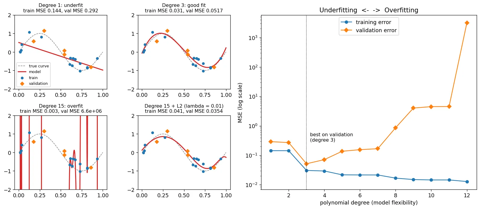
Take 25 noisy samples of a smooth curve and fit polynomials of different degrees, which is linear regression on the features $x, x^2, \dots, x^d$ (Figure 8):

• Degree 1 (underfitting, high bias). A straight line cannot follow the curve. The error is large on the training set and on new data.
• Degree 3 (a good fit). The curve follows the trend and ignores the noise. Errors are small on both.
• Degree 15 (overfitting, high variance). The curve passes almost exactly through every training point, so the training error is nearly zero. Between and beyond the points it swings wildly, and the error on new data explodes.

The training error alone cannot tell the good model from the overfitted one; it even prefers the overfitted one. Only data that the model did not see can reveal the difference. This is why we keep a validation set.

Using the validation and test sets

The workflow is:

1. Fit each candidate model (each degree, each regularization strength) on the training set.
2. Compare the candidates on the validation set and keep the best one.
3. Report the chosen model’s error on the test set, once.

Why three sets and not two? Because picking the best of many candidates on the validation set is itself a form of fitting: the winner is partly the one that got lucky on those particular examples. The untouched test set gives an unbiased final estimate. When data is scarce, cross-validation replaces the single validation set: split the training data into $k$ folds, train $k$ times, each time validating on a different fold, and average.

The pattern to look for: if training and validation errors are both high, the model underfits (use a more flexible model or better features). If training error is low but validation error is much higher, the model overfits (get more data, simplify the model, or regularize).

L2 regularization

Regularization keeps a flexible model but discourages extreme parameter values. The wild curve of the degree-15 fit needs huge, finely balanced weights. L2 regularization adds a penalty on the squared size of the weights to the cost:

$$J_{\text{reg}}(\mathbf{w}, b) = J(\mathbf{w}, b) + \frac{\lambda}{2m} \sum_{j=1}^{n} w_j^2 ,$$

where $J$ is the original cost (MSE or log loss), $\lambda \ge 0$ is the regularization strength (a hyperparameter), and the sum runs over the weights but conventionally not the bias $b$. With $\lambda = 0$ we recover the original model; as $\lambda$ grows, the weights are pulled toward zero and the fitted function becomes smoother; too large a $\lambda$ underfits. For linear regression, this is ridge regression, introduced by Hoerl and Kennard to stabilize least-squares estimates when features are strongly correlated [20].

The gradient-descent update shows what the penalty does:

$$w_j \leftarrow w_j \left(1 - \alpha \frac{\lambda}{m}\right) - \alpha \frac{\partial J}{\partial w_j}.$$

Before each ordinary step, every weight is multiplied by a number slightly less than 1. This is why L2 regularization is also called weight decay in neural-network training [3].

import numpy as np
from sklearn.model_selection import train_test_split
from sklearn.pipeline import make_pipeline
from sklearn.preprocessing import PolynomialFeatures, StandardScaler
from sklearn.linear_model import LinearRegression, Ridge
from sklearn.metrics import mean_squared_error

rng = np.random.default_rng(0)
x = rng.uniform(0, 1, 25)
y = np.sin(2 * np.pi * x) + rng.normal(0, 0.25, 25)      # true curve + noise
X = x[:, None]

# 60% train, 20% validation, 20% test
X_tmp, X_te, y_tmp, y_te = train_test_split(X, y, test_size=0.2, random_state=0)
X_tr, X_va, y_tr, y_va = train_test_split(X_tmp, y_tmp, test_size=0.25, random_state=0)

def fit(degree, lam=0.0):
    reg = Ridge(alpha=lam) if lam > 0 else LinearRegression()   # sklearn calls lambda "alpha"
    model = make_pipeline(PolynomialFeatures(degree), StandardScaler(), reg)
    return model.fit(X_tr, y_tr)

for degree, lam in [(1, 0), (3, 0), (15, 0), (15, 1e-2)]:
    model = fit(degree, lam)
    tr = mean_squared_error(y_tr, model.predict(X_tr))
    va = mean_squared_error(y_va, model.predict(X_va))
    print(f"degree {degree:2d}, lambda {lam:g}: train MSE {tr:.3f}, val MSE {va:.3g}")

best = fit(15, 1e-2)                                    # chosen on validation only
print("test MSE:", round(mean_squared_error(y_te, best.predict(X_te)), 3))

The output tells the whole story: degree 1 has train/validation MSE of 0.144/0.292 (underfit), degree 3 has 0.031/0.052 (good), and unregularized degree 15 has a training MSE of 0.003 but a validation MSE in the millions, because some validation points fall in wide gaps between training points (for example between $x \approx 0.27$ and $x \approx 0.61$), where the polynomial swings wildly. Adding a mild L2 penalty ($\lambda = 0.01$) to the same degree-15 model gives 0.041/0.035, and its test MSE is 0.075.

Evaluating a model

Plain version. A single number never tells the whole story. Choose a metric that matches what a mistake costs, and always compare against a trivial baseline.

Regression metrics

For regression, the most common metric is the MSE, $\frac{1}{m}\sum_i (\hat{y}^{(i)} - y^{(i)})^2$, here without the $\tfrac12$ that was only a training convenience. Its square root, the RMSE, is in the same units as $y$ and is easier to interpret (“off by about 3 points on average”). The mean absolute error, $\frac{1}{m}\sum_i |\hat{y}^{(i)} - y^{(i)}|$, is less sensitive to a few large errors [5].

Classification metrics

For classification, accuracy is the fraction of correct predictions. It is easy to understand and easy to be fooled by. In the digits data, about 10% of the images are 9s. A “model” that always answers “not a 9” is 90% accurate and completely useless.

The confusion matrix counts the four outcomes for a binary problem, with “positive” meaning the class we care about:

	predicted positive	predicted negative
actually positive	true positive (TP)	false negative (FN)
actually negative	false positive (FP)	true negative (TN)

From it,

$$\text{accuracy} = \frac{TP + TN}{TP + TN + FP + FN}, \qquad \text{precision} = \frac{TP}{TP + FP}, \qquad \text{recall} = \frac{TP}{TP + FN}.$$

Precision answers “when the model says positive, how often is it right?” Recall answers “of all the real positives, how many did the model find?” They trade off: lowering the 0.5 decision threshold of logistic regression finds more positives (higher recall) but raises more false alarms (lower precision). Which matters more depends on the cost of each mistake: a cancer screen should not miss tumors (high recall), while a spam filter should not hide real mail (high precision). The F1 score, the harmonic mean of precision and recall, combines both into one number [5].

import numpy as np
from sklearn.datasets import load_digits
from sklearn.model_selection import train_test_split
from sklearn.linear_model import LogisticRegression
from sklearn.metrics import confusion_matrix, accuracy_score, precision_score, recall_score

X, y = load_digits(return_X_y=True)
y = (y == 9).astype(int)                  # "is it a 9?": only about 10% positives
X_tr, X_te, y_tr, y_te = train_test_split(X, y, test_size=0.3, stratify=y, random_state=0)

lazy = np.zeros_like(y_te)                # always answers "not a 9"
model = LogisticRegression(max_iter=5000).fit(X_tr, y_tr)
pred = model.predict(X_te)

print("lazy accuracy :", round(accuracy_score(y_te, lazy), 3), " recall:", recall_score(y_te, lazy))
print("model accuracy:", round(accuracy_score(y_te, pred), 3),
      " precision:", round(precision_score(y_te, pred), 3),
      " recall:", round(recall_score(y_te, pred), 3))
print(confusion_matrix(y_te, pred))       # rows: true 0/1, columns: predicted 0/1
# lazy accuracy : 0.9   recall: 0.0
# model accuracy: 0.974  precision: 0.87  recall: 0.87

The lazy baseline reaches 90% accuracy with zero recall. The real model’s 97.4% accuracy sounds only a little better, but its recall of 0.87 shows that it actually finds most of the 9s. Always report the baseline, and always look past accuracy when classes are imbalanced. The same metrics reappear, with more care about thresholds and multiple classes, in the DIP chapter on pattern classification.

Modern view

The mechanics in this tutorial (a parameterized model, a cost, gradient-based optimization, and held-out evaluation) have not changed in decades, and every system discussed below still uses them. What has changed is where the features come from, where the labels come from, and how large the models are. A handful of reviews map these shifts well.

Machine learning as a field. Jordan and Mitchell’s review in Science [7] frames machine learning around a single question, how to build computers that improve automatically through experience, and places it at the intersection of computer science and statistics, at the core of artificial intelligence and data science. They attribute its rapid spread across science, medicine, manufacturing, education and finance to three things arriving together: new learning algorithms and theory, an explosion in the amount of available data, and cheap computation. That framing is a useful antidote to hype: the method is only as good as the data and the experience it is given.

From feature engineering to representation learning. For a long time, the success of a classical model depended mostly on hand-designed features, the “count the inked columns” step of Figure 1 done by experts: edge histograms, texture descriptors, keypoint descriptors (see DIP 12). Bengio, Courville and Vincent [21] argue that this dependence is a weakness, because the right representation is what makes a task easy or hard, and propose learning the representation itself from data. Their review covers the tools for this (probabilistic models, autoencoders, manifold learning and deep networks) and the general priors that make a representation good, such as disentangling the separate explanatory factors behind the data. In the language of this tutorial, a deep network is still “features followed by logistic regression”, except that the features are produced by earlier layers whose weights are learned by the same gradient descent. That is the subject of ML 02.

Self-supervised learning. Learning representations needs data, and labels are the expensive part. Jing and Tian’s survey of self-supervised visual feature learning [22] sorts the label-free “pretext tasks” into four families: generation-based (for example, reconstructing or colorizing images), context-based (exploiting spatial or temporal structure, such as the arrangement of image patches), free-semantic-label-based (using labels that come automatically, for example from rendering engines or classical methods), and cross-modal (checking whether two signals, such as video and audio, belong together). It also sets out the evaluation protocol that is still standard: judge a representation by how well it transfers to downstream tasks such as classification, detection and segmentation. The later survey by Gui et al. [23] reorganizes the field around context-based methods, contrastive learning (with negative examples, self-distillation, or feature decorrelation), generative methods dominated by masked image modeling, and hybrids of contrastive and generative objectives, reflecting the shift toward masked prediction after masked autoencoders [12]. For practitioners, Balestriero et al.’s Cookbook of Self-Supervised Learning [24] groups modern methods into a deep metric learning family, a self-distillation family, a canonical correlation analysis family and masked image modeling, and is candid about how much the outcome depends on details such as data augmentation and the small “projector” network used during training.

Foundation models. The report by Bommasani et al. [10] named the resulting paradigm: models trained on broad data at scale, usually self-supervised, then adapted to many downstream tasks. It highlights two consequences. Emergence: capabilities such as following instructions from a few examples in the prompt [11] appear with scale rather than being designed in. Homogenization: many applications are now adapted from the same few base models, which gives great leverage but means that a defect in the base model is inherited by everything built on it. The report also stresses how limited our understanding is of how these models work and when they fail.

Reinforcement learning from human feedback. RL has moved from games to the final stage of training language models [13], [14]. Casper et al. [25] survey what can go wrong. They follow the three steps of RLHF (collecting human feedback, fitting a reward model, and optimizing the policy) and catalog problems at each: feedback from people is noisy, inconsistent and can be manipulated; a reward model is only an imperfect proxy for what people want; and a policy optimized hard against that proxy can exploit its errors. They separate problems that better methods within RLHF could solve from fundamental limitations that would require a different approach, and they argue for transparency and for combining RLHF with other safety measures rather than relying on it alone.

Optimization at scale. Bottou, Curtis and Nocedal [18] explain why the humble stochastic gradient method, and not more sophisticated optimizers from classical numerical analysis, became the workhorse of machine learning: when data is plentiful, a cheap noisy step beats an expensive exact one. Adaptive methods such as Adam [19] add per-parameter step sizes on top. Every model mentioned in this section, however large, is trained with a descendant of the mini-batch loop in this tutorial.

Open problems. Despite the scale, several questions from this beginner’s tutorial remain the hard ones. Generalization: very large models fit their training data almost perfectly yet still generalize, which does not match the simple overfitting picture of Figure 8, and why this happens is not fully understood. Evaluation: when a model is trained on a large fraction of the public internet, it is hard to guarantee that the test set was not in the training data, so a clean train/test separation, the foundation of honest evaluation, is difficult to verify. Objectives: the cost function is the only thing the model optimizes, and RLHF shows how hard it is to write a cost that captures what people actually want. And data: what a model learns is bounded by the data and labels it sees, with all their gaps and biases.

For computer vision specifically, the classical route (hand-made features plus a simple classifier) is developed in the DIP chapter on pattern classification, and the learned route continues in ML 02 and Deep Learning for Image Processing.

Key takeaways

• Machine learning replaces hand-written rules with a flexible model whose parameters are fitted to examples; it shines when the rule is hard to state but examples are easy to get.
• The paradigms differ in feedback: supervised (right answers; regression for numbers, classification for categories), unsupervised (no answers; clustering, dimensionality reduction, anomaly detection), self-supervised (answers made from the data itself), and reinforcement learning (rewards for actions). KNN is supervised; k-means is clustering.
• Keep the model $f_{w,b}(x)$ and the cost $J(w,b)$ apart: the model maps inputs to predictions; the cost maps parameters to an error. Training means minimizing $J$.
• Gradient descent repeats $w \leftarrow w - \alpha\, \partial J / \partial w$. At a minimum the derivative is zero. The learning rate must be small enough to avoid overshooting and large enough to make progress; mini-batches make each step cheap.
• Scale features before gradient descent, using statistics from the training set only.
• Logistic regression applies a sigmoid to a linear score and minimizes cross-entropy; its decision boundary is $\mathbf{w}\cdot\mathbf{x} + b = 0$, and its gradient has the same form as linear regression’s.
• Judge models on data they did not train on: choose with the validation set, report once on the test set, regularize (L2) when the model overfits, and look beyond accuracy when classes are imbalanced.

Exercises

1. A derivative by hand. For the one-feature MSE cost $J(w, b) = \frac{1}{2m}\sum_i (wx^{(i)} + b - y^{(i)})^2$, derive $\partial J/\partial w$ and $\partial J/\partial b$. Then, for the three points $(1, 2), (2, 4), (3, 6)$ starting at $w = 0, b = 0$, compute one gradient-descent step with $\alpha = 0.1$.

Hint

The chain rule on each square gives $2(wx^{(i)} + b - y^{(i)}) \cdot x^{(i)}$, and the 2 cancels the $\tfrac12$, giving the formulas in the gradient-descent section. At $w = b = 0$ the errors are $-2, -4, -6$. So $\partial J/\partial w = (-2 \cdot 1 - 4 \cdot 2 - 6 \cdot 3)/3 = -28/3$ and $\partial J/\partial b = -12/3 = -4$. After one step, $w = 0.1 \cdot 28/3 \approx 0.933$ and $b = 0.4$.

2. Find the divergence threshold. For $J(w) = \frac{1}{2m}\sum_i (wx^{(i)} - y^{(i)})^2$ (no bias), show that one gradient step multiplies the distance to the optimum $w^\ast$ by $1 - \alpha s$, where $s = \frac{1}{m}\sum_i (x^{(i)})^2$. For which $\alpha$ does gradient descent converge? Check your answer with the gd function from the feature-scaling section.

Hint

$\partial J/\partial w = s\,(w - w^\ast)$ because $J$ is a parabola with curvature $s$ and minimum at $w^\ast$. So $w_{\text{new}} - w^\ast = (1 - \alpha s)(w - w^\ast)$. It converges when $|1 - \alpha s| \lt 1$, that is $0 \lt \alpha \lt 2/s$; at $\alpha = 1/s$ it lands on the minimum in one step. With several features, $s$ is replaced by the largest eigenvalue of $\frac{1}{m}X^\top X$, which is why one huge-scale feature forces a tiny $\alpha$.

3. Regression for classification. Generate 1-D data with make_classification(n_features=1, n_informative=1, n_redundant=0, n_clusters_per_class=1), then add five extra examples of class 1 with very large $x$. Fit both LinearRegression (thresholding at 0.5) and LogisticRegression. Compare their accuracy before and after adding the extra points, and explain the difference.

Hint

The extra points are easy to classify, but the squared error still wants the line to pass near them. The line’s slope drops, its 0.5 crossing moves toward class 1, and some ordinary class-1 points near the boundary become misclassified. The log loss of a correctly classified, far-away point is already close to 0, so logistic regression barely moves.

4. Scaling the digits. Train the from-scratch logistic regression of this tutorial on “9 versus not 9” with the digits data, once on raw pixels (0 to 16) and once on pixels divided by 16. Use the same number of steps and find the largest learning rate that works for each. Does scaling change the final accuracy, the speed, or both?

Hint

All pixels share one unit here, so the effect is milder than in Figure 6, but the raw inputs are 16 times larger, which multiplies the gradient’s size and the landscape’s curvature. The safe learning rate on raw pixels is roughly $16^2 = 256$ times smaller. With properly tuned learning rates, both reach similar accuracy; the scaled version is simply easier to tune.

5. Choosing lambda. Using the polynomial example, fix degree 15 and try $\lambda \in \{10^{-6}, 10^{-4}, 10^{-2}, 1, 100\}$. Plot training and validation MSE against $\lambda$ on a log axis. Which end underfits, which overfits, and which $\lambda$ would you pick? Why must you not use the test set to make this choice?

Hint

Tiny $\lambda$ behaves like no regularization (overfitting: low training error, high validation error). Huge $\lambda$ flattens the curve toward a constant (underfitting: both errors high). Pick the $\lambda$ with the lowest validation error. If the test set guided the choice, it would no longer be an unbiased estimate of performance on new data.

6. Which paradigm? Classify each problem as supervised (regression or classification), unsupervised, self-supervised or reinforcement learning, and name the target or reward: (a) estimating the remaining battery life of a phone from usage logs with recorded outcomes; (b) grouping a million unlabeled product photos for browsing; (c) pre-training an image model by predicting the missing quarter of each photo; (d) teaching a robot arm to stack blocks with a score given only when the stack stands; (e) flagging unusual readings in a factory sensor stream with no labeled failures.

Hint

(a) Supervised regression; target: remaining hours. (b) Unsupervised clustering. (c) Self-supervised; the target is the hidden pixels, made from the data itself. (d) Reinforcement learning; reward: whether the stack stands, delayed until the end. (e) Unsupervised anomaly detection.

References

1. Shyandram, “Introduction to Machine Learning,” blog post, 2024; updated 2026. link
2. A. L. Samuel, “Some studies in machine learning using the game of checkers,” IBM Journal of Research and Development, vol. 3, no. 3, pp. 210–229, 1959. doi
3. I. Goodfellow, Y. Bengio and A. Courville, Deep Learning, MIT Press, 2016. book site
4. A. Ng, E. Shyu, A. Bagul and G. Ladwig, “Machine Learning Specialization,” DeepLearning.AI and Stanford Online, Coursera. course page
5. F. Pedregosa, G. Varoquaux, A. Gramfort, V. Michel, B. Thirion et al., “Scikit-learn: Machine learning in Python,” Journal of Machine Learning Research, vol. 12, pp. 2825–2830, 2011. link
6. E. Alpaydin and C. Kaynak, “Optical Recognition of Handwritten Digits,” UCI Machine Learning Repository, 1998. doi
7. M. I. Jordan and T. M. Mitchell, “Machine learning: Trends, perspectives, and prospects,” Science, vol. 349, no. 6245, pp. 255–260, 2015. doi
8. R. S. Sutton and A. G. Barto, Reinforcement Learning: An Introduction, 2nd ed., MIT Press, 2018. book page
9. Y. LeCun and I. Misra, “Self-supervised learning: The dark matter of intelligence,” Meta AI blog, 2021. link
10. R. Bommasani, D. A. Hudson, E. Adeli et al., “On the opportunities and risks of foundation models,” arXiv:2108.07258, 2021. arXiv
11. T. Brown, B. Mann, N. Ryder, M. Subbiah, J. D. Kaplan et al., “Language models are few-shot learners,” in Advances in Neural Information Processing Systems (NeurIPS), vol. 33, 2020. link
12. K. He, X. Chen, S. Xie, Y. Li, P. Dollár and R. Girshick, “Masked autoencoders are scalable vision learners,” in Proc. IEEE/CVF Conference on Computer Vision and Pattern Recognition (CVPR), pp. 15979–15988, 2022. arXiv
13. L. Ouyang, J. Wu, X. Jiang, D. Almeida, C. Wainwright et al., “Training language models to follow instructions with human feedback,” in Advances in Neural Information Processing Systems (NeurIPS), vol. 35, 2022. link
14. DeepSeek-AI, “DeepSeek-R1: Incentivizing reasoning capability in LLMs via reinforcement learning,” Nature, vol. 645, pp. 633–638, 2025. arXiv
15. A. K. Jain, “Data clustering: 50 years beyond K-means,” Pattern Recognition Letters, vol. 31, no. 8, pp. 651–666, 2010. doi
16. I. T. Jolliffe and J. Cadima, “Principal component analysis: A review and recent developments,” Philosophical Transactions of the Royal Society A, vol. 374, no. 2065, 20150202, 2016. doi
17. V. Chandola, A. Banerjee and V. Kumar, “Anomaly detection: A survey,” ACM Computing Surveys, vol. 41, no. 3, 2009. doi
18. L. Bottou, F. E. Curtis and J. Nocedal, “Optimization methods for large-scale machine learning,” SIAM Review, vol. 60, no. 2, pp. 223–311, 2018. doi
19. D. P. Kingma and J. Ba, “Adam: A method for stochastic optimization,” in Proc. International Conference on Learning Representations (ICLR), 2015. arXiv
20. A. E. Hoerl and R. W. Kennard, “Ridge regression: Biased estimation for nonorthogonal problems,” Technometrics, vol. 12, no. 1, pp. 55–67, 1970. doi
21. Y. Bengio, A. Courville and P. Vincent, “Representation learning: A review and new perspectives,” IEEE Transactions on Pattern Analysis and Machine Intelligence, vol. 35, no. 8, pp. 1798–1828, 2013. doi
22. L. Jing and Y. Tian, “Self-supervised visual feature learning with deep neural networks: A survey,” IEEE Transactions on Pattern Analysis and Machine Intelligence, vol. 43, no. 11, pp. 4037–4058, 2021. doi
23. J. Gui, T. Chen, J. Zhang, Q. Cao, Z. Sun, H. Luo and D. Tao, “A survey on self-supervised learning: Algorithms, applications, and future trends,” arXiv:2301.05712, 2023. arXiv
24. R. Balestriero, M. Ibrahim, V. Sobal, A. Morcos, S. Shekhar et al., “A cookbook of self-supervised learning,” arXiv:2304.12210, 2023. arXiv
25. S. Casper, X. Davies, C. Shi et al., “Open problems and fundamental limitations of reinforcement learning from human feedback,” Transactions on Machine Learning Research, 2023. TMLR · arXiv