OPT 01 · Modeling Decisions and Convex Sets
Needs: ML 01A · Linear Algebra for Learning, ML 01C · Numerical Computation and Gradient Checks
Navigate: this page and this track: Navigate: this page and this track
On this page
- What you’ll learn1 min
- The big picture1 min
- From a sentence to an optimization model3 min
- Feasibility and optimal value2 min
- Affine and convex sets2 min
- Convex hulls and relaxations1 min
- A working vocabulary of convex sets2 min
- Operations that preserve convexity2 min
- Projections and separating hyperplanes2 min
- Interior, relative interior and hidden equalities1 min
- Convexity of a problem requires both sets and functions2 min
- Modern view1 min
- Key takeaways1 min
- Exercises1 min
- References
Optimization
Explore this chapter 1 interactive experiment
Place two feasible points on a circle, slide along the segment between them, and compare a disk with an annulus.
What you’ll learn
- Translate a decision into variables, an objective, constraints and fixed data.
- Distinguish feasible, optimal, infeasible, unbounded and unattained problems.
- Understand affine sets, convex combinations, convex hulls and cones.
- Recognize halfspaces, polyhedra, norm balls, ellipsoids and positive-semidefinite cones.
- Use convexity-preserving operations, projections and separating hyperplanes.
- Check what a numerical solution establishes about the model and the underlying application.
The big picture
An image restoration system must choose pixel values. A scheduler must choose resource allocations. A fitting procedure must choose coefficients. In each case there are many possible choices, a way to compare them, and restrictions on what choices are allowed. Optimization makes those three ingredients explicit.
This course follows Stephen Boyd and Lieven Vandenberghe’s Convex Optimization [1]. Its emphasis is learning to recognize, formulate and solve problems whose geometry supports global guarantees. The first chapters develop sets, functions, standard problem forms and duality. Applications connect that theory to fitting, statistical estimation and geometric design. The final chapters examine numerical algorithms and modern extensions.
The analogy is deliberately limited: taste need not be a convex function, and real ingredients can come in indivisible packages. The first skill is to identify which parts of a real decision fit a convex model and which parts do not. A convincing model is more valuable than a fast solver applied to the wrong equations.
Convex optimization is also useful around nonconvex learning. It can solve a linear classifier on fixed features, compute a constrained prediction, fit a calibration curve or construct a lower bound for a harder problem. It does not turn an arbitrary neural network’s training objective into a convex one. The guarantees belong to the particular mathematical problem being solved.
From a sentence to an optimization model
Plain version. Decide what you can change, what is already known, what makes a choice good, and which rules it must obey. Write these down before choosing an algorithm.
A general scalar optimization problem can be expressed as
Here is the vector of decision variables; is the scalar objective to minimize; are inequality constraint functions; and are equality constraint functions. Fixed measurements and design parameters enter these functions but are not decision variables unless the model explicitly makes them so.
For example, suppose two operations use amounts and of a shared resource. A capacity constraint might be , while rules out negative allocations. If the target allocation is , an objective prefers choices close to that target. The numbers in this example specify a synthetic model; they are not measurements of a production system.
Units are part of the formulation. Adding a cost in dollars to a reconstruction error in intensity units requires a weighting convention. A coefficient that converts between their scales should be interpreted and tested. Changing image normalization from zero-to-255 to zero-to-one can change the effective regularization if other terms are left unchanged.
It is helpful to keep a small modeling ledger: each variable’s meaning and unit, each fixed input’s provenance, the justification for each constraint, and the interpretation of the objective. This avoids treating a convenient formula as if it were the only possible representation of the task.
Constraints and penalties express different commitments
A hard constraint says a choice is disallowed. A penalty says a violation or deviation is undesirable but can be exchanged against other benefits. The distinction matters even if both produce similar answers on one example.
Consider nonnegative image intensities. Enforcing makes all feasible outputs nonnegative. Adding a quadratic penalty on negative entries may still permit some negativity if it improves the data term enough. Increasing a penalty is not automatically the same as enforcing an exact constraint, especially with finite numerical precision.
Likewise, a budget constraint sets a fixed resource limit. A cost penalty expresses a preference that depends on the tradeoff coefficient. Choosing that coefficient is part of the application, not something convexity decides. Later chapters derive how dual multipliers quantify the sensitivity to changing hard constraints.
Worked model: a target allocation under a capacity limit
A target need not obey the available capacity. Optimization finds the nearest allowed allocation, rather than reducing every coordinate by the same amount.
Take the synthetic target and minimize with and . The target uses nine units of capacity, so it is infeasible. At the solution the capacity boundary is active. Its normal is , so the shortest correction points along :
Here is the candidate allocation, is the correction scale, and is the capacity normal. Substituting gives and both coordinates are positive, so the nonnegativity constraints do not alter this projection.
Why is this the closest point? For any feasible , . Expand the objective difference:
Here is any feasible competitor; all other symbols are defined above. Both terms are nonnegative. The candidate therefore minimizes the objective globally, whose value is . This calculation connects the variables, the active rule, the correction direction and the optimum before introducing a solver [1].
Feasibility and optimal value
Plain version. An allowed answer and the best allowed answer are different objects. Sometimes there are no allowed answers; sometimes the model prefers choices that run away without bound.
The feasible set is
Here is the set of points satisfying all constraints and function-domain restrictions. A point in is feasible. The optimal value is
is the greatest lower bound on achievable objective values. An optimizer is a feasible point attaining that value: . The infimum can exist without an optimizer.
Four cases are worth distinguishing. A feasible problem can have an attained finite optimum. An infeasible problem has an empty feasible set. An unbounded-below problem has objective values tending to negative infinity. An unattained problem can have a finite limiting value that no feasible point reaches.
For a concrete unattained example, minimize subject to . The optimal value is zero, but zero is excluded. For an unbounded example, minimize on . For an infeasible example, require both and . These have very different implications even if a solver returns no finite optimizer.
Closedness and boundedness help establish existence. A continuous objective on a nonempty compact feasible set attains a minimum. A closed but unbounded set can also admit a minimizer if the objective grows sufficiently at infinity. The existence question concerns the model before any algorithm starts.
Numerical status is evidence about a finite-precision computation
A solver typically assesses constraint residuals, optimality conditions or a primal–dual gap against tolerances. A successful status does not imply exact real-number feasibility. It also does not establish that the measurements, objective or application constraints were correct.
If the application requires a genuinely safe limit, decide how numerical tolerances relate to that limit. Rescaling a constraint can change its raw residual without changing the feasible set. For example, and are equivalent mathematically but have very different unnormalized residual magnitudes.
Record the scale, tolerance and units of residuals. Do not compare objective values between runs whose objective definitions differ. If an algorithm stops because iterations are exhausted, report that condition rather than interpreting a nearly unchanged iterate as a proof of optimality.
Affine and convex sets
Plain version. An affine set contains complete lines through its points. A convex set only needs to contain the line segments between its points.
For points and scalar , a two-point affine combination is
Here and are vectors, is their combination, and controls position along their line. Allowing every real traces the entire line. Restricting traces the segment between the endpoints.
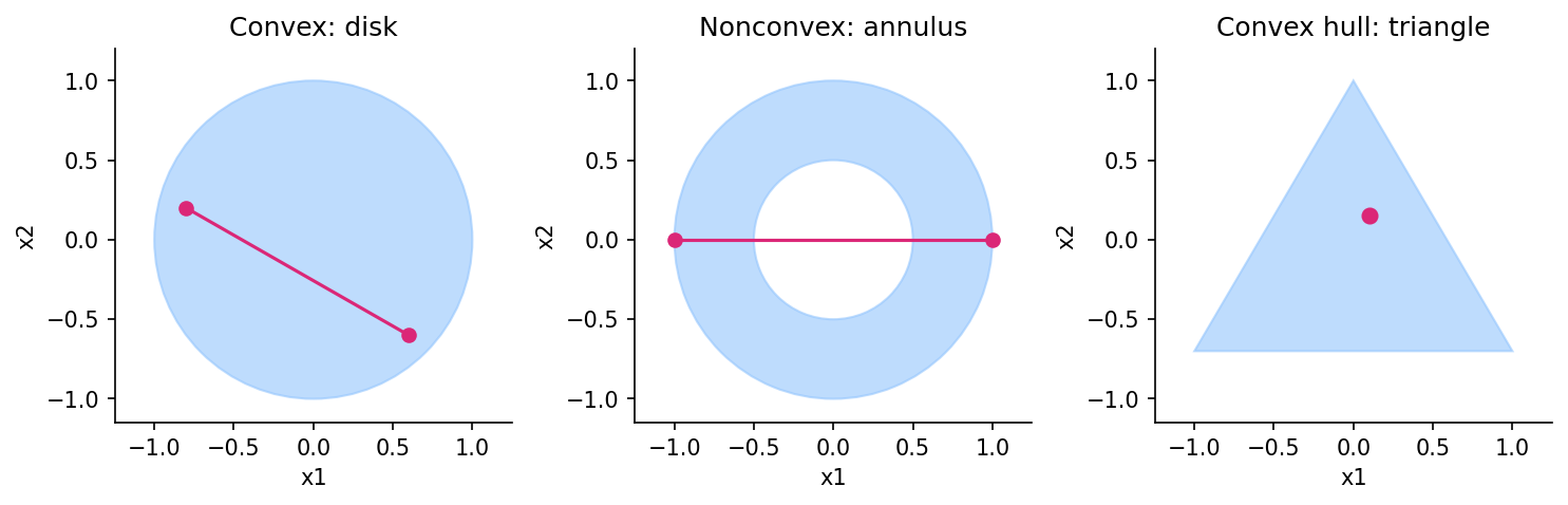
A set is affine if it contains all affine combinations of its points. It is convex if it contains all convex combinations, where coefficients are nonnegative and sum to one. Thus every affine set is convex, while a disk is convex without being affine.
For finitely many points the convex-combination rule is
are the endpoint vectors and are their weights. The combination is a weighted average. Nonnegative weights are essential: extrapolation can leave a convex set.
Convexity says nothing by itself about smooth boundaries, boundedness or closedness. An open ball is convex; a line is unbounded and convex; a single point is convex. The empty set is conventionally convex because there are no endpoint pairs violating the definition.
A counterexample disproves; sampled tests do not prove
To disprove convexity, find two points in the set whose midpoint or another segment point lies outside. This is often simpler than analyzing a complicated boundary. A ring fails because opposite points average to its excluded center.
To prove convexity, use the definition or a preservation rule. Testing many random pairs can reveal a bug but cannot establish the property for every pair. A tiny nonconvex notch may escape all sampled checks.
The distinction is similar to numerical gradient checks. They are valuable implementation diagnostics, while the mathematical argument addresses a universal statement. Use both for different purposes, and label their roles clearly.
Code: combinations and a nonconvex counterexample
This self-contained NumPy example verifies particular points. The mathematical proof for the disk follows from the triangle inequality, not from the assertions alone.
Code · Python · 12 lines
import numpy as np

u = np.array([0.8, 0.1])
v = np.array([-0.2, 0.7])
theta = np.linspace(0, 1, 101)
segment = theta[:, None] * u + (1 - theta[:, None]) * v
assert np.linalg.norm(segment, axis=1).max() <= 1 + 1e-12
ring_u, ring_v = np.array([1.0, 0.0]), np.array([-1.0, 0.0])
midpoint = (ring_u + ring_v) / 2
assert not (0.5 <= np.linalg.norm(midpoint) <= 1.2)
print("disk sampled-segment maximum norm:", np.linalg.norm(segment, axis=1).max())
print("ring midpoint:", midpoint, "norm:", np.linalg.norm(midpoint))
Convex hulls and relaxations
Plain version. A convex hull fills in every weighted average of a collection of choices. It is useful when discrete choices are hard, but its added points may be unavailable in the original application.
The convex hull of a set is
Here is the original collection; is the number of selected points in a finite combination; and is the smallest convex set containing all of .
Suppose an allocation must choose one of three configurations. The convex hull also permits mixtures. If mixtures correspond to time sharing, these points may be operationally meaningful. If the decision must select a single indivisible machine, a fractional hull point is a relaxation, not a feasible original answer.
For a minimization problem, enlarging the feasible set cannot increase the optimal value. Therefore a convex relaxation can provide a lower bound on a discrete problem. Turning its optimizer into an actual discrete choice requires another step, and the resulting rounded choice may violate constraints or lose objective quality.
Do not describe an exact optimum of the relaxed problem as an exact optimum of the original problem. Keep the original feasible set, relaxed set, relaxed lower bound and achieved original objective separate. The applications chapter returns to this distinction.
A working vocabulary of convex sets
Plain version. Most useful convex models are assembled from a few reusable geometric shapes. Learning those shapes makes an unfamiliar equation easier to classify.
Hyperplanes, halfspaces and polyhedra
A hyperplane and a closed halfspace have forms
is a point, is a nonzero normal vector and is an offset. A hyperplane is affine. A halfspace contains points on one side and its boundary.
A polyhedron is an intersection of finitely many halfspaces and hyperplanes, often written . Matrices hold constraint coefficients; vectors hold bounds. The inequality is componentwise. Polyhedra can be bounded, unbounded, lower-dimensional or empty.
A box is a polyhedron with coordinate bounds. A probability simplex adds nonnegativity and a sum-to-one equality. These forms show why probability vectors and bounded pixel values frequently fit convex constraints.
Norm balls and ellipsoids
A norm ball is
is its center, is its radius and is a norm. Norm triangle inequalities imply convexity. Different norms encode different geometry: a Euclidean ball is round, an infinity-norm ball is a box, and a one-norm ball has corners.
An ellipsoid can be written
is a matrix mapping the unit Euclidean ball, is the auxiliary ball coordinate and is the center. If is invertible, an equivalent quadratic description uses a positive-definite shape matrix. Singular produces a lower-dimensional image, which remains convex.
Cones and matrix inequalities
A convex cone is closed under nonnegative combinations:
is the cone, are its points and are nonnegative scalars. The weights do not have to sum to one. The nonnegative orthant is a simple example.
The second-order cone consists of pairs satisfying , where is scalar and is a vector. It represents many norm constraints.
The positive-semidefinite cone contains symmetric matrices satisfying
is symmetric, and is an arbitrary test vector. This condition is written . It is not the same as requiring every matrix entry to be nonnegative. Covariance matrices naturally lie in this cone.
Generalized inequalities use a cone to define order: means . For the orthant this becomes coordinatewise order; for symmetric matrices it becomes positive-semidefinite order. Stating the cone avoids confusing these different comparisons.
Operations that preserve convexity
Plain version. Once a set is known to be convex, certain operations create another convex set automatically. These rules are stronger and easier to reuse than repeated plotting.
Intersections of convex sets are convex. A point on the segment between two members remains in every set being intersected. This is why combining convex constraints is straightforward.
Affine images and inverse images preserve convexity. If is convex, both the transformed set and the set are convex. Here is a fixed matrix and a fixed vector. Nonlinear transformations do not have this general guarantee.
Cartesian products and sums of convex sets are convex. Projection onto selected coordinates is an affine image, so eliminating auxiliary variables preserves convexity of the feasible set. This fact underlies many extended formulations: a model may be easier to express with extra variables.
Unions are usually not convex. Two disjoint balls illustrate the failure. Replacing “and” with “or” in a constraint specification can fundamentally change the problem, even when each branch is individually convex.
For matrix variables, the same reasoning works in a vector space of symmetric matrices. If and are positive semidefinite, then is positive semidefinite for : test the quadratic form against every vector.
Two short proofs you can reuse
Convexity proofs usually track a segment through the construction. Suppose , where are convex. For , the mixture belongs to each set, hence to their intersection. The same argument works for any collection of convex sets.
For an affine image, let and with . Their mixture is
Here is convex, are fixed transformation data, and are image points. The bracketed point belongs to , so the mixture belongs to the image. This is why eliminating auxiliary coordinates preserves a convex feasible set [1, Section 2.3].
The corresponding union proof fails: two endpoints can come from different sets. For instance, and , but their midpoint zero lies in neither interval. Each interval is convex; the union is not. In modeling language, simultaneous convex rules preserve convexity, while an either-or choice can break it.
Projections and separating hyperplanes
Plain version. Projection finds the closest allowed point to an arbitrary point. The direction from that point toward its projection also reveals which side of a boundary contains the feasible set.
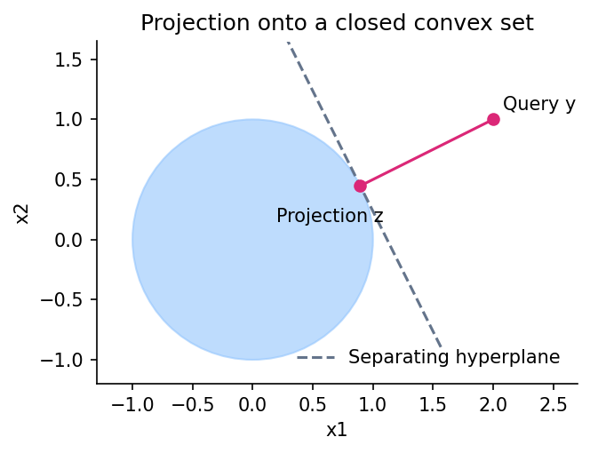
For a nonempty closed convex set , Euclidean projection is
is the query point, is the candidate feasible point and is the unique minimizing point. Strict convexity of squared Euclidean distance ensures uniqueness. Other distances or nonconvex sets need not have the same property.
Let . Its optimality condition is
Here is the projection and ranges over feasible points. The condition follows by considering a small step from toward any and requiring that squared distance cannot decrease.
If , the vector is nonzero. It defines a hyperplane through with the entire feasible set on the opposite side from . This is a concrete separating-hyperplane construction.
More general separation theorems compare disjoint convex sets [1, Section 2.5]. Separation need not have a positive margin without additional assumptions. Closedness, compactness and distance between sets matter when asserting strict separation.
Code: box and ball projections
Projection onto a box clips each coordinate. Projection onto a Euclidean ball rescales a point only if it lies outside. These formulas follow from the geometry and are covered by the geometric applications in [1, Section 8.1].
Code · Python · 15 lines
import numpy as np

y = np.array([2.0, -1.5])
lower, upper = np.array([0.0, -1.0]), np.array([1.0, 1.0])
box_projection = np.clip(y, lower, upper)
radius = 1.0
ball_projection = y * min(1.0, radius / np.linalg.norm(y))
rng = np.random.default_rng(2)
points = rng.normal(size=(1000, 2))
points /= np.maximum(1.0, np.linalg.norm(points, axis=1))[:, None]
inequality = (points - ball_projection) @ (y - ball_projection)
assert inequality.max() <= 1e-12
assert np.all(box_projection >= lower) and np.all(box_projection <= upper)
print("box projection:", box_projection)
print("ball projection:", ball_projection)
The sampled check illustrates the projection inequality. It does not replace a proof for all feasible points. More complicated projections can themselves require solving an optimization problem; “projected gradient” does not imply that projection is inexpensive.
Deriving the projection test
The projection inequality comes from trying every feasible direction, not from drawing a tangent that looks right. Let and choose any . Convexity makes feasible for . Because minimizes squared distance, its one-sided directional derivative must be nonnegative:
Here is the query, its projection, a feasible comparison point and the segment parameter. This gives the stated separation inequality. It is also sufficient: expanding the distance at yields the distance at , plus a nonnegative inner product and .
Uniqueness follows just as directly. If distinct both minimized squared distance, their midpoint would be feasible and have a strictly smaller value. Closedness supplies existence: a minimizing sequence stays in a bounded distance sublevel set and has a convergent subsequence whose limit remains in . Thus nonempty, closed and convex each plays a specific role [1].
Interior, relative interior and hidden equalities
Plain version. A feasible set can have room to move within its own plane even if it has no room to move in the full surrounding space.
Consider probability vectors whose coordinates sum to one. They lie in a hyperplane, so their ordinary interior in the full vector space is empty. They can nevertheless have strictly positive coordinates and an interior relative to that hyperplane.
The affine hull is the smallest affine set containing . The relative interior is the interior measured within that affine hull. This distinction matters in feasibility conditions and duality. Requiring a full-dimensional interior would incorrectly exclude many useful equality-constrained models.
Equality constraints can also be hidden inside inequalities. If both and are present, they force equality. Recognizing such structure can improve interpretation and numerical treatment.
Strict feasibility does not mean the same thing as having a small computed violation. It is a mathematical property requiring relevant inequalities to hold strictly while equalities remain satisfied. The duality and interior-point chapters specify exactly when this condition is needed.
Convexity of a problem requires both sets and functions
Plain version. Convex allowed choices are only half of the story. The objective must also have the right shape, and equality constraints must preserve that geometry.
A convex minimization problem uses a convex objective, convex inequality functions and affine equalities on their appropriate domains [1]. The next chapter defines convex functions and proves the rules used to recognize them.
A convex feasible set alone does not guarantee a convex optimization problem. Minimizing a function with many valleys over a box remains nonconvex. Conversely, a convex objective with disconnected discrete constraints remains nonconvex.
When the whole problem is convex, every local minimizer is global. This does not guarantee a unique minimizer: a linear objective can be constant along an entire face. Stronger objective properties, such as strict convexity on the feasible set, can establish uniqueness when a minimum exists.
Neither globality nor uniqueness guarantees numerical ease at every scale. A huge dense problem may require more memory than available. An extremely ill-conditioned model may be difficult at tight tolerance. Convexity supplies structural advantages, while complexity and implementation still matter.
Why a local minimum must be global
Convexity excludes a better distant answer by connecting it to the current point. Suppose is a local minimizer of convex on convex feasible set , but some feasible has . For any , define . Then
Here is a feasible segment point and its mixing weight. For arbitrarily small positive , the point lies arbitrarily close to and improves the objective, contradicting local minimality. No differentiability is needed [1].
This proof gives globality, not uniqueness. For example, minimizing on gives every point as a global minimizer. Adding a strictly convex objective makes distinct tied minimizers impossible, because their feasible midpoint would have lower cost. Existence remains separate: minimizing on is convex but has no minimizer.
These three questions guide solver expectations. Convexity makes local minima global; strict curvature can select one answer; closedness and objective growth can ensure an answer exists. A numerical procedure needs an appropriate convergence argument in addition to all three.
Modern view
Plain version. Modern convex optimization still begins with modeling and geometry. Recent methods change how a feasible set is accessed and how much computation is spent obtaining an accurate certificate.
Grant, Boyd and Ye’s disciplined convex programming framework [2] organizes models through verified composition rules. It is a modeling methodology, not an independent guarantee that any convenient expression is convex. An algebraically convex expression may need reformulation so its convexity is visible to the rule system.
Pokutta’s 2024 survey of Frank–Wolfe methods [3] distinguishes access through projection, barrier functions or a linear minimization oracle. Its useful lesson here is geometric: a feasible set that is easy to describe may still be expensive to project onto. Linear minimization can sometimes be cheaper, and convex combinations preserve feasibility. Later algorithm chapters explain those updates and their assumptions.
The PDLP report by Applegate and colleagues [4], first posted in 2025 and revised in 2026, develops a practical first-order linear-programming solver. It connects a primal–dual formulation with scaling, restarts and feasibility polishing. This is an original solver study, not a survey. We use it as evidence that implementation details and the desired accuracy remain important even for a familiar convex problem class.
Current challenges include representing complex constraints without excessive auxiliary structure, exploiting sparse matrices, making tolerances meaningful under scaling, and maintaining certificates when models are embedded in larger pipelines. A learned feature extractor can be nonconvex while a subsequent allocation problem is convex; describe each stage’s guarantees separately.
These sources are a curated reading path, not a claim that every optimization survey has been reviewed. The core theory in this course follows [1], while the modern sections identify precisely which extensions each source supports.
Key takeaways
- Variables, fixed data, objectives, constraints and units must be explicit.
- Feasibility, boundedness, attainment and numerical termination are different questions.
- Convex sets contain all weighted averages with nonnegative weights summing to one.
- Affine sets, polyhedra, norm balls and important cones provide reusable building blocks.
- Intersections and affine transformations preserve convexity; unions generally do not.
- Projection onto a closed convex set is unique and supplies a useful geometric certificate.
- Convex optimization guarantees concern the formulated problem and its stated assumptions.
Exercises
- Formulate allocating three nonnegative resources under a total budget, with squared deviation from a chosen target. State all units and distinguish variables from data.
Hint
Use a vector , nonnegativity, one sum constraint and a fixed target vector.
- Prove directly that the intersection of two convex sets is convex. Give a counterexample for their union.
Hint
A segment stays in both sets; two separated intervals disprove the union rule.
- A system can select one of three configurations. Explain when a convex mixture is an actual operational choice and when it is only a relaxation.
Hint
Consider time sharing versus an indivisible hardware choice.
- Derive projection onto a centered Euclidean ball. Identify what happens when the query point is already inside.
Hint
Outside the ball, the closest point lies on the query’s radial direction.
- Give a finite-valued convex problem whose optimum is not attained, and explain which existence condition fails.
Hint
An open interval can exclude its limiting optimum.
- A solver reports constraint residual . Explain why its adequacy cannot be judged without constraint scale and application units.
Hint
Rescaling the same inequality changes the raw residual.
References
- Stephen Boyd and Lieven Vandenberghe, Convex Optimization, Cambridge University Press, 2004. Reading: Chapters 1–2; Sections 4.1–4.2 and 8.1 for problem terminology and projections. Official book page, free official PDF.
- Michael Grant, Stephen Boyd and Yinyu Ye, “Disciplined Convex Programming,” in Global Optimization: From Theory to Implementation, Springer, 2006. Author’s publication page.
- Sebastian Pokutta, “The Frank-Wolfe Algorithm: A Short Introduction,” Jahresbericht der Deutschen Mathematiker-Vereinigung, 126, 2024. Open-access survey.
- David Applegate, Mateo Díaz, Oliver Hinder, Haihao Lu, Miles Lubin, Brendan O’Donoghue and Warren Schudy, “PDLP: A Practical First-Order Method for Large-Scale Linear Programming,” arXiv preprint, 2025, revised 2026. Verified paper record.
Check your understanding
This tutorial has 6 exercises. Can you solve them without opening the hints?
Go to the exercises ↑Next OPT 02 · Convex Functions, Composition and Conjugates · 18 min