OPT 08 · Geometric Applications, Splitting and Modern Methods
Needs: OPT 07 · Equality Constraints and Interior-Point Methods
Navigate: this page and this track: Navigate: this page and this track
On this page
- What you’ll learn1 min
- The big picture1 min
- 1. Distances, projections and separation1 min
- 2. Centers, ellipsoids and placement2 min
- 3. Relaxations are models with an explicit interpretation1 min
- 4. Proximal operations handle nonsmooth structure2 min
- 5. Split a signal model into simple subproblems3 min
- 6. Conditional gradients use a linear oracle2 min
- 7. Choose a method by structure, accuracy and information2 min
- 8. A complete convex-optimization capstone1 min
- Modern view3 min
- Key takeaways1 min
- Exercises1 min
- References
Optimization
Explore this chapter 1 interactive experiment
Compare soft thresholding with ordinary shrinkage and inspect its nonsmooth objective.
What you’ll learn
- Model distances, centers, separation and placement using convex geometry.
- Distinguish a convex application model from a relaxation of a discrete or nonconvex problem.
- Derive proximal updates for nonsmooth terms and constraints.
- Implement splitting for synthetic signal denoising and conditional gradients on a simplex.
- Choose methods by their expensive operations and check appropriate convergence evidence.
- Build a reproducible optimization capstone and connect it to modern surveys and methods.
The big picture
Convex optimization becomes useful when a problem’s structure tells you both how to model it and how to solve it. A geometric model may make projections simple. A signal model may separate a smooth data term from a nonsmooth prior. A distributed model may make local solves cheap while communication is expensive. The right algorithm works with that structure rather than hiding it.
The geometric reading follows Boyd and Vandenberghe’s Chapter 8, with modeling and approximation connections to Chapters 4 and 6 [1]. The algorithmic extensions use Parikh and Boyd’s proximal survey [2], Boyd et al.’s ADMM review [3], Condat et al.’s splitting survey [4] and Pokutta’s conditional-gradient introduction [5]. The chapter closes the track by connecting these operations to a complete modeling, solving and validation workflow.
All experiments use synthetic data and run locally on a CPU. Their purpose is to expose the objective, assumptions, residuals and failure modes. A smaller numerical objective is meaningful only after the feasible set, data scale and evaluation protocol have been checked.
1. Distances, projections and separation
A distance problem asks how close a point or set can get to another while obeying its restrictions. A projection finds the nearest allowed point. These geometric operations become building blocks for both applications and optimization algorithms.
For a nonempty closed convex set , define
Here is a fixed query point; is the optimization variable; is Euclidean norm; and is the projection. The objective is strictly convex in , so the minimizer is unique. Closedness ensures attainment; nonemptiness ensures the problem has a feasible point.
For a box, projection clips each coordinate to its interval. For an affine set, it solves a constrained quadratic. For a positive-semidefinite matrix cone, a projection involves the spectrum of a symmetric matrix. These are all convex projections, but their costs differ substantially. “Projected gradient” is a useful name only after the projection cost is understood.
A projection satisfies for every , where . The inequality says that the displacement from the projection to the query points away from every feasible direction. It supplies an optimality check and, when the query lies outside the set, a separating hyperplane.
Distances between two convex sets can be modeled by minimizing with and , where is a second set. The norm is convex in the pair. A finite infimum need not be attained for arbitrary unbounded sets; verify existence before interpreting an algorithm’s iterates as converging to a closest pair. For compact sets, the geometry is simpler.
Classification by separation also has a geometric interpretation. A linear score places a hyperplane between classes, where is its normal and its offset. Margin constraints can be convex when the data and labels are fixed. Choosing a representation jointly with all classifier parameters can create a different, nonconvex learning problem. The Pattern Recognition track develops the statistical context of these models.
2. Centers, ellipsoids and placement
A center can mean several different things. The center minimizing maximum distance to observations differs from the center of the largest ball fitting inside a feasible region. The analytic center of an inequality representation is another object. State the geometry before calling a point “the center.”
For a polyhedron described by , the largest contained Euclidean ball has center and radius obtained from
Here and are fixed inequality data; and are variables. The worst displacement of length at most in direction contributes . Every constraint is affine in because the normal vectors are fixed.
This center balances distance to boundaries in Euclidean units. Multiplying an inequality by a positive constant scales both its normal norm and right-hand side, preserving the geometric condition. A zero normal needs separate inspection: its inequality is either always satisfied or impossible. Do not divide by its norm blindly.
An ellipsoid allows different radii in different directions. Write it as , where is a positive-definite symmetric shape matrix, is the center and is an auxiliary unit-ball coordinate. Containment in a halfspace becomes . Maximizing models maximum volume up to an additive constant [1]. The domain is essential.
Centering and enclosing are different constraints. An inscribed ellipsoid must stay inside a region, while an enclosing ellipsoid must contain given points. Their convenient convex parameterizations differ. A visually plausible shape matrix can lead to a nonconvex formulation if inverses and variable products are introduced carelessly. Trace each transformation to its domain and convexity rule.
Placement problems often minimize sums of distances between movable points and fixed anchors. If connectivity and constraints are fixed, Euclidean norms yield a convex objective. Choosing which connections exist introduces discrete variables. Floorplanning can be convex after selecting a relative ordering of rectangles, but unknown nonoverlap choices contain disjunctions. The original physical problem and a convex subproblem need separate labels.
Worked center: a rectangle has more than one answer
The largest inscribed ball need not have a unique center. Take the rectangle , . The ball constraints reduce to and , with .
Here is the center and its radius. The shorter side forces . At maximum radius one, every center with is optimal. The problem is convex, yet its optimizer is not unique. The symmetric center is one valid answer, rather than a uniquely implied one.
For an inscribed ellipsoid, a symmetric positive-definite maps the unit ball to the shape. Its volume is the unit-ball volume multiplied by , because a linear map scales volume by its determinant. Maximizing therefore preserves volume maximizers. The containment rule follows by maximizing over , producing . This combines the support-function calculation of OPT 03 with the matrix curvature of OPT 02 [1, Chapter 8].
The convex formulation minimizes over the containment constraints. The halfspace normals are fixed, so the norm term is convex in . Allowing to become singular would leave the finite log-determinant domain and collapse the ellipsoid’s volume.
3. Relaxations are models with an explicit interpretation
A relaxation enlarges the feasible set to make a hard problem easier. It can produce a useful bound or a candidate that later needs rounding. A fractional solution is implementable only when the application permits mixtures, sharing or time allocation.
Suppose a binary configuration variable must lie in . Replacing that constraint by is a convex relaxation of the discrete requirement when the remaining formulation is convex. For minimization, enlarging the feasible set can only decrease the optimum, so the relaxed value is a lower bound on the original optimum. The bound does not mean the relaxed point is a valid discrete decision.
After rounding, evaluate the original objective and constraints again. Independent coordinate rounding can violate a total budget, a connectivity requirement or an equality. A repaired feasible rounded solution gives an upper bound; the relaxed optimum gives a lower bound. Their difference is meaningful when both values refer to the same original objective and the lower value is the exact relaxed optimum or a certified dual or error-corrected bound. An approximate relaxed primal objective alone is generally an upper bound on the relaxed optimum; it need not be a lower bound on the original discrete optimum.
The same care applies to convex surrogates in vision and learning. A norm penalty can encourage sparsity without solving a general count-minimization problem exactly. A convex data term may be a deliberate approximation to a physical measurement process. State whether the model is a statistical estimator, a computational relaxation or an exact reformulation. These purposes support different claims.
Parameter selection also belongs outside the numerical certificate. Solving a regularized problem to high accuracy does not prove that its regularization strength predicts well on new data. Select the strength using a valid validation protocol, then test once on held-out data. Keep numerical optimization error separate from model-selection and generalization error.
4. Proximal operations handle nonsmooth structure
A nonsmooth term need not be approximated by a steep smooth function. A proximal operation balances that term against staying near a proposed point. Many penalties and constraints admit a simple closed-form operation, making them suitable for first-order methods [2].
For a proper closed convex function and step scale , define
Here is the proposed point; is the subproblem variable; is allowed to take positive infinity to encode restrictions; and scales the quadratic proximity term. Under the stated conditions the subproblem has a unique minimizer.
For the indicator of a closed convex set, the proximal operation is projection. For , with , it is coordinatewise soft thresholding: . Here indexes coordinates. The operation can create exact zeros; ordinary gradient descent on the absolute-value penalty is undefined at zero.
To minimize with differentiable convex , proximal gradient takes
Here is the iteration index; is the smooth gradient; and is a step size selected to meet the method’s assumptions. If the gradient is -Lipschitz, a conservative fixed choice is . The constant bounds gradient variation, rather than the objective value itself.
For constrained least squares, this update becomes gradient followed by projection. For sparse least squares, it becomes gradient followed by soft thresholding. More complicated compositions, such as a nonsmooth function applied to a linear difference operator, may make the direct proximal map expensive. Splitting introduces auxiliary variables to keep the cheap operations separate.
A useful residual is the scaled update . Here is a proximal-gradient mapping. A zero mapping satisfies the first-order optimality condition for this convex composite problem. Its magnitude is a convergence diagnostic; interpret it together with scale, feasibility and an objective bound where available.
Derive soft thresholding at the corner
The proximal map solves the nonsmooth corner exactly. For one coordinate, minimize with and . The optimality condition is
Here is the proposed coordinate, the output and the absolute-value subdifferential. For , it equals one, so , valid only if . For , it equals minus one, giving , valid only if . At zero, the subdifferential is , so zero is optimal precisely when [2].
These three cases give the threshold formula. For the synthetic vector and threshold , the output is . A nonzero input can become exactly zero because zero has a whole interval of supporting slopes.
The proximal-gradient update follows by minimizing a local upper model of the smooth term: replace by and retain exactly. Completing the square centers this model at . Thus the method uses a gradient step for the smooth cost and an exact small solve for the nonsmooth cost. When , the smoothness inequality makes this model an upper bound, explaining the conservative step condition.
5. Split a signal model into simple subproblems
Piecewise-constant signals can be estimated by balancing agreement with observations against neighboring differences. A quadratic data term discourages large corrections; an absolute-difference penalty encourages many neighboring values to match. The resulting convex estimator is useful for a controlled denoising experiment, with behavior different from uniform smoothing.
Let contain noisy observations and compute adjacent differences. Solve
Here is the estimated signal and is the regularization strength. This is one-dimensional total-variation regularization as treated in proximal and splitting references [2–4]. The term describes local variation; it does not assert that every real signal is piecewise constant.
Introduce and apply the alternating direction method of multipliers, or ADMM [3]. In scaled form,
Here is the penalty parameter; is the identity matrix; is the scaled dual variable; and shrink denotes coordinatewise soft thresholding defined above. The inverse notation describes the solution mathematically; the implementation uses a factorization and solve. The split equality is satisfied at convergence, rather than necessarily at each intermediate iterate.
Code · Python · 28 lines
import numpy as np
from scipy.linalg import cho_factor, cho_solve

rng = np.random.default_rng(8)
n = 48
clean = np.r_[np.zeros(16), np.ones(16), np.full(16, 0.3)]
y = clean + rng.normal(0, 0.16, n)
D = np.diff(np.eye(n), axis=0)
lam, rho = 0.4, 4.0
factor = cho_factor(np.eye(n) + rho*D.T @ D)
x, z, u = y.copy(), np.zeros(n-1), np.zeros(n-1)
for k in range(2000):
    x = cho_solve(factor, y + rho*D.T @ (z-u))
    z_old = z.copy()
    v = D @ x + u
    z = np.sign(v) * np.maximum(np.abs(v)-lam/rho, 0)
    u += D @ x-z
    primal = np.linalg.norm(D @ x-z)
    dual = rho*np.linalg.norm(D.T @ (z-z_old))
    if max(primal, dual) < 1e-7:
        break
objective = lambda a: 0.5*np.sum((a-y)**2) + lam*np.abs(D @ a).sum()
print("Iterations and residuals:", k+1, primal, dual)
print("Objectives, raw and estimated:", objective(y), objective(x))
print("Synthetic MSE, raw and estimated:", np.mean((y-clean)**2), np.mean((x-clean)**2))
assert max(primal, dual) < 1e-7
assert objective(x) <= objective(y) + 1e-8
assert np.mean((x-clean)**2) < np.mean((y-clean)**2)
The last assertion checks this specific synthetic example; it is not a theorem that regularization always improves reconstruction. Strong regularization can flatten a real edge or remove a narrow peak. The objective chooses a compromise under the model, while clean-signal error requires ground truth that a real deployment may not have.
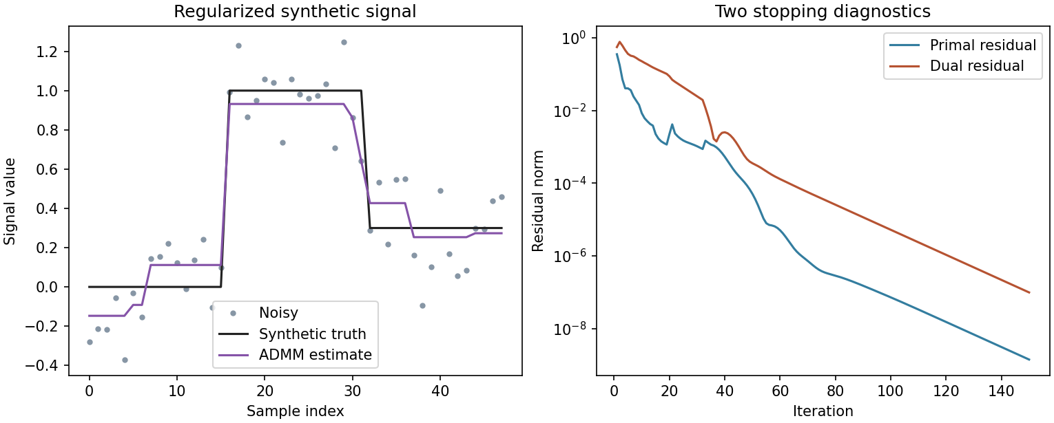
The factorization is reused because and are fixed. Changing the regularization strength only changes thresholding; changing changes the linear system and requires refactorization. If changes while retaining the same unscaled multiplier, rescale consistently. Otherwise the update silently changes the dual state.
For images, adjacent differences become horizontal and vertical operators, and the penalty can combine them in different ways. Boundary conditions and pixel scale affect the estimator. This chapter’s one-dimensional result cannot be reported as an image-restoration benchmark. Use Image Processing for measurement models and Deep Learning for Computer Vision for learned restoration comparisons.
Derive the split updates and their residuals
The ADMM equations come from retaining an explicit difference variable rather than taking a difficult composite proximal map. With , form the scaled augmented objective
Here is the signal, the observations, the difference matrix, the split differences, the scaled multiplier, and the penalty. The last term is constant during the primal subproblems. Differentiating in yields . Minimizing in is the soft-threshold problem centered at with threshold . The multiplier update then accumulates the split-equality error [3].
Why monitor two residuals? The primal residual checks the coupling. The dual residual checks the mismatch left in stationarity by the sequential update. Here is the iteration index; changing the sign convention does not change the residual norm.
The data term makes this particular objective strongly convex in , so the denoised signal is unique even though neighboring differences can be zero at nonsmooth corners. The residuals explain whether the split algorithm has reached that solution; they do not measure agreement with an unknown clean signal. The synthetic experiment can inspect both because its generating signal is available.
6. Conditional gradients use a linear oracle
Projection can be expensive even when minimizing a linear function over the set is easy. Conditional-gradient methods replace projection with a linear optimization oracle and a convex-combination update. Their iterates remain feasible when initialized feasibly [5].
For differentiable convex on a compact convex set , solve
Here is the current feasible point; is a linear-oracle solution; and is the step weight. The new point is feasible by convexity. The Frank–Wolfe algorithm [5] is this basic conditional-gradient construction with suitable step choices and convergence assumptions.
A useful certificate is
Here solves the linear oracle at . For an exact oracle and convex differentiable objective, the supporting-hyperplane inequality gives , where is a minimizer in . The gap is therefore an upper bound on objective error at the current feasible point. An approximate oracle needs an additional error allowance.
On the probability simplex , the linear oracle selects the coordinate with the smallest gradient. It returns a simplex vertex. This makes the method useful for mixtures where a new component can be selected cheaply. Sparse iterates arise because each update adds a vertex; representation and accuracy trade-offs still need examination.
Code · Python · 28 lines
import numpy as np

target = np.array([-0.1, 0.6, 0.5])
def project_simplex(v):
    sorted_v = np.sort(v)[::-1]
    threshold = (np.cumsum(sorted_v)-1)/np.arange(1, len(v)+1)
    active = np.flatnonzero(sorted_v > threshold)[-1]
    return np.maximum(v-threshold[active], 0)
optimum = project_simplex(target)
x = np.full(3, 1/3)
for k in range(1000):
    grad = x-target
    vertex = np.eye(3)[int(np.argmin(grad))]
    gap = float(grad @ (x-vertex))
    error = 0.5*np.sum((x-target)**2)-0.5*np.sum((optimum-target)**2)
    assert error <= gap + 1e-12
    if gap < 1e-4:
        break
    gamma = 2/(k+2)
    x = (1-gamma)*x + gamma*vertex
# Recompute certificate at the returned iterate.
grad = x-target
vertex = np.eye(3)[int(np.argmin(grad))]
gap = float(grad @ (x-vertex))
print("Simplex iterate:", x)
print("Frank–Wolfe gap:", gap)
assert np.all(x >= 0) and np.isclose(x.sum(), 1)
assert gap < 0.01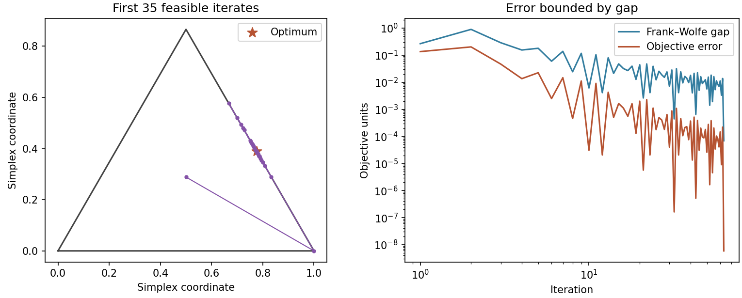
The reference projection in the example computes the exact quadratic optimum for comparison. The conditional-gradient method itself never calls that projection. The distinction lets you test its gap bound rather than inferring convergence only from a decreasing trace. Recompute the gap after the last update so it describes the point actually returned.
A compact feasible set and a smooth objective support the usual convergence analysis. An unbounded oracle or a nonsmooth objective changes the problem. Variant methods can address additional structure, but do not transfer the basic guarantee without checking their assumptions. The survey [5] explains alternatives and their geometric motivation.
Prove the oracle gap, including an inexact oracle
The conditional-gradient gap is the improvement allowed by the best linearized feasible direction. Convexity gives . Since the exact oracle minimizes that linear score over ,
Here is the current feasible point, an optimizer, and the exact linear-oracle solution. The first inequality uses objective convexity; the second uses the oracle’s comparison with . These are the two ingredients that turn a computable directional quantity into a global error bound [5].
If a feasible approximate oracle returns satisfying , with known , then the valid bound is the computed gap plus . Here is the oracle’s linear-objective error allowance. Feasibility of the update remains intact because , even when the gap needs correction.
For a simplex gradient , the exact oracle chooses its second vertex, whose score is . Choosing the first vertex gives score , requiring allowance . At , the exact gap is , but this approximate-oracle gap is . Adding three recovers . A negative uncorrected gap here indicates a poor oracle, not an objective error below zero.
7. Choose a method by structure, accuracy and information
There is no universally best update equation. The modeling decisions determine what information is available and which operations are inexpensive. Compare those operations before comparing a method’s name or its iteration count.
For a modest smooth problem with exploitable curvature, Newton or an interior-point method may reach a precise solution through relatively few expensive steps. For a huge sparse model, factorization memory can dominate; first-order methods may use cheaper matrix–vector products. For a simple nonsmooth penalty, a proximal operation can be exact and cheap. For a complicated set with an easy linear oracle, conditional gradients may avoid a costly projection.
Distributed optimization introduces communication as another expensive operation. Local objectives may be separable while consensus constraints connect variables. ADMM can expose local subproblems, but convergence time must include communication rounds and local solve cost. A mathematically distributed formulation does not imply the implementation runs in parallel; the denoising example is entirely serial.
Primal–dual hybrid-gradient methods handle saddle-point formulations using primal and dual updates [4]. Their step sizes depend on operator norms and the structure of the split terms. Practical linear-programming systems such as PDLP [6] add preprocessing and adaptive techniques around that structure. A short theoretical recurrence and a production solver are different levels of description.
Requested precision can reverse a comparison. A method that rapidly produces a useful approximate solution may take much longer to achieve a very small certificate gap. Another method may spend substantial setup time but converge efficiently to high precision. Plot time to several stated tolerances, and report original-unit feasibility alongside the gap. This makes the trade-off reviewable.
Memory and repeated solves matter too. A parameter sweep can reuse data structures, factorization or a previous solution when supported. A different sparsity pattern may prevent that reuse. Include preprocessing and setup in the first-solve measurement, then separately report warm repeated solves. Do not compare one method’s warm run with another’s cold run silently.
Consensus: local solves and a shared average
Distributed ADMM makes the communication mechanism explicit. Suppose participants share a vector decision but each has a local convex cost . Introduce local copies and shared variable , and solve with for every .
In scaled form, one consensus iteration is
Here is participant ‘s scaled multiplier, the penalty, and the iteration index. The first row consists of independent local solves. The second row minimizes the sum of quadratic consensus terms in , whose derivative sets to their average. The third row accumulates disagreement [3].
For scalar costs , the local solve is , where is a local target. Two participants with targets zero and four must agree at the globally optimal value two. Their individually optimal values zero and four violate consensus; averaging and multiplier updates coordinate the compromise.
Communication is therefore part of the algorithm: the shared update needs each local quantity, while each local solve needs the latest shared value. A parallel implementation must measure message cost and synchronization as well as local arithmetic. Additional shared constraints change the subproblem, often from a simple average to a constrained proximal operation.
8. A complete convex-optimization capstone
A capstone should make the formulation and evidence reproducible. Choose a synthetic signal estimator, geometric placement task or resource model. Write variables and units, a convexity argument, domains and a feasible-set interpretation before running the solver. State any relaxation and how its output becomes an implementable decision.
Build one small instance with an analytic answer or an independently computed certificate. Use it to check signs, shapes, scaling and stopping rules. Then vary one property at a time: noise strength, regularization, condition number, sparsity, problem size or tolerance. Keep the data seed fixed when comparing algorithms on the same instance.
Record objective values and residuals at the point actually returned. For splitting, track the coupling residual and the dual residual. For a conditional-gradient solve, report the current gap and oracle accuracy. For a barrier solve, distinguish the outer target from the computed certificate. For a relaxation, keep the lower bound and feasible rounded upper bound separate.
Assess the application outcome alongside numerical convergence. A denoiser may accurately minimize a penalty that removes a real event. A placement solver may obey every modeled rule while omitting a doorway requirement. A resource optimizer may be sensitive to an uncertain demand estimate. These are model-validation findings, not reasons to blur the meaning of a mathematical certificate.
For learned pipelines, split data before selecting regularization or fitting any preprocessing. Repeat solves on a validation set, choose the rule, then report the held-out outcome. The ML/DL evaluation chapter provides the broader learning protocol. Numerical convergence and predictive evaluation answer different questions and should appear in separate columns of the result table.
Modern view
The modern reading map combines surveys that organize algorithms with recent work that changes practical modeling or solving. The sources below were checked through October 4, 2026; unpublished manuscripts are identified explicitly.
Parikh and Boyd [2] organize proximal methods around the operation of solving a small convex subproblem. Boyd et al. [3] organize ADMM around separability, coupling and distributed statistical applications. Our teaching synthesis is to examine which subproblems become easy after a split and which new residuals must then be controlled. Splitting is valuable when it reduces total work, not simply because an objective has several terms.
Condat et al. [4] unify proximal splitting through primal–dual product spaces and monotone inclusions, revisiting parameter ranges and algorithmic variants. The reading connects apparently different recurrences through their operators and metrics. Use it to identify a method’s actual assumptions, especially when a smooth quadratic term permits choices different from a generic smooth function. The unified perspective prevents arbitrary parameter combinations from being treated as guaranteed methods.
Pokutta’s 2024 introduction [5] maps conditional gradients through linear oracles and feasible combinations. It helps compare projection-based methods with oracle-based alternatives and explains why feasible-set geometry affects behavior. The practical takeaway is to price the oracle and the representation, then use a valid gap. A cheap oracle can still require many iterations to obtain the precision an application needs.
The 2024 multi-robot survey by Shorinwa et al. [7] distinguishes distributed first-order, sequential convex-programming and ADMM approaches. It places communication, coordination and physical constraints alongside mathematical updates. Some robotics formulations are nonconvex or solved by successive convex subproblems, so convergence of a convex subproblem does not certify a global solution of the original trajectory or coordination task.
Applegate et al.’s PDLP manuscript [6], posted in 2025 and revised in 2026, provides recent evidence for practical large-scale first-order linear programming. Schaller, Bemporad and Boyd’s 2025 manuscript [8] instead fits parameterized convex functions compatible with disciplined programming. The former concerns a solver pipeline; the latter concerns learned functions that retain convexity in decision variables. Both are manuscripts, and neither makes arbitrary neural-network training convex.
| Question | Useful family or reading | Evidence to collect |
|---|---|---|
| Is a constraint projection cheap? | projected/proximal methods [2] | projection cost and optimality residual |
| Can terms be split into easy pieces? | ADMM and primal–dual splitting [3,4] | local solve cost and coupling residuals |
| Is linear minimization easier than projection? | conditional gradients [5] | oracle cost, feasible iterate and gap |
| Does communication dominate? | distributed-method taxonomy [7] | rounds, messages, local work and physical feasibility |
| Is the linear model too large for factorization? | practical first-order LP [6] | memory, accuracy and original-unit residuals |
| Can learned functions preserve decision-variable convexity? | parametric convex modeling [8] | structural restrictions and held-out model adequacy |
Our synthesis is that modeling and computation increasingly meet in reusable structured components: convex subproblems, inexpensive proximal maps, learned convex functions and hardware-aware solver operations. Their value still depends on an explicit formulation, valid assumptions and measured end-to-end behavior. A solver benchmark does not establish generalization; a prediction benchmark does not establish feasibility.
Open problems include automatic structure detection, robust certificates under poor scaling, communication-efficient solves, differentiability when active constraints change and reliable integration of learned predictions with exact constraints. A useful research question isolates one issue and preserves an independently checkable outcome. For example: “Does this warm start reduce total solve time while preserving the same certificate tolerance?”
The track now supplies a complete path: convex sets and functions, problem formulation, duality, estimation, numerical methods, constrained solvers and structured applications. Continue by choosing one textbook exercise family and building a small original experiment around its assumptions. The central habit is to state what is optimized, why the model is convex, what the algorithm computes and what evidence justifies accepting the result.
Key takeaways
- Geometric modeling includes projection, separation, centers, ellipsoids and structured placement.
- Unknown discrete choices and disjunctions can make the original application nonconvex.
- Relaxed lower bounds and feasible implementable solutions have different roles.
- Proximal operations handle simple nonsmooth penalties and constraints directly.
- ADMM splits coupling into tractable operations and requires primal and dual residual checks.
- Conditional gradients maintain feasibility through a linear oracle and supply a gap under stated assumptions.
- Compare original-unit accuracy, setup, memory, repeated solves and application outcomes.
Exercises
- Geometric center. Derive the largest inscribed ball for an axis-aligned rectangle. Explain why its center may be nonunique when one side is longer than the other.
Hint
The shorter side limits the radius. The center can move along the longer dimension while maintaining enough boundary clearance.
- Floorplanning model. Write convex nonoverlap constraints for two rectangles after choosing which one is left of the other. Explain what changes if the ordering is unknown.
Hint
A fixed order gives an affine separation inequality. Unknown order requires an either-or choice, which is a disjunction rather than one convex halfspace.
- Regularization sweep. Run the denoising example with five regularization strengths. Compare objective value, synthetic reconstruction error and the number of nearly zero adjacent differences.
Hint
Objectives with different regularization strengths are different functions, so their raw values are not a fair convergence comparison. Keep model quality and solve accuracy separate.
- Penalty update. Change the ADMM penalty halfway through the experiment. Update the factorization and scaled dual variable consistently, then compare residual traces with the fixed-penalty version.
Hint
The unscaled multiplier is the penalty times the scaled dual variable. Preserve that product when changing the penalty.
- Inexact oracle. Replace the simplex linear oracle with a deliberately suboptimal vertex. Identify how its objective error changes the certificate bound and whether the iterate remains feasible.
Hint
Feasibility follows from convex combinations of vertices. The gap based on an inexact oracle needs an additive bound on the oracle’s linear-objective error.
- Capstone report. Compare two appropriate algorithms on one synthetic convex application. Include the formulation, convexity proof, stopping policy, original-unit residuals, timing, memory and one model failure.
Hint
Use identical data and acceptance tolerances. Separate setup from repeated-solve costs, and report an unresolved numerical run rather than counting it as a successful solve.
References
- S. Boyd and L. Vandenberghe, Convex Optimization, Cambridge University Press, 2004, Chapter 8, with Chapters 4 and 6 for modeling and approximation. Book
- N. Parikh and S. Boyd, “Proximal Algorithms,” Foundations and Trends in Optimization, 2014. Survey
- S. Boyd, N. Parikh, E. Chu, B. Peleato and J. Eckstein, “Distributed Optimization and Statistical Learning via the Alternating Direction Method of Multipliers,” Foundations and Trends in Machine Learning, 2011. Review
- L. Condat, D. Kitahara, A. Contreras and A. Hirabayashi, “Proximal Splitting Algorithms for Convex Optimization: A Tour of Recent Advances, with New Twists,” SIAM Review, 2023. Author manuscript
- S. Pokutta, “The Frank-Wolfe Algorithm: A Short Introduction,” Jahresbericht der Deutschen Mathematiker-Vereinigung, 2024. Survey
- D. Applegate, M. Díaz, O. Hinder, H. Lu, M. Lubin, B. O’Donoghue and W. Schudy, “PDLP: A Practical First-Order Method for Large-Scale Linear Programming,” arXiv preprint, 2025, revised 2026. Paper
- O. Shorinwa, T. Halsted, J. Yu and M. Schwager, “Distributed Optimization Methods for Multi-Robot Systems: Part 2—A Survey,” IEEE Robotics & Automation Magazine, 2024. Survey
- M. Schaller, A. Bemporad and S. Boyd, “Learning Parametric Convex Functions,” manuscript, June 2025. Author page
Check your understanding
This tutorial has 6 exercises. Can you solve them without opening the hints?
Go to the exercises ↑This is the last tutorial in Optimization. Back to the learning map →