OPT 04 · Duality, KKT Conditions and Certificates
Needs: OPT 03 · Linear, Quadratic, Conic and Geometric Programs
Navigate: this page and this track: Navigate: this page and this track
On this page
- What you’ll learn1 min
- The big picture1 min
- From constraints to the Lagrangian1 min
- Why the dual problem is concave1 min
- A complete one-dimensional derivation1 min
- Strong duality and constraint qualifications2 min
- KKT optimality conditions1 min
- Equality-constrained quadratics1 min
- Deriving an LP dual carefully1 min
- Sensitivity and the value of a constraint2 min
- Infeasibility certificates1 min
- Cones, saddle points and numerical gaps3 min
- Modern view1 min
- Key takeaways1 min
- Exercises1 min
- References
Optimization
Explore this chapter 1 interactive experiment
Change a candidate point and multiplier. A small gap is meaningful only with feasibility.
What you’ll learn
- Derive a lower bound on a constrained minimization problem from a Lagrangian.
- Distinguish dual feasibility, weak duality, strong duality and attainment.
- State the KKT conditions and identify when they certify global optimality.
- Interpret complementary slackness and sensitivity with the correct multiplier signs.
- Construct a simple infeasibility certificate and extend dual order to cones.
- Report residuals and gaps without claiming more than numerical evidence supports.
The big picture
Finding a good feasible answer gives an upper bound on the best possible cost. How do we know that a much better answer is not hidden elsewhere? A dual problem produces lower bounds. When an upper and lower bound meet, they certify the optimum.
Boyd and Vandenberghe’s Chapter 5 [1] connects this idea to geometry, supporting planes, multipliers and numerical algorithms. Duality is useful even when we already know how to solve the primal problem: it verifies an answer, describes the value of limited resources and reveals alternative computational structure.
The guarantee must respect signs and assumptions. A value computed from arbitrary multipliers may not be a lower bound. A small stationarity residual alone is not a complete certificate. Strong duality is not automatic for every convex formulation.
This chapter develops the derivations with explicit domains and uses small examples whose exact answers can be checked. The resulting reasoning extends to large problems, but the implementation details and tolerances remain part of the numerical assessment.
From constraints to the Lagrangian
Plain version. Attach a price to every inequality and equality. Then minimize the priced objective without explicitly enforcing those constraints.
Consider
is the decision vector, is the common domain retained during minimization, is the objective, are inequalities and are equalities.
The Lagrangian is
are inequality multipliers and equality multipliers. For the convention , require . Equality multipliers are unrestricted because equality residuals vanish at feasible points regardless of sign.
At a feasible point, the inequality contribution is nonpositive and the equality contribution zero. Thus for nonnegative .
Calling these multipliers “penalties” can be misleading. This Lagrangian is not simply a large positive cost added to violations during an unconstrained minimization. Its role is to create a lower-bound family, and the sign condition is selected for that purpose.
Define the dual function
is the Lagrange dual function; its input is the multiplier pair. It takes the infimum over every point in , not just feasible points.
For any feasible and nonnegative ,
The first inequality follows from taking an infimum. The second follows from primal feasibility and multiplier signs. Therefore is a lower bound on the primal optimal value.
If the infimum is negative infinity, the bound is valid but uninformative. Dual feasibility includes multipliers with an appropriate finite dual value when we want a useful certificate.
Why the dual problem is concave
Plain version. The lower bound changes with prices. We choose the prices giving the strongest bound, and that maximization has a concave objective.
For each fixed , is affine in the multipliers. The pointwise infimum of affine functions is concave. Therefore is concave even if the original problem is not convex.
The dual problem is
Let its optimal value be . Weak duality states , where is the primal optimal value. This result does not require convexity, only the lower-bound construction with the correct signs.
A concave maximization is a convex optimization problem in the usual sense. However, evaluating the dual function can itself be difficult if it requires a hard nonconvex minimization. “The dual is concave” does not automatically provide a practical oracle.
The dual also need not have the same dimension as the primal. There is one variable for each explicitly dualized constraint. Retaining some restrictions in rather than attaching multipliers changes the written dual representation, while the lower-bound logic remains consistent.
The concavity proof in three lines
The dual is concave because the bound at mixed prices is at least the same mixture of the individual bounds. Let collect the multipliers, and take two allowed choices and . Affinity of the Lagrangian in prices gives
Here is the retained primal domain and the dual function; consider finite dual values for this comparison. Each summand at a shared is at least its own infimum, which explains the middle inequality. Nothing in that step assumes the primal objective is convex [1].
This distinction matters computationally. For a nonconvex primal, merely finding a local minimum of does not evaluate its infimum. That local value can exceed and cease to be a valid lower bound. Dual concavity concerns the exact dual function, not any approximate routine called a dual evaluator.
A complete one-dimensional derivation
Plain version. A small example shows how prices, the unconstrained minimizer and the bound fit together.
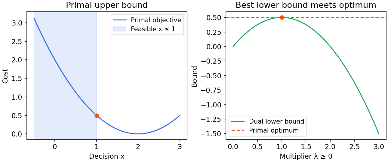
Minimize subject to . Here is scalar. The constrained optimizer is , with cost .
Using multiplier ,
The unconstrained Lagrangian minimizer satisfies , so . Substitution yields
depends on the selected multiplier and need not be primal feasible. The dual is a concave parabola, maximizing at with . Upper and lower bounds meet.
The optimum multiplier balances the objective’s desire to increase against the active upper-bound constraint. If is too small, the Lagrangian minimizer lies outside the allowed region. If it is too large, the bound becomes weaker despite the larger multiplier.
Code: verify the gap and all KKT components
This standalone calculation checks primal feasibility, multiplier sign, stationarity, complementary slackness and equality of the two values.
Code · Python · 14 lines
import numpy as np

x, multiplier = 1.0, 1.0
objective = 0.5 * (x - 2)**2
dual_value = multiplier - 0.5 * multiplier**2
constraint = x - 1
stationarity = x - 2 + multiplier
complementarity = multiplier * constraint
assert constraint <= 0 and multiplier >= 0
assert abs(stationarity) < 1e-12
assert abs(complementarity) < 1e-12
assert np.isclose(objective, dual_value)
print("primal value:", objective, "dual value:", dual_value)
print("stationarity:", stationarity, "complementarity:", complementarity)
Strong duality and constraint qualifications
Plain version. Weak duality always gives the ordering. Strong duality says the best lower bound is exact, which needs additional conditions.
Strong duality means . It is a statement about optimal values, not automatically about whether optimizers exist. A problem can have a value approached by a sequence without attaining it.
For a convex primal with affine equalities, a standard sufficient condition is Slater’s condition [1, Section 5.2]:
is the common function domain, its relative interior, and define the affine equality constraints. This says there is a point strictly satisfying inequalities while remaining in the appropriate interior and satisfying equalities.
Under these assumptions, strong duality holds. With a finite optimal value, the dual optimum is also attained. The primal attainment question can still require separate existence reasoning.
There are refined conditions for affine inequalities, so requiring all of them strictly can be stronger than necessary. A failure to find a Slater point does not by itself disprove strong duality. It means this sufficient argument has not been established.
Convexity alone is not enough in every formulation. Domains can be degenerate and constraint qualifications can fail. Rather than saying “convex problems always have zero gap,” state the condition being used or verify a valid matching certificate directly.
Domain restrictions are part of duality
If an objective contains a logarithm or inverse, its domain remains in the Lagrangian minimization. Treating it as a function on all real inputs silently changes the problem.
Alternatively, an extended-value function can encode a domain by assigning positive infinity outside it. This is mathematically convenient, but numerical code should not rely on accidental invalid floating-point values as a modeling convention.
In a conic formulation, domain and cone restrictions can be dualized or retained according to a consistent representation. The choice affects the dual expression and sign conventions. Derive the bound from the stated primal rather than copying a formula with incompatible signs.
Zero gap can coexist with no optimal multiplier
A failed constraint qualification does not force a positive duality gap, but it can remove multiplier attainment. Consider minimizing subject to , with scalar . The only feasible point is zero, so . There is no strictly feasible point.
The Lagrangian is . Minimizing over gives
Here prices the quadratic restriction and is its dual bound. For positive , the minimizing point is . As increases without bound, approaches zero. Thus , yet no finite multiplier attains the dual optimum.
At the primal solution, stationarity would require , which becomes . No KKT multiplier exists for this representation. Replacing the equivalent restriction by the equality gives a multiplier . The feasible decision is unchanged, but the regularity and multiplier description improve. This is why OPT 01’s hidden equalities and OPT 07’s initialization deserve attention [1].
KKT optimality conditions
Plain version. KKT combines allowed primal choices, allowed prices, balanced forces and the rule that slack constraints carry no positive price.
For differentiable convex and affine equality , the conditions are
is a primal candidate, are inequality multipliers, are equality multipliers, and the final row is stationarity of the Lagrangian. These are the Karush–Kuhn–Tucker conditions.
For this convex differentiable problem, satisfying all conditions is sufficient for primal and dual optimality. Nonnegative multipliers make the Lagrangian convex in ; stationarity makes its global minimizer; feasibility and complementary slackness make the Lagrangian value equal the objective.
Under a suitable constraint qualification such as Slater’s condition, optimal points also admit multipliers satisfying KKT. This supplies necessity as well as sufficiency. Keep the two logical directions distinct.
For nonconvex problems, a stationary Lagrangian can be a local maximum or saddle in . KKT may be necessary under regularity but does not generally certify a global optimum. A concave quadratic at its interior stationary point is a simple counterexample.
Complementary slackness is one-way information
If , complementary slackness forces . If , the constraint is active: .
An active constraint can nevertheless have zero multiplier. Degeneracy or redundant constraints can make prices nonunique. Therefore “active” and “positive price” are not interchangeable labels.
At a smooth constrained optimum, the negative objective gradient lies in the combination of active constraint normals and equality normals with appropriate signs. This gives a geometric explanation of stationarity: feasible descent directions cannot reduce the objective.
Numerical near-activity is tolerance-dependent. A constraint with a tiny slack and tiny multiplier may be difficult to classify discretely. Report actual values where the distinction matters instead of forcing a confident active/inactive label.
Equality-constrained quadratics
Plain version. For a quadratic objective and linear equalities, the KKT equations form one linear system. This reveals the algebra used by later constrained algorithms.
For objective under ,
is symmetric positive semidefinite, is the objective coefficient vector, the equality matrix, its target, and the equality multiplier.
The block matrix is generally indefinite even though the optimization problem is convex. A solver requiring a positive-definite matrix cannot be used blindly on this full KKT system.
If is positive definite and has independent rows, the system is nonsingular. More general cases require considering curvature on the equality nullspace and redundant constraints. A pseudoinverse may produce one solution but should not hide the underlying rank issue.
The equality multiplier balances the gradient in directions normal to the feasible affine set. Its sign is unconstrained. Removing a constraint changes both the feasible set and the meaning of its multiplier.
Deriving an LP dual carefully
Plain version. A dual formula is not universal notation. Its signs follow from the exact primal convention.
Take the LP subject to . Retain nonnegativity in the domain. The Lagrangian is .
Taking the infimum over nonnegative is finite exactly when . If any coefficient is negative, that coordinate can grow without bound and send the infimum to negative infinity.
Set . The dual becomes
is an unrestricted equality-price vector. For any feasible pair,
The gap is the inner product of nonnegative primal coordinates and nonnegative dual slack. This is weak duality in a particularly transparent form.
Using a primal maximization or reversed inequalities changes the dual signs. Rather than memorizing separate tables, deriving the Lagrangian and checking the bound can prevent mistakes.
A fitting dual built from the norm conjugate
Duality can turn a parameter penalty into a residual restriction. Consider sparse linear fitting with objective , where are fixed and . Introduce residual variable and an unrestricted equality multiplier :
Here is the parameter vector and has one coordinate per observation. Minimizing in gives and value for the residual terms. Minimizing in is finite exactly when , by the norm-conjugate calculation in OPT 02. The dual is therefore
Here is the dual variable; the norm restriction is dual feasibility. At an optimum it coincides with the fitted residual, while its correlations with the design columns must stay within the penalty threshold. This links the lower-bound construction to the geometry of sparse fitting [1, Chapters 5–6].
For synthetic , and , the primal solution is and dual candidate . Both are feasible for their respective problems and both objective values equal . Matching values certify the fit; observing zero coordinates alone would not.
Sensitivity and the value of a constraint
Plain version. A multiplier measures how the best cost responds to changing a constraint, under specified regularity. Its units depend on the constraint’s units.
Perturb inequalities to and equalities to . Let the best cost be . If strong duality holds at zero perturbation and optimal multipliers exist,
and are right-side perturbations; are optimal unperturbed multipliers. Positive relaxes an inequality under the chosen convention.
The inequality gives a global affine lower bound on the perturbed value. If the value function is differentiable at the original problem, its derivatives are and .
Without differentiability, multipliers can describe supporting slopes rather than one unique derivative. A large multiplier signals sensitivity in that local modeling direction, not a universal physical importance score.
A scalar example with a changing bound
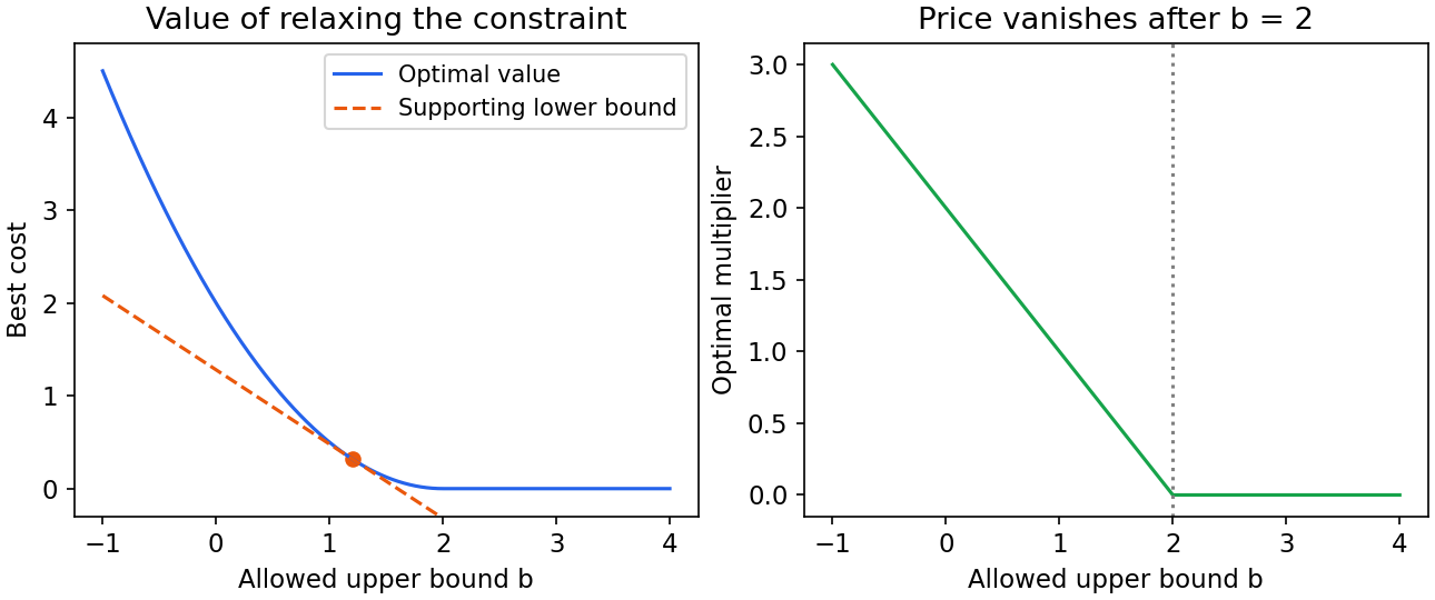
Minimize under . The best point is and the value is
is the allowed upper bound. Where differentiable, . Once the bound exceeds the unconstrained target, relaxing it further does not help and the multiplier is zero.
Scaling the constraint changes the multiplier reciprocally. Multiplying by a positive factor preserves feasible points but rescales its associated price. Compare sensitivity only after accounting for units and normalization.
Code: a finite-difference sensitivity check
Code · Python · 12 lines
import numpy as np

value = lambda b: 0.5 * max(2 - b, 0)**2
b, eps = 1.2, 1e-5
multiplier = max(2 - b, 0)
derivative = (value(b + eps) - value(b - eps)) / (2 * eps)
assert np.isclose(derivative, -multiplier, atol=1e-8)
test_bounds = np.linspace(-1, 4, 50)
lower_bound = value(b) - multiplier * (test_bounds - b)
assert np.all([value(t) for t in test_bounds] >= lower_bound - 1e-12)
print("finite-difference derivative:", derivative)
print("negative multiplier:", -multiplier)
Deriving sensitivity from the same lower bound
The sensitivity inequality needs no new principle. Use the original optimal multipliers on the perturbed Lagrangian. For any point feasible under and ,
Here are the perturbation vectors and the starred multipliers are optimal for the unperturbed problem. Taking the infimum over perturbed feasible points and using strong duality at the original problem produces the previously stated value-function bound. The minus sign follows from subtracting the perturbed right-hand sides inside the Lagrangian.
For the scalar bound example at , the value is and . Increasing the bound by with gives actual value . Its decrease is , while the multiplier predicts first-order decrease . The lower-bound prediction stays below the actual value, with difference .
If the restriction is instead written , its multiplier is . The derivative of this restriction with respect to is , so its product with the multiplier still predicts slope . Prices depend on representation; the predicted change in the original cost is consistent [1, Section 5.6].
Infeasibility certificates
Plain version. A valid weighted combination of constraints can prove that no choice satisfies them. That is stronger evidence than an algorithm failing to find a point.
For inequalities , suppose a vector satisfies
define the inequality system and is a nonnegative certificate vector. If a feasible existed, multiplying and summing would give , a contradiction.
This is the geometry behind a theorem of alternatives such as the forms discussed in [1, Section 5.8]. It distinguishes a mathematical certificate from an unsuccessful search.
In floating point, the equalities and strict sign must be assessed relative to scale. A nearly zero transpose residual and a tiny negative certificate value may be inconclusive under accumulated errors. Numerical certification requires a suitable tolerance analysis.
Code: incompatible scalar inequalities
The constraints are and . Their nonnegative sum proves impossibility.
Code · Python · 10 lines
import numpy as np

G = np.array([[1.], [-1.]])
h = np.array([0., -1.])
certificate = np.array([1., 1.])
assert np.all(certificate >= 0)
assert np.allclose(G.T @ certificate, 0)
assert h @ certificate < 0
print("transpose residual:", G.T @ certificate)
print("certificate contradiction:", h @ certificate)
Cones, saddle points and numerical gaps
Plain version. The lower-bound argument extends to cone inequalities by choosing prices from the matching dual cone. A primal–dual solution can also be viewed as a saddle point.
For a cone , its dual cone is
ranges over the original cone and is a price vector. When a constraint is expressed as belonging to , choose signs so the dual-cone inner product supplies the intended lower bound. Orthants, second-order cones and positive-semidefinite cones have familiar self-dual structures under their usual inner products.
For matrix variables, the inner product is trace: for symmetric matrices. Complementary slackness is then a trace condition, not entrywise multiplication.
Under the appropriate primal–dual assumptions, a saddle point satisfies
and are optimal primal and dual points; ranges over the domain and . The first side maximizes prices at the feasible point; the second minimizes decisions at the optimal prices.
In practice, an objective difference is a certified gap only when both points are appropriately feasible and the dual value is correctly evaluated. Approximate feasibility can require corrected bounds. A relative gap should use a documented denominator that remains meaningful near zero or with negative objective values.
A complete LP certificate and an invalid near-solution
Consider minimizing subject to and . The primal point has cost one. In the LP dual convention derived above, the scalar dual variable is feasible because , and its value is one. These matching bounds prove optimality without enumerating every feasible point.
The dual slack is . Its inner product with the primal point is zero, making complementary slackness explicit. The second coordinate is expensive relative to the equality price and receives zero allocation. This interpretation follows from the coefficients and the stated equality; it is not a general feature-importance conclusion.
Now take the approximate point . It satisfies the equality exactly and has an apparently better objective, 0.98. It violates nonnegativity. Comparing that objective with the dual value produces a negative difference, but does not refute weak duality: the candidate is outside the feasible set.
A routine that displays only equality residual and objective could therefore report a misleading result. Check every bound and cone restriction, including those encoded through a solver’s variable-bound argument rather than an explicit matrix row.
Clipping the negative coordinate gives , which then violates the equality. A subsequent normalization gives in this particular example. Neither clipping nor normalization is a universally valid repair procedure for coupled constraints.
Approximate residuals need corrected reasoning
For an approximately feasible LP pair, the algebraic objective difference is
are candidate primal and dual vectors, the dual slack and the primal equality residual. The identity is exact algebra; a nonnegative certified gap additionally needs the required feasibility properties.
If and but , the residual term can have either sign. A small residual multiplied by a large price can matter. This is why an absolute equality tolerance by itself is not a universal objective-accuracy guarantee.
If dual slack is only bounded below by componentwise and , then . Here measures the worst negative slack. Large primal magnitude can amplify a tiny dual violation.
This inequality does not turn the approximate dual objective into a lower bound for every feasible primal point unless a valid bound on those points is also available. An unbounded feasible set makes that correction especially delicate. Avoid describing an arbitrary approximate multiplier as an exact global certificate.
Report primal residuals, negative-slack magnitudes, multiplier norms and objective differences together. If a rigorous certificate is required, use a valid repair, verified error bound or higher-precision check appropriate to the problem structure.
Modern view
Plain version. Modern large-scale methods use primal–dual structure directly, while applications increasingly differentiate through constrained solutions. Both rely on the same certificate and regularity ideas.
Applegate and colleagues’ PDLP report [2], first posted in 2025 and revised in 2026, develops large-scale LP computation with practical primal–dual steps and feasibility polishing. Its relevance here is that a useful system monitors feasibility as well as cost improvement; a low objective error with unusable constraint violations is a different outcome.
Pokutta’s 2024 survey [3] explains primal and dual convergence for Frank–Wolfe methods. A linear minimization over the feasible set gives a first-order gap from the supporting-plane inequality. This is related to a lower-bound certificate, while its assumptions and computation differ from a generic Lagrange multiplier dual.
Agrawal and colleagues’ differentiable convex optimization layers [4] connect structured formulations with differentiation through solutions. The original paper is from 2019; it is included as a foundation for current optimization-layer work, not mislabeled as a new 2026 result. Differentiability and conditioning can fail near degeneracy or active-set changes, so a valid convex solution does not automatically imply a well-behaved gradient.
Current questions include obtaining reliable certificates at very large scale, interpreting uncertainty when constraints are learned, differentiating through nonunique solutions and balancing precision against application latency. Keep optimization accuracy, model validity and learning generalization as separate evaluations.
Key takeaways
- Feasible primal points provide upper bounds; feasible dual points provide lower bounds.
- Multiplier signs follow the exact inequality convention.
- The dual function is concave even when the primal is nonconvex.
- Strong duality needs suitable conditions or a directly verified matching certificate.
- KKT is sufficient for convex differentiable problems and needs regularity for necessity.
- Complementary slackness and sensitivity have precise one-way and sign rules.
- Numerical residuals and gaps must be interpreted with scale and feasibility.
Exercises
- Derive the dual of minimizing under , treating as fixed data.
Hint
Minimize the Lagrangian over the scalar variable before maximizing its multiplier.
- Give an active inequality with zero multiplier at an optimum.
Hint
A redundant bound at an unconstrained minimizer works.
- Derive the LP dual using nonnegative variables retained in the domain.
Hint
The linear coefficient must be nonnegative for a finite infimum.
- Explain why KKT stationarity at the origin does not certify minimizing on .
Hint
The origin is a maximum of the objective.
- Construct a nonnegative weighted contradiction proving a pair of scalar inequalities infeasible.
Hint
Add an upper bound below a required lower bound.
- Rescale an inequality by ten. Derive the corresponding multiplier rescaling and explain why primal sensitivity stays consistent.
Hint
Preserve the Lagrangian product.
References
- Stephen Boyd and Lieven Vandenberghe, Convex Optimization, Cambridge University Press, 2004. Reading: Chapter 5, including duality, KKT, perturbation, alternatives and generalized inequalities. Official book, free PDF.
- David Applegate, Mateo Díaz, Oliver Hinder, Haihao Lu, Miles Lubin, Brendan O’Donoghue and Warren Schudy, “PDLP: A Practical First-Order Method for Large-Scale Linear Programming,” arXiv preprint, 2025, revised 2026. Verified paper.
- Sebastian Pokutta, “The Frank-Wolfe Algorithm: A Short Introduction,” Jahresbericht der Deutschen Mathematiker-Vereinigung, 126, 2024. Open-access survey.
- Akshay Agrawal, Brandon Amos, Shane Barratt, Stephen Boyd, Steven Diamond and J. Zico Kolter, “Differentiable Convex Optimization Layers,” NeurIPS, 2019. Official publication page.
Check your understanding
This tutorial has 6 exercises. Can you solve them without opening the hints?
Go to the exercises ↑Next OPT 05 · Approximation, Statistical Estimation and Experiment Design · 19 min