OPT 06 · Gradient Descent, Newton Steps and Numerical Reliability
Needs: OPT 05 · Approximation, Statistical Estimation and Experiment Design
Navigate: this page and this track: Navigate: this page and this track
On this page
- What you’ll learn1 min
- The big picture1 min
- A direction and a distance1 min
- Gradient descent and its assumptions2 min
- Conditioning changes the path2 min
- Armijo backtracking1 min
- Steepest descent depends on a norm1 min
- Newton’s local quadratic model2 min
- Self-concordance and controlled curvature1 min
- A stable convex logistic solver2 min
- Implementation and stopping reports4 min
- Modern view1 min
- Key takeaways1 min
- Exercises1 min
- References
Optimization
Explore this chapter 1 interactive experiment
See why a step size that works on a round bowl can diverge on a narrow one.
What you’ll learn
- Separate a search direction from the step length chosen along it.
- Derive a safe gradient step under a Lipschitz-gradient assumption.
- Implement Armijo backtracking with domain and iteration safeguards.
- Explain conditioning, norm-dependent steepest descent and Newton curvature.
- Interpret a Newton decrement and the assumptions behind rapid local convergence.
- Verify derivatives, linear solves and stopping evidence in a CPU example.
The big picture
Convexity tells us which answers are globally optimal. An algorithm tells us how to move toward one using information that can be computed. Those are complementary questions: a convex problem can still be badly scaled, expensive or numerically delicate.
Boyd and Vandenberghe’s Chapter 9 [1] develops unconstrained descent methods, gradient descent, steepest descent, Newton’s method, self-concordance and implementation. This chapter follows that progression, keeping the cost of each step and the meaning of a stopping test visible.
The examples solve deterministic convex objectives. Their guarantees should not be silently transferred to a neural network’s nonconvex training objective, a noisy derivative or a nonsmooth penalty. Useful ideas can transfer, but the proof assumptions must be checked again.
We first use a quadratic with an exact solution, then implement a smooth regularized logistic objective from scratch. Both run on a CPU with locally generated data and no solver package beyond NumPy.
A direction and a distance
Plain version. A descent iteration chooses where to point, then how far to travel. Combining those choices too early hides why a step is safe.
Write an iteration as
is the current decision vector, a search direction and the step length. For a differentiable objective , a strict descent direction satisfies .
The inner product is the directional derivative at zero step. By differentiability, a sufficiently small positive step lowers the objective and remains in an open domain around the current point. A large step can still increase it or leave the domain.
The direction may depend on a gradient, a Hessian, a metric or other structure. The line search evaluates candidate distances. Counting only accepted iterations can hide many rejected objective evaluations.
If the gradient is zero for a differentiable convex objective on an open convex domain, the supporting-plane inequality certifies a global minimizer. With constraints, zero unconstrained gradient is generally not the correct optimality condition; the next chapter uses constrained systems.
Exact and inexact line searches
An exact line search minimizes over allowed positive distances. That auxiliary one-dimensional problem can be costly or unnecessary.
An inexact search accepts sufficient decrease rather than solving the line problem precisely. It should also preserve the objective’s domain. For a logarithmic term, testing a candidate with an invalid argument is a failed domain test, not evidence about its objective.
Floating-point evaluation adds another distinction: a mathematically decreasing step can become indistinguishable from the current value at machine precision. Repeatedly shrinking until a comparison happens to pass is not a robust termination rule.
Gradient descent and its assumptions
Plain version. Gradient descent points opposite the gradient. A curvature bound tells us how small a fixed step must be.
The update is
is the step size. Assume the gradient is Lipschitz with constant on the relevant region:
are points whose connecting segment stays in that region. measures how rapidly the gradient changes; it is not a regularization coefficient or a loss value.
The smoothness inequality is
is a trial displacement. Substituting gives
The step therefore supplies descent whenever the assumptions and domain requirement hold. For a twice-differentiable objective, an upper Hessian eigenvalue bound can establish such an [1, Section 9.3].
When only convexity and smoothness are assumed, objective convergence is typically sublinear under the standard fixed-step analysis. Strong convexity adds a positive lower curvature bound and permits linear geometric convergence. Those words describe mathematical rates, not a promise that every implementation will be fast.
From one-step decrease to a convergence rate
Descent proves that the objective improves; a convergence rate quantifies how much work reaches a target error. For a convex differentiable function on with -Lipschitz gradient and an attained minimizer , use . The gradient supporting bound gives
Here is the current point, its next iterate and any minimizer. Expanding the squared distance after the update gives
All symbols retain their definitions above. Combine the first inequality with the earlier smoothness decrease bound to obtain
Summing this inequality over the first updates cancels the intermediate distances. Since objective values decrease, the last error is no larger than the average of those errors:
Here is the start and the point after updates. This is the concrete meaning of an objective rate: halving the guaranteed error generally requires twice as many iterations under this bound. It is a worst-case guarantee with these assumptions, not a claim about every observed trace [1].
Strong convexity and a stopping bound
If is -strongly convex, its supporting model includes . Minimizing that lower model yields
is the global minimum and a valid strong-convexity constant. A small gradient then gives an objective-gap bound with known units.
Without a verified positive , the same formula is not a certificate. A small gradient can coexist with a large distance to the solution on a very flat objective. A small parameter update can instead reflect an excessively small step.
Avoid stopping solely because several printed objective values look identical. Check a suitable residual, the model’s scale, the progress trend and an iteration or time limit.
Conditioning changes the path
Plain version. An elongated bowl has steep and flat directions. A step safe for the steep direction can make progress painfully slow along the flat one.
For a positive-definite quadratic,
is symmetric positive definite and fixed. The Hessian is . Its smallest and largest eigenvalues supply and .
The ratio describes this Euclidean curvature conditioning. A large ratio means a single scalar step size must accommodate very different directional scales. Coordinate units can therefore change the behavior of gradient descent substantially.
Standardizing variables or choosing a suitable metric can improve a path, but must transform constraints, coefficients and stopping norms consistently. A rescaled algorithm is not judged fairly by an untransformed parameter-distance threshold.
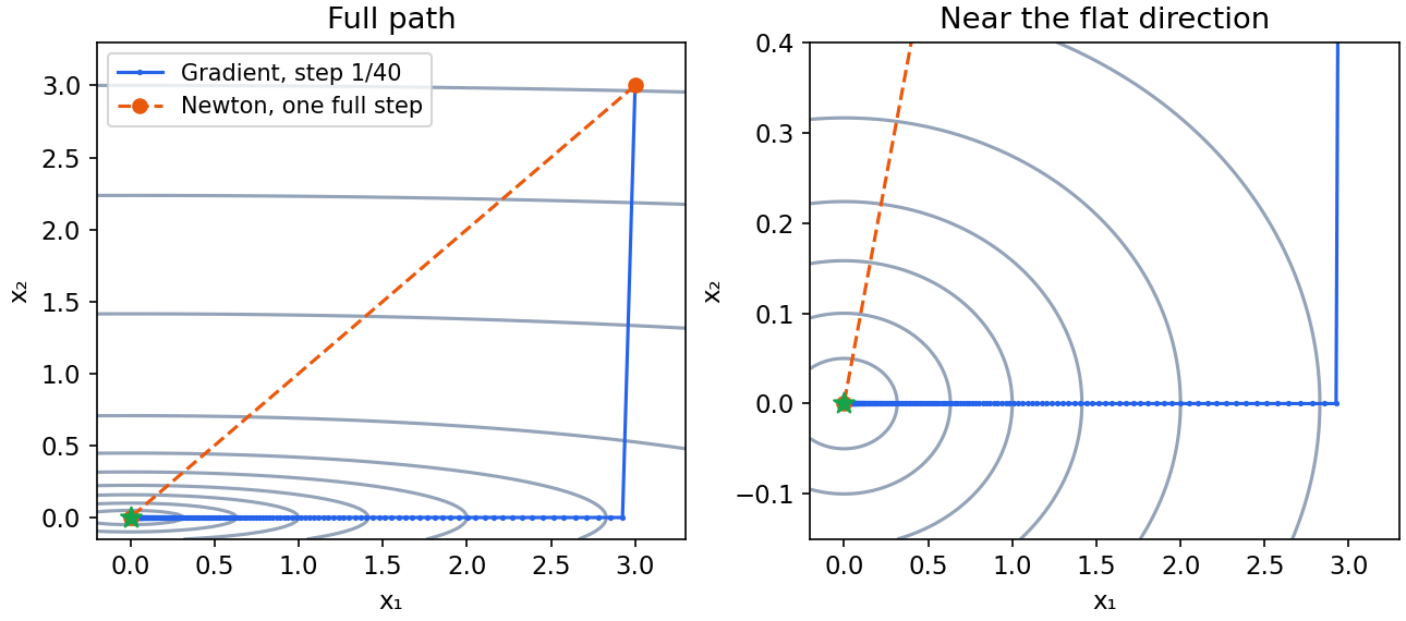
Code: compare a fixed gradient step and a Newton step
The objective is minimized at zero. We compare objective decrease and verify the Newton linear system rather than using an explicit matrix inverse.
Code · Python · 16 lines
import numpy as np

Q = np.diag([1., 40.])
x = np.array([3., 3.])
start = x.copy()
values = [0.5*x @ Q @ x]
for _ in range(200):
    x = x - (Q @ x)/40
    values.append(0.5*x @ Q @ x)
direction = np.linalg.solve(Q, -(Q @ start))
newton = start + direction
assert np.all(np.diff(values) <= 1e-12)
assert np.allclose(Q @ direction + Q @ start, 0)
assert np.linalg.norm(newton) < 1e-12
print("gradient objective after 200 steps:", round(values[-1], 8))
print("Newton objective after one step:", 0.5*newton @ Q @ newton)
A one-step Newton solution is special to an exact positive-definite quadratic with an accurate linear solve. On a general smooth function, curvature changes as we move and a full step may fail.
Read the quadratic path one eigenvector at a time
A quadratic makes the effect of the step size exact. Let be the error for a positive-definite quadratic with curvature . Gradient descent gives . In an eigenvector of with eigenvalue , the error coefficient is multiplied by .
Here is the fixed step, the identity, and the directional curvature. All coefficients contract precisely when , where is the largest eigenvalue. If , the steepest-direction error grows in magnitude even though the objective is convex.
For the chapter’s and , the steep coordinate disappears after one update, while the flat coordinate is multiplied by each time. Starting from therefore leaves first-coordinate error after updates. The gradual path is a consequence of directional curvature, not random numerical failure.
For a quadratic with smallest eigenvalue , choosing balances the magnitudes of the extreme contraction factors. Their worst value is . This choice improves the bound relative to a conservative step, but relies on known spectral endpoints and does not replace a line search for arbitrary nonquadratic functions [1].
Armijo backtracking
Plain version. Start with a candidate distance and shrink it until the decrease is large enough relative to the local slope.
The sufficient-decrease condition is
is a descent direction, the tested distance, and a fixed decrease fraction. Backtracking repeatedly multiplies by until the domain and decrease tests pass [1, Section 9.2].
For Newton methods, a usual choice keeps so full steps are accepted near a regular optimum under the standard local analysis. This is an assumption-aware choice, not a universal optimal parameter.
An implementation needs a maximum number of trials, a minimum meaningful step, finite-value checks and a clear failure report. Otherwise an invalid direction or an incorrect gradient can produce an endless shrinking loop.
What a rejected step tells us
A rejection can mean the initial distance was too ambitious, the curvature model was inaccurate far from the solution, the domain was crossed or the derivatives were wrong. It does not by itself identify which reason applies.
Check the directional derivative first. If it is nonnegative, ordinary descent backtracking lacks its intended justification. A modified direction may be needed, or the candidate may already meet an optimality test.
Repeated rejection near an optimum can come from floating-point cancellation. Compare objective and derivative scales before demanding an improvement below representable precision. Termination should explain which numerical condition was met.
Steepest descent depends on a norm
Plain version. “Steepest” requires a definition of one unit of movement. Different norms choose different directions.
The normalized steepest direction solves
is the direction, the chosen movement norm, and the current point. Under the Euclidean norm, a nonzero gradient gives direction .
For a positive-definite metric matrix , define . A corresponding unnormalized descent direction is
determines directional cost. The directional derivative is , strictly negative for a nonzero gradient.
Choosing resembles preconditioning: we account for known scale or curvature without necessarily forming the true Hessian. The usefulness depends on how cheaply the metric system can be solved and how well it represents the problem.
With a coordinate-based movement norm, steepest directions may select a coordinate or distribute movement differently. The book’s treatment [1, Section 9.4] explains why steepest descent is a family rather than one coordinate-independent procedure.
Newton’s local quadratic model
Plain version. Newton uses a quadratic approximation of the objective, then solves for the minimizer of that approximation.
At the current point, the model is
is the displacement, the gradient and the Hessian. When is positive definite, the model’s unique minimizing displacement solves
This is the Newton direction. Compute it through a linear solve or factorization, not by forming an inverse. Positive definiteness ensures a descent direction whenever .
Convexity gives a positive-semidefinite Hessian, which may be singular. A full Newton step is not automatically defined. A regularized Hessian, restricted subspace or another direction can be appropriate, but each changes the stated numerical procedure.
The Newton decrement
Define
is the Newton decrement and is assumed positive definite. The quadratic model predicts a decrease of at its minimizing step.
For an exact quadratic, that prediction equals the objective gap. For a general function, it is a local model quantity; a rigorous gap interpretation needs additional assumptions. Do not label the predicted decrease an unconditional global error certificate.
The direction and decrement transform coherently under an invertible affine change of coordinates when derivatives and solves are exact. This is one reason Newton behaves differently from Euclidean gradient descent. Floating-point conditioning and implementation still matter.
Local convergence is conditional
With suitable smoothness, a nonsingular positive-definite Hessian near the minimizer and an appropriate line search, Newton eventually accepts full steps and can converge quadratically [1, Section 9.5].
Quadratic convergence describes error shrinking approximately as the square of the previous error in a sufficiently small neighborhood. It does not imply that the first few steps from any initial point exhibit that behavior.
Errors in gradients, Hessians and linear solves can limit the rate. Far from the solution, safeguards may be essential. Near the solution, requesting a residual below derivative accuracy can waste work or trigger misleading failures.
Why Newton respects a change of coordinates
Newton adjusts direction using curvature, so changing variable units does not change its ideal physical step. Let with invertible matrix and fixed offset , and define . At corresponding points, the chain rule gives
Here are the gradient and positive-definite Hessian in coordinates, while tildes denote the same derivatives in coordinates. The transformed Newton equation is
Here is the displacement in new coordinates. Uniqueness of the solve gives , the original Newton displacement. Its predicted decrease is invariant too: .
Ordinary gradient descent instead maps its transformed step to , generally a different direction from . This connects coordinate scaling to the metric in steepest descent. Newton’s invariance assumes exact derivatives and solves; an ill-conditioned coordinate transformation can still harm a floating-point implementation [1, Section 9.5].
Self-concordance and controlled curvature
Plain version. Some convex functions control how quickly curvature changes through their own local curvature. This gives a special route to analyzing Newton steps.
For a standard self-concordant one-dimensional function,
is the scalar input and primes are derivatives, with nonnegative second derivative. In multiple dimensions, this condition is applied along lines in the domain [1, Section 9.6].
The logarithmic barrier on satisfies the scalar relation. This links unconstrained Newton analysis to the interior-point methods in the next chapter.
Self-concordance is more specific than ordinary smooth convexity. Its usefulness is that local norms can control changes without a single global Euclidean Hessian-Lipschitz constant. The theory includes precise decrement-based regions and complexity statements; those require the proper normalization and barrier assumptions.
A function containing logarithms is not automatically a valid barrier for every constraint representation. Its domain, boundary behavior and scaling must match the optimization problem. Distinguish a smooth likelihood term from a constraint barrier even if both contain a logarithm.
A stable convex logistic solver
Plain version. A complete implementation should evaluate the objective stably, verify its derivatives and stop using an optimality quantity.
For fixed rows and binary outcomes , use
is the parameter vector, the observation count and a regularization coefficient. Every coordinate is regularized in this example. The fixed-design logistic likelihood follows the convex-estimation reasoning in [1, Chapter 7].
Let . The derivatives are
stacks the rows, are observation vectors, and is the identity. The positive gives a valid global strong-convexity constant .
Use a stable softplus evaluation instead of taking the logarithm of a potentially overflowed exponential. The following bounded synthetic scores permit a direct sigmoid; for unrestricted extreme scores, use a numerically stable sigmoid implementation as well.
Derive the logistic curvature bounds
A stable objective is also easier to optimize when its curvature constants are known. For one score , the derivative of is , and its second derivative is . Thus subtracting the linear term gives gradient and Hessian .
Here is a fixed feature vector, the parameter vector, the observed label and the sigmoid probability. Average over observations and add the quadratic penalty to obtain the derivatives displayed above. Since ,
Here is the regularized average logistic objective, the feature matrix, the observation count, the penalty, and its largest singular value. The lower bound follows from full-coordinate regularization; the upper bound follows by testing for arbitrary direction .
Consequently and are valid global constants. They provide a safe gradient step and an objective-gap stopping bound for this specific model. If the intercept is left unpenalized, the same positive lower bound for every coordinate no longer follows. The mathematical formula, the penalty implementation and the stopping test must agree [1].
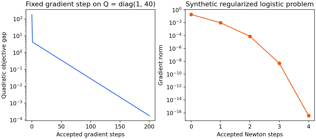
Code: Newton with derivative and stopping checks
This is an optimization demonstration, not a classification benchmark. It checks a directional derivative before solving and verifies the final gradient, decrease sequence and strong-convexity gap bound.
Code · Python · 54 lines
import numpy as np

rng = np.random.default_rng(16)
A = rng.normal(size=(160, 5))
truth = np.array([0.8, -0.5, 0.3, 0., 0.4])
prob = 1/(1+np.exp(-(A @ truth)))
y = (rng.random(len(A)) < prob).astype(float)
rho = 0.1

def evaluate(w):
    z = A @ w
    p = 1/(1+np.exp(-z))
    value = np.mean(np.logaddexp(0, z)-y*z) + rho*(w @ w)/2
    gradient = A.T @ (p-y)/len(y) + rho*w
    Hessian = (A.T * (p*(1-p))) @ A/len(y) + rho*np.eye(A.shape[1])
    return value, gradient, Hessian

w = np.zeros(A.shape[1])
direction = rng.normal(size=len(w))
eps = 1e-5
finite_difference = (evaluate(w+eps*direction)[0] -
                     evaluate(w-eps*direction)[0])/(2*eps)
assert np.isclose(finite_difference, evaluate(w)[1] @ direction,
                  atol=1e-8)
history = []
for iteration in range(30):
    value, g, H = evaluate(w)
    history.append(value)
    if np.linalg.norm(g) < 1e-9:
        break
    step_direction = np.linalg.solve(H, -g)
    slope = g @ step_direction
    assert slope < 0
    step = 1.0
    for trial in range(50):
        candidate = w + step*step_direction
        candidate_value = evaluate(candidate)[0]
        if np.isfinite(candidate_value) and candidate_value <= value+0.1*step*slope:
            w = candidate
            break
        step *= 0.5
    else:
        raise RuntimeError("backtracking did not accept a step")
else:
    raise RuntimeError("iteration limit reached")

value, g, H = evaluate(w)
assert np.linalg.norm(g) < 1e-9
assert np.all(np.diff(history) <= 1e-12)
assert np.linalg.eigvalsh(H).min() >= rho-1e-12
print("accepted Newton steps:", len(history)-1)
print("objective:", round(value, 8))
print("gradient norm:", np.linalg.norm(g))
print("objective-gap upper bound:", (g @ g)/(2*rho))
The derivative check tests one direction and one point; it cannot prove every derivative correct. Add checks at representative nonzero points when changing the model. Hessian symmetry, eigenvalue expectations and solve residuals provide additional independent evidence.
Implementation and stopping reports
Plain version. A solver result should describe why it stopped, what it verified and what computational work it performed.
Dense Newton stores a matrix whose size grows quadratically with the number of variables. Factorization can dominate the cost. Gradient methods often need only matrix-vector products, making many cheap iterations attractive for large problems.
Sparse matrices, low-rank terms and block structure can alter that comparison substantially. Exploit structure only after checking that the transformed system remains equivalent and that factorization fill-in is manageable [1, Section 9.7 and Appendix C].
A Hessian-vector product can support an iterative linear solve without explicitly storing the Hessian. Then the inner solve has its own residual and tolerance. A loosely solved Newton system need not reproduce the exact Newton direction or convergence rate.
Report objective values, a suitable gradient or stationarity residual, domain checks, iteration count and the stated stopping condition. Where timing matters, include derivative evaluations and line-search trials rather than only accepted steps.
Scaling the objective changes gradient magnitudes. A fixed absolute gradient tolerance is therefore not comparable across arbitrary loss normalization. Relative criteria need a documented scale and should remain meaningful near zero.
An iteration limit is a resource stop, not an optimality certificate. A line-search failure is an algorithmic diagnosis, not proof of nonexistence. Retain the final candidate and residual evidence so that the result can be assessed.
Exact quadratic line searches reveal a tradeoff
For the positive-definite quadratic above and a nonzero descent direction , the objective along the line is a scalar quadratic. Differentiating with respect to distance gives
is the current gradient, the positive-definite curvature and the minimizing line distance. This formula is an exact line search for this particular quadratic, not a general smooth objective.
For the negative gradient direction, the numerator becomes and the denominator is . The chosen distance accounts for curvature along that direction. It can outperform a conservative fixed step without correcting the underlying elongated geometry.
Successive directions can still zigzag. Exact minimization along one line does not imply that the line points directly toward the global minimizer. This makes the roles of direction and distance particularly clear: better distance selection cannot fully replace better directional geometry.
A Newton direction uses the whole quadratic curvature system, reaching the minimizer with distance one in exact arithmetic. A metric approximation may reduce the system cost while giving a less accurate route. The fair comparison includes how the metric is built and reused, not just the length of the visible path.
If a matrix factorization is reusable across many right-hand sides, its initial cost can be amortized. If the matrix changes at each iteration, that advantage may shrink. Likewise, an objective evaluation can be cheap in a tiny tutorial but expensive in an application with a simulation inside it. State the actual computational primitives before making a speed claim.
Derivative checks need a scale
A central finite difference divides the difference of two nearby objective values by twice the perturbation. Making the perturbation smaller reduces the ideal truncation error at first, but eventually amplifies floating-point cancellation.
Use several perturbation sizes and compare relative as well as absolute discrepancies. Scale the direction sensibly, choose test points away from a domain boundary, and inspect whether the result stabilizes over a useful interval. One failed tiny-step comparison may indicate numerical resolution rather than an incorrect derivative.
For a Hessian, compare a gradient difference with a Hessian-vector product. This tests a different layer of the implementation from checking objective differences alone. Also verify symmetry when the objective is twice continuously differentiable and the intended Hessian should be symmetric.
An automatic derivative system can remove much manual algebra but still differentiate the implemented expression rather than the intended model. Incorrect broadcasting, a misplaced reduction or an accidentally regularized intercept can yield a perfectly consistent derivative of the wrong objective.
Record these checks beside the formulation. The goal is to connect symbols to arrays, not merely to produce a green test. Once the implementation matches the model, numerical tolerances and algorithm assumptions can be assessed meaningfully.
A reproducible comparison also needs a starting point, objective normalization, stopping rule and numerical precision. Changing any of these can alter apparent convergence. Store the parameters and random seed with a synthetic experiment so that a later figure can be regenerated from the same stated problem.
For deterministic algorithms, small platform differences may still affect the final few digits or a marginal line-search comparison. Verify properties with justified tolerances instead of asserting one exact decimal trajectory. The examples here check descent, linear-system consistency and gradient evidence, which are the quantities tied to the formulation.
Modern view
Plain version. Modern convex algorithms trade curvature information, projections, proximal operations and communication costs. The right choice depends on structure and required accuracy.
Dvurechensky, Shtern and Staudigl’s first-order survey [2] provides a broad foundation, including non-Euclidean proximal methods, acceleration and projection-free approaches. It was published in 2021; it is a background map rather than a new 2026 result.
Condat and colleagues’ 2023 SIAM Review survey [3] unifies proximal splitting for high-dimensional nonsmooth convex problems through primal–dual product spaces and chosen metrics. It explains why adding an absolute-value penalty changes the appropriate primitive: an ordinary smooth Newton formula cannot simply differentiate through the kink.
Pokutta’s 2024 Frank–Wolfe survey [4] focuses on linear minimization over constrained sets and its convergence and certificate structure. It complements the gradient/Newton comparison by asking whether a projection or expensive system solve can be avoided.
Together these reviews give a practical taxonomy: smooth versus nonsmooth objectives, inexpensive versus expensive feasible-set operations, Euclidean versus structured geometry, and local curvature versus cheap first-order steps. Recent variants do not remove those modeling distinctions.
Current issues include adaptive methods with reliable certificates, precision limits in large linear systems, communication in distributed problems and differentiating through solver outputs. Match the algorithm to the model, the hardware and the requested error measure; compare total work at a comparable accuracy.
Key takeaways
- A descent direction and a step length are separate choices.
- Fixed gradient steps require a valid curvature and domain argument.
- Poor conditioning slows a scalar-step gradient method.
- Backtracking needs safeguards and correct derivative signs.
- Newton uses a linear solve and has conditional local convergence.
- A decrement is a model quantity unless its gap assumptions are established.
- Reliable reports include stopping evidence and the cost of rejected work.
Exercises
- Derive the smoothness decrease inequality for a step of size .
Hint
Substitute the negative scaled gradient into the upper quadratic model.
- Replace the quadratic eigenvalue 40 by 400. Predict and test how fixed-step gradient progress changes.
Hint
The flat-direction contraction depends on the eigenvalue ratio.
- Implement backtracking for on , checking the domain before every objective evaluation.
Hint
Reject nonpositive candidates immediately.
- Verify the logistic gradient in three random directions at a nonzero parameter vector.
Hint
Compare central differences and inner products using several finite-difference scales.
- Show why a singular positive-semidefinite Hessian does not always define a unique Newton direction.
Hint
Inspect the linear system’s nullspace and consistency.
- Rescale the logistic objective by one hundred. Determine which stopping quantity and tolerance changes preserve the original requested objective accuracy.
Hint
Transform the gradient, strong-convexity constant and desired gap together.
References
- Stephen Boyd and Lieven Vandenberghe, Convex Optimization, Cambridge University Press, 2004. Reading: Chapter 9, Sections 9.1–9.7; Appendix C for linear systems; Chapter 7 for the logistic likelihood connection. Official book, free PDF.
- Pavel Dvurechensky, Shimrit Shtern and Mathias Staudigl, “First-Order Methods for Convex Optimization,” EURO Journal on Computational Optimization, 9, 100015, 2021. Verified open manuscript, published article.
- Laurent Condat, Daichi Kitahara, Andrés Contreras and Akira Hirabayashi, “Proximal Splitting Algorithms for Convex Optimization: A Tour of Recent Advances, with New Twists,” SIAM Review, 65(2), 375–435, 2023. Published survey, open manuscript.
- Sebastian Pokutta, “The Frank-Wolfe Algorithm: A Short Introduction,” Jahresbericht der Deutschen Mathematiker-Vereinigung, 126, 2024. Open-access survey.
Check your understanding
This tutorial has 6 exercises. Can you solve them without opening the hints?
Go to the exercises ↑Next OPT 07 · Equality Constraints and Interior-Point Methods · 21 min