OPT 03 · Linear, Quadratic, Conic and Geometric Programs
Needs: OPT 02 · Convex Functions, Composition and Conjugates
Navigate: this page and this track: Navigate: this page and this track
On this page
- What you’ll learn1 min
- The big picture1 min
- The convex standard form1 min
- Linear programming2 min
- Quadratic programming and convex QCQPs2 min
- Second-order cone programming2 min
- Semidefinite programming2 min
- Geometric programming2 min
- Quasiconvex problems through feasibility2 min
- Multiobjective decisions and Pareto tradeoffs1 min
- Modeling and numerical checks1 min
- Modern view1 min
- Key takeaways1 min
- Exercises1 min
- References
Optimization
Explore this chapter 1 interactive experiment
Compare coordinate clipping with the exact solution of a coupled quadratic under nonnegative constraints.
What you’ll learn
- Identify linear, quadratic and convex quadratically constrained programs.
- Turn absolute values, maxima and norm constraints into exact formulations.
- Express second-order and semidefinite cone constraints with the right ordering.
- Transform a geometric program into a convex problem using positive variables and logarithms.
- Separate exact reformulation, convex relaxation and approximation.
- Explain scaling, feasibility checks and multiobjective tradeoffs before selecting a solver.
The big picture
A model can be convex while its written form hides that fact. A sum of absolute residuals looks nonsmooth but becomes a linear program with auxiliary variables. A norm bound becomes a cone constraint. A positive-variable design can become convex after a logarithmic change of variables.
Boyd and Vandenberghe’s Chapter 4 [1] organizes these problem families. Learning them serves two purposes: it supplies reusable modeling patterns and helps choose numerical methods that exploit structure. The class is determined by equations and domains, not by the label attached to an application.
The examples in this chapter use synthetic small problems. They show exact mathematical relationships and numerical checks, not benchmark results. The code uses the installed numerical libraries without introducing a separate modeling-system dependency.
The convex standard form
Plain version. Convexity requires the objective, inequalities and equalities to fit together. It is not enough for the objective alone to be convex.
The standard form is
is the decision vector; are convex functions on their relevant common domain; is a fixed matrix and a fixed equality target. The feasible set is convex because convex sublevel sets and affine equalities are intersected.
A concave function can appear on the other side: is convex-feasible when is concave, because is a convex inequality. Equality to a nonlinear convex function is generally not convex. For example, describes a sphere surface, while describes a convex ball.
Writing an equality as two inequalities does not fix this issue. One of the two directions reverses the curvature. If the physical problem truly requires the surface, replacing it by a ball is a relaxation and may change the answer.
Exact reformulation versus changing the problem
An exact reformulation preserves the achievable original decisions and objective after auxiliary variables are eliminated or a one-to-one transformation is reversed. A relaxation enlarges the allowed set. An approximation changes functions or constraints to nearby ones.
For an epigraph variable , minimizing with is exact because the optimizer can choose the smallest permitted . Merely imposing the inequality inside another model may not force equality if the remaining objective does not prefer smaller .
When a reformulation adds variables, prove both directions: every original feasible point can be extended to a reformulated point, and every reformulated point maps back to an original feasible decision with the correct objective relation. This small proof prevents many modeling errors.
Linear programming
Plain version. A linear program uses straight-line costs and rules. Its geometry is a polyhedron, which can have corners, faces and directions extending to infinity.
An inequality-and-equality linear program is
is the fixed objective coefficient vector; define inequality bounds; define equalities. Bounds on individual variables can be included separately or as rows of .
A linear objective is both convex and concave. The restrictions need not force a unique solution. When an objective is parallel to a feasible face, every point on that face can be optimal.
A standard nonnegative form writes . Introduce nonnegative slack variables to turn inequalities into equalities, and represent a free scalar as the difference of two nonnegative scalars if this form is needed.
These transformations are exact but can increase size and change numerical conditioning. A solver interface may accept bounds and inequalities directly, so there is no need to expand everything manually for its own sake.
Absolute residuals become linear constraints
To fit measurements using design matrix , consider
is a fixed design matrix, its coefficient vector and the measurement vector. Introduce one variable for each residual:
bounds residual magnitudes and is the all-ones vector. Each feasible is at least the absolute residual, and minimizing their sum tightens the bounds. Nonnegativity of follows from the paired inequalities but can be specified explicitly.
Minimax fitting instead introduces one scalar and minimizes it subject to . This controls the largest absolute residual rather than their sum. The modeling change expresses a different application preference.
Code: solve a small allocation LP
The SciPy interface is documented in [2]. This example checks success and feasibility independently, rather than printing the optimizer without checking its status.
Code · Python · 14 lines
import numpy as np
from scipy.optimize import linprog

c = np.array([-3.0, -2.0])
G = np.array([[1.0, 1.0], [2.0, 1.0]])
h = np.array([4.0, 5.0])
result = linprog(c, A_ub=G, b_ub=h, bounds=[(0, None), (0, None)])
assert result.success, result.message
x = result.x
assert np.all(G @ x <= h + 1e-8)
assert np.all(x >= -1e-8)
assert np.allclose(x, [1, 3], atol=1e-7)
print("allocation:", x, "objective:", c @ x)
print("slacks:", h - G @ x)
The negative objective coefficients encode maximizing a positive benefit through minimization. The problem is bounded because the capacity constraints restrict nonnegative choices. Removing a relevant bound can make the model unbounded; that is a modeling outcome, not a solver defect.
Quadratic programming and convex QCQPs
Plain version. A quadratic program replaces the linear cost with a curved bowl while keeping linear rules. Quadratic inequality constraints are also possible if their bowls face upward.
A convex quadratic program, QP, has objective
with affine constraints. is a symmetric positive-semidefinite curvature matrix, is a linear coefficient vector and a constant that does not change the optimizer.
Least squares is a QP: expanding gives and . A quadratic regularizer adds positive diagonal curvature. If the design matrix is rank deficient, the unregularized minimizer may not be unique.
A convex quadratically constrained quadratic program, QCQP, also has inequalities
is each constraint’s curvature matrix, a linear coefficient vector and its offset. Arbitrary quadratic constraints do not meet this condition. An indefinite quadratic constraint can be nonconvex even if the objective is strongly convex.
Numerical structure matters
An unconstrained positive-definite QP solves . A constrained QP may have an optimizer at a boundary, so solving the unconstrained system and clipping afterward is generally wrong.
Clipping is correct for projection onto a box in ordinary Euclidean distance. A general quadratic couples coordinates; adjusting one coordinate changes the best value of others. The correct constrained solution must respect that coupling.
The size and sparsity of matter. Forming explicitly can destroy useful sparsity or worsen conditioning. A model can be written as a quadratic while its implementation retains residual operators. The algorithms chapters explain factorization and matrix-vector-product choices.
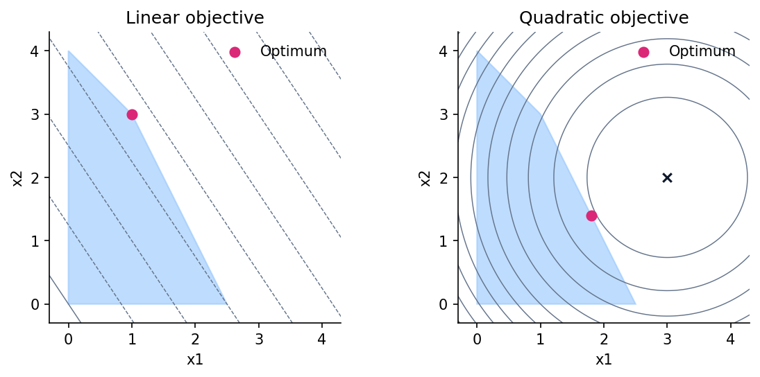
Worked counterexample: why clipping a QP is wrong
Coupled curvature can make changing one coordinate shift the best value of another. Consider the convex quadratic
Here is the variable, the unconstrained target and the positive-definite curvature matrix. Simply clipping produces with objective one. With , however, stationarity in the unrestricted second coordinate gives , hence .
The candidate has objective . Its gradient is , balanced by multiplier on . Feasibility, multiplier sign, stationarity and complementary slackness therefore verify the optimum using OPT 04’s conditions. Coordinate clipping ignores the off-diagonal entries of ; Euclidean box projection works because its quadratic separates by coordinate.
Second-order cone programming
Plain version. A second-order cone expresses a norm bound with a scalar on the right. It turns many curved constraints into a standard geometric form.
A common SOCP inequality is
define the vector inside the norm; define the affine scalar bound; and is the decision vector. The inequality automatically requires its right-hand side to be nonnegative.
Do not square both sides without retaining that sign condition. The squared inequality can allow a negative right-hand side and introduce extra points. The cone formulation carries the sign correctly.
A rotated second-order cone can encode quadratic-over-linear expressions. In a common convention, it requires and . The factor of two is a convention and must match the implementation.
Using expresses . Different scaling choices give the same mathematical set but can change numerical behavior.
Robust linear constraints
Suppose a constraint coefficient is uncertain: with . Requiring for every allowed gives
is the nominal coefficient vector, maps unit-ball uncertainty and is a fixed bound. The norm is the maximum of over the unit ball.
This is an exact robust counterpart for the specified uncertainty set. It does not guarantee protection against all real-world uncertainty; the set itself must be justified. A larger set can be more conservative, while an incorrect set can miss important disturbances.
The geometry of uncertainty determines the reformulation. Box uncertainty gives a one-norm term; ellipsoidal uncertainty gives a Euclidean norm after a transformation. These connections follow from support functions developed in the previous chapter [1].
Derive the robust counterpart rather than guessing a penalty
The robust norm term is the exact worst allowed disturbance. Expand the uncertain linear constraint:
Here is the decision, the nominal coefficient, the uncertainty map and an allowed disturbance. The last equality follows from the inner-product norm bound, with equality at when the denominator is nonzero. When it is zero, every disturbance contributes zero.
For the synthetic constraint with , the exact robust rule is . At its worst left side is , so it is robust feasible. The maximizing disturbance is proportional to . No tuning weight was invented: the added term follows from the stated uncertainty geometry [1].
Semidefinite programming
Plain version. A semidefinite program constrains a whole matrix to have nonnegative curvature in every vector direction. Checking entries individually is not enough.
A linear matrix inequality is
are fixed symmetric matrices; are scalar decision variables; and requires positive semidefiniteness. A linear objective with affine equalities and such constraints defines an SDP.
If all matrices are diagonal, positive semidefiniteness reduces to nonnegative diagonal entries, giving linear inequalities. General matrices include relationships between coordinates that cannot be captured by entrywise nonnegativity.
For example, the symmetric matrix
is positive semidefinite exactly when . Here is a scalar off-diagonal correlation. Negative is allowed despite entrywise negativity, while an excessively large positive makes the matrix indefinite.
Schur complements expose hidden forms
For positive-definite , a block matrix condition satisfies
is a positive-definite symmetric block, a vector and a scalar. The right side is the Schur complement. The positive-definiteness assumption is important; singular blocks need an additional range condition or a generalized argument.
This identity converts some matrix inverse expressions into affine matrix constraints when the block entries are affine in decision variables. Whether the result is convex depends on that affine structure, not just on displaying a block matrix.
Prove the Schur condition by completing a square
A block matrix is positive semidefinite when its quadratic form is nonnegative for every vector. For , a vector and scalar give
Here is the positive-definite block, a compatible vector, a scalar block, and arbitrary test coordinates. If , both terms are nonnegative. Conversely, choose and ; the first term vanishes, forcing that scalar inequality. This proves both directions of the equivalence [1].
It is also a modeling recipe. With fixed and affine vector , the upper bound becomes a matrix inequality affine in . If is a matrix decision variable, the same block representation can still be affine in its entries on the positive-definite domain. A nonlinear term can therefore have a convex epigraph even when its original inverse expression hides the structure.
The assumption enables the square completion and inverse. A singular cannot be handled by silently using the same formula; the vector’s range condition becomes part of the equivalence.
Code: distinguish matrix and entrywise order
This code checks a family with known eigenvalues and demonstrates a valid Schur-complement boundary.
Code · Python · 13 lines
import numpy as np

for r in [-0.8, 0.8, 1.2]:
    X = np.array([[1., r], [r, 1.]])
    eigenvalues = np.linalg.eigvalsh(X)
    print("r:", r, "eigenvalues:", eigenvalues)
    assert (eigenvalues.min() >= -1e-12) == (abs(r) <= 1)
P = np.array([[2., .3], [.3, 1.]])
q = np.array([.4, -.2])
t = q @ np.linalg.solve(P, q)
block = np.block([[P, q[:, None]], [q[None, :], np.array([[t]])]])
assert np.linalg.eigvalsh(block).min() >= -1e-12
print("Schur boundary t:", t)
This is a spectral check, not a full SDP solver. The course uses small direct calculations to explain the model without implying that a general nonlinear optimizer supplies all the certificates of a dedicated conic method.
Geometric programming
Plain version. Some positive-variable models look nonconvex in their original coordinates but become convex when multiplication turns into addition under logarithms.
In geometric programming, a monomial has the specialized form
is a positive coefficient and are arbitrary real exponents. This differs from the elementary algebra convention requiring nonnegative integer powers.
A posynomial is a sum of such monomials:
is the number of terms, their positive coefficients and their exponents. Negative coefficients are excluded.
A geometric program minimizes a posynomial, constrains posynomials to be at most one, and constrains monomials to equal one, with positive decision variables [1, Section 4.5]. Arbitrary sums, signs or equalities do not fit this class.
Derive the logarithmic transformation
Set , so . A monomial becomes ; its logarithm is affine. A posynomial’s logarithm becomes
holds the exponent vector of term . This is log-sum-exp of affine expressions, which is convex.
The logarithm is strictly increasing, so minimizing the original positive objective and minimizing its log produce the same optimizer after reversing the variable transformation. Posynomial inequalities become convex log-sum-exp inequalities, and monomial equalities become affine equalities.
The objective values are transformed, however: the log objective is not numerically the same as the original cost. Convert back when reporting the application quantity.
This is an exact change of variables on the positive domain. It is different from dropping negative terms or changing a non-monomial equality to an inequality. Those operations can create a different problem.
Code: a positive allocation in log coordinates
Minimize subject to and . Symmetry and the convex original objective establish the solution ; the transformed problem verifies the same answer numerically.
Code · Python · 17 lines
import numpy as np
from scipy.optimize import minimize
from scipy.special import logsumexp

objective = lambda z: logsumexp(-z)
constraint = {"type": "ineq",
              "fun": lambda z: np.log(4.) - logsumexp(z)}
result = minimize(objective, np.log([1., 1.]),
                  constraints=[constraint], method="SLSQP",
                  options={"ftol": 1e-12, "maxiter": 100})
assert result.success, result.message
x = np.exp(result.x)
assert x.sum() <= 4 + 1e-7
assert np.allclose(x, [2., 2.], atol=1e-5)
print("positive variables:", x)
print("original objective:", np.sum(1 / x))
print("transformed objective:", result.fun)
The numerical interface is documented in [3]. This small demonstration checks against an analytical solution. It does not make this general-purpose method a replacement for specialized geometric-programming solvers on all scales.
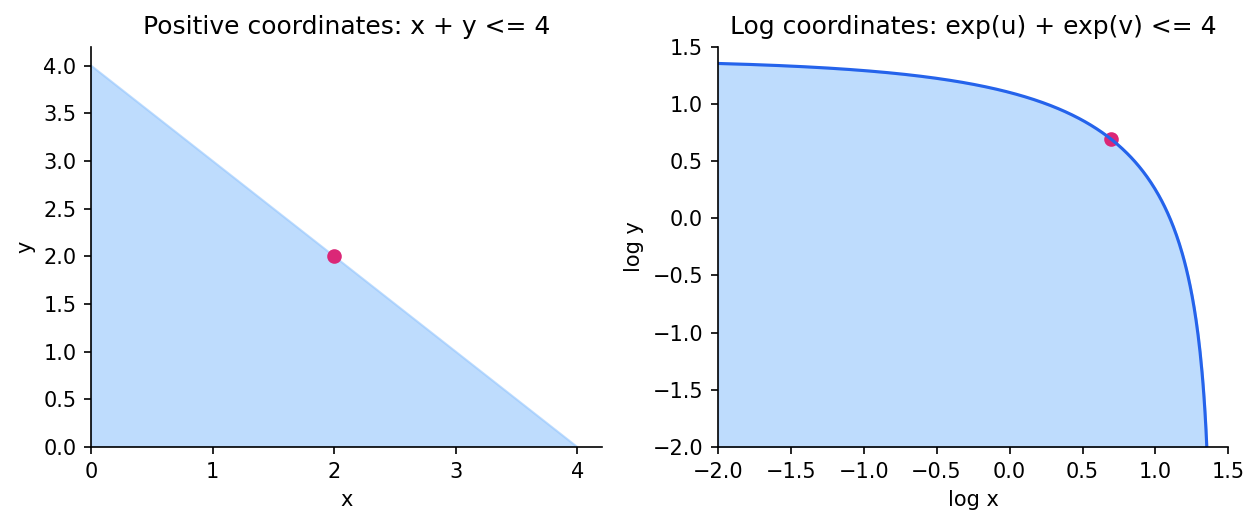
Worked design: an asymmetric positive allocation
A logarithmic transformation preserves the optimum, even when symmetry cannot supply the answer. Minimize under with . Since both terms decrease as their variables grow, the optimum uses the full budget.
Set . Differentiating the remaining scalar objective gives
Here are positive allocations and the star denotes an optimum. The second derivative is positive on , so the stationary point is the unique minimum. Its original cost is .
In logarithmic variables , , the objective becomes and the restriction becomes . Both are log-sum-exp expressions. The recovered solution is , with transformed cost . Reporting as the original cost would mix two coordinate systems. This example gives an analytical check for the entire transformation [1, Section 4.5].
Quasiconvex problems through feasibility
Plain version. Some useful objectives are not convex, but asking whether a proposed score is achievable gives a convex feasibility problem. A sequence of threshold questions can then find the best score.
Suppose the sets are convex and can be represented by convex constraints for each fixed threshold . Maintain a lower and upper bound on the optimal score. Test the midpoint threshold: if its feasible set is nonempty, lower the upper bound; if not, raise the lower bound.
Here the threshold is fixed while solving each feasibility problem. Treating it as another free variable can introduce nonconvex products or ratios. The convexity of every threshold problem does not imply joint convexity in the threshold and original decision.
For example, a positive-denominator affine ratio has convex sublevel sets on a convex domain where . At a fixed threshold , the score inequality becomes , an affine constraint in . Positivity of the denominator is essential to multiplying without reversing the inequality.
Numerical feasibility must be handled carefully. An approximate solver may be unable to distinguish an empty set from an extremely narrow feasible region near the optimal threshold. A failed iteration or uncertain status is not automatically an infeasibility certificate. Use an appropriate feasibility procedure and report the threshold interval and tolerances.
This approach is covered by the quasiconvex discussion in [1]. It broadens the course beyond convex objectives while keeping the role of convexity precise: the subproblems are convex, and bisection supplies the outer scalar search.
A modeling audit before solving
Take one original application requirement at a time and translate it to the chosen variables. Check whether its domain is enforced, whether a sign was changed correctly, and whether the formulation preserves its units. Then trace how auxiliary variables are eliminated.
Consider a worst-case norm constraint expressed through a scalar upper bound. If the auxiliary scalar is absent from the objective, it may remain unnecessarily loose. That can still be correct if only an upper limit is required, but it cannot be interpreted as a measured norm without evaluating the norm itself.
Consider a lifted matrix representing outer products. Requiring positive semidefiniteness is convex, while requiring it to equal a vector outer product introduces a rank restriction. Dropping that restriction is a relaxation. The matrix solution may supply a useful bound while lacking a corresponding original vector.
Finally, inspect what happens at domain boundaries. A geometric-program variable cannot simply be set to zero because its logarithm would be undefined. A log-determinant matrix cannot become singular without leaving the finite objective domain. A reformulation that accepts those boundary points needs an explicitly justified extension.
These checks are part of mathematical validation. A numerical solver can correctly optimize an accidentally relaxed or incorrectly signed problem. Comparing against a small analytically solved case is useful because it tests the entire chain from problem statement to arrays and back to interpretation.
Multiobjective decisions and Pareto tradeoffs
Plain version. When two goals conflict, optimization cannot decide your preferences for you. It can describe the tradeoff and compute answers for specified preferences.
For objective vector , a feasible point is Pareto optimal if no other feasible point improves one component without worsening another. Here is the number of goals.
A positive weighted sum
uses weights encoding preferences and units. Any attained optimizer is Pareto optimal. A zero weight can ignore a component and yield only a weaker efficiency statement.
Weighted sums are not the only choice. One goal can be minimized while others are constrained below prescribed limits. This often matches applications more naturally: minimize reconstruction error subject to a memory budget, rather than inventing a universal conversion from bytes to error.
The scalarization gives a convex problem when the scalar objective and constraints follow convex rules. A tradeoff curve obtained by varying weights describes this model; it does not establish every achievable system behavior if some upstream components or discrete choices were excluded.
Modeling and numerical checks
Plain version. The written problem and the executed arrays must describe the same decision. Small implementation mistakes can silently change constraints.
Check variable bounds explicitly. Some numerical interfaces default to nonnegative variables, while others default to free variables. Leaving defaults unexamined can change an intended regression coefficient into a nonnegative one.
Check inequality signs. A mathematical convention and an interface convention can coexist in the same library ecosystem. Translate the condition deliberately.
Check dimensions and symmetry. A matrix constraint on an asymmetric array does not mean what the symmetric semidefinite notation means. Accidental broadcasting can replace a scalar constraint with a vector of different constraints.
Scale coordinates and objective terms to meaningful ranges, preserving the relationship to original variables. Rescaling can improve numerical conditioning but must be reversed for interpretation and residual reporting. A computed answer should be checked in the original formulation as well as the transformed one.
Finally, separate status from certificates. Success of a generic constrained optimizer can support a small example, especially when an analytical optimum is available. For a production convex model, inspect primal feasibility, dual feasibility and gap using methods appropriate to the problem class.
The written model should remain reviewable after solver conversion. Keep variable units, domain restrictions, transformations and any relaxation in the same report. If a transformed solution is returned, map it back to original coordinates before checking physical constraints and reporting the application objective.
This is especially useful for logarithmic coordinates, auxiliary epigraph variables and lifted matrix models. A feasible transformed point can be misunderstood when reported without its map, and an auxiliary objective can differ from the original expression if its defining restrictions were not enforced accurately.
Modern view
Plain version. Standard problem classes remain useful in current research. New implementations often gain speed by exploiting structure rather than changing the mathematical class.
Disciplined convex programming [4] organizes exact transformations through a graph of verified expressions. Its taxonomy tracks curvature and monotonicity and can turn high-level descriptions into standard forms. The key lesson is to make the convexity argument explicit before selecting a solver.
Applegate and colleagues’ PDLP report [5], posted in 2025 and revised in 2026, focuses on large linear programs using a practical first-order primal–dual method. It adds preconditioning, restarting and feasibility polishing around the underlying optimization formulation. Its results concern the tested problems and requested accuracy; they do not imply one universal winner for all linear programs.
Schaller, Bemporad and Boyd [6] study fitting parametric convex functions compatible with disciplined programming. This brings learned objective or constraint components into a convex-modeling workflow, provided the decision-variable convexity and valid parameter domains are preserved.
Open issues include choosing representations that avoid unnecessary expansion, exploiting sparsity in cone constraints, certifying infeasibility reliably under scaling, and differentiating through models near active-set changes. A convex class gives a foundation for analysis; a complete system still needs suitable data, tolerances and engineering validation.
Key takeaways
- Convex standard form uses convex objectives and inequalities with affine equalities.
- Auxiliary variables can expose an exact model, but must be justified in both directions.
- Linear, quadratic, second-order-cone and semidefinite programs encode different geometry.
- Matrix order and coordinatewise order are distinct.
- Geometric programming requires positive variables and restricted monomial/posynomial structure.
- Multiobjective optimization needs explicit preferences or limits.
- Status, original-variable feasibility and optimality certificates must be checked separately.
Exercises
- Convert minimax absolute-residual fitting into an LP and prove equivalence.
Hint
Use one scalar bound for every signed residual.
- Explain why squaring a norm bound can add points if its affine right side may be negative.
Hint
The original norm is nonnegative.
- Derive the allowed range of in a two-by-two unit-diagonal positive-semidefinite matrix.
Hint
Eigenvalues are and .
- Transform minimizing under into logarithmic coordinates and recover the original objective.
Hint
Substitute exponentials and take logarithms of positive expressions.
- Construct a convex objective whose equality-level set is not convex.
Hint
Use a squared norm at a positive level.
- Compare minimizing a weighted error–cost sum with minimizing error under a fixed cost limit. State how their application meanings differ.
Hint
One encodes exchange rates, the other a hard commitment.
References
- Stephen Boyd and Lieven Vandenberghe, Convex Optimization, Cambridge University Press, 2004. Reading: Chapter 4, especially 4.3–4.7; Section 6.1 for norm fitting. Official book, free PDF.
- SciPy developers, “linprog,” SciPy API documentation, accessed 2026. Verified interface.
- SciPy developers, “minimize,” SciPy API documentation, accessed 2026. Optimization interface.
- Michael Grant, Stephen Boyd and Yinyu Ye, “Disciplined Convex Programming,” in Global Optimization: From Theory to Implementation, Springer, 2006. Author’s publication page.
- David Applegate, Mateo Díaz, Oliver Hinder, Haihao Lu, Miles Lubin, Brendan O’Donoghue and Warren Schudy, “PDLP: A Practical First-Order Method for Large-Scale Linear Programming,” arXiv preprint, 2025, revised 2026. Verified paper record.
- Michael Schaller, Alberto Bemporad and Stephen Boyd, “Learning Parametric Convex Functions,” manuscript, June 2025. Verified manuscript.
Check your understanding
This tutorial has 6 exercises. Can you solve them without opening the hints?
Go to the exercises ↑Next OPT 04 · Duality, KKT Conditions and Certificates · 18 min