OPT 05 · Approximation, Statistical Estimation and Experiment Design
Needs: OPT 04 · Duality, KKT Conditions and Certificates, ML 01B · Probability and Information Theory
Navigate: this page and this track: Navigate: this page and this track
On this page
- What you’ll learn1 min
- The big picture1 min
- Residual norms express priorities2 min
- Least-norm solutions and regularization2 min
- Robust losses and robust measurement models2 min
- Function fitting with shape constraints1 min
- Likelihood and convex parameterizations2 min
- Detector design as a linear program2 min
- Moment and exponential risk bounds1 min
- Choosing the next measurements4 min
- Modern view1 min
- Key takeaways1 min
- Exercises1 min
- Supplementary notes
- References
Optimization
Explore this chapter 1 interactive experiment
Move one observation and compare squared, absolute and Huber losses for fitting a constant.
What you’ll learn
- Select a residual norm by the errors that matter, rather than habit.
- Distinguish parameter regularization, robust residual losses and uncertain measurement models.
- Impose monotonicity and convexity on fitted functions using linear inequalities.
- Recognize convex likelihood and probability-estimation formulations.
- Design randomized detectors and understand moment-based risk bounds.
- Allocate measurement effort using information matrices and explicit design criteria.
The big picture
An optimization model can fit a curve to observations, estimate a distribution or decide which observations to collect next. These tasks share a common pattern: choose a representation, state how disagreement is measured, and specify which choices are allowed.
Boyd and Vandenberghe’s Chapters 6–7 [1] connect approximation and statistical estimation. Read them together: the same squared residual can mean a geometric approximation error, a likelihood under a noise model, or one component of a constrained design objective. Those interpretations impose different assumptions even when the numerical formula is identical.
A successful solver answers the stated optimization problem. It does not prove that the measurement assumptions are true, that a fitted curve predicts new data, or that a sensor allocation is physically achievable. This chapter keeps those questions visible alongside the mathematics.
The examples use synthetic observations and tiny measurement models. They show how the pieces work without hiding downloads, pretrained systems or application-specific assumptions inside the code.
Residual norms express priorities
Plain version. A residual is the difference between a prediction and an observation. Choosing a norm determines which patterns of error are expensive.
For a linear model,
is a fixed design matrix, the observations, the parameters and the residual vector. The chosen norm acts on residuals, not directly on parameters.
The Euclidean norm or its square emphasizes large residuals through their squared contribution. The absolute-value norm adds residual magnitudes. The maximum norm minimizes the largest absolute residual and can be appropriate when every measured error must remain below a uniform tolerance [1, Section 6.1].
is residual coordinate . All three objectives are convex when is affine in . Squaring a nonnegative Euclidean norm preserves its minimizers, but changes objective values, derivatives and the tradeoff with any additional penalty.
For absolute residuals, introduce and , then minimize . For a uniform tolerance introduce one scalar and impose . These are LP representations when there are only affine additional restrictions.
Three meanings of the best constant
A single fitted number exposes the difference between residual objectives. Take the synthetic observations and predict the same scalar for all three. The resulting design matrix is a column of ones.
For squared loss, differentiating gives , hence . For absolute loss, the slope is the number of observations below minus the number above it, away from the data points. The slope changes from negative to positive at the median, so minimizes the sum. For maximum absolute loss, balance the two extreme errors: , hence .
Here is the fitted constant and the fixed observations. At their respective optima, squared residual sum is , absolute residual sum is , and maximum residual is . These are different quantities with different units; comparing their raw numerical sizes would be meaningless. The important comparison is the returned prediction: average fit chooses three, median fit chooses one, and uniform-error fit chooses four. The observation eight pulls the mean strongly but does not move the median beyond the middle observation [1].
For a real task, ask which error pattern is costly. Uniform instrument tolerances suggest maximum error. A specified Gaussian measurement model suggests squared error. Contaminated responses can motivate bounded-influence residual losses. None of these choices follows solely from the convenience of a solver.
Units and weighted errors
Measurements with different units cannot be added sensibly without a stated scaling convention. A residual of one pixel and a residual of one second are not automatically comparable.
A weighted least-squares objective can be written
is a fixed positive-semidefinite weighting matrix. If is the inverse of a known positive-definite noise covariance, the objective has a statistical interpretation. If weights encode priorities, explain that interpretation instead.
Off-diagonal entries can describe correlated measurement errors. Replacing a full covariance by diagonal weights is a modeling approximation, not just an implementation detail. Whitening with a matrix factor transforms the residual before fitting and should preserve the intended quadratic form.
A large residual is not automatically an outlier. It could reveal a wrong model, a poorly scaled feature, genuine rare behavior or a corrupted observation. Inspect the generating process before deciding which errors should lose influence.
Least-norm solutions and regularization
Plain version. Matching the observations may leave many parameter choices. A norm on parameters chooses among them or trades fit against complexity.
A least-norm problem has the form
is the parameter vector, and are fixed. This differs from a residual-norm problem: here exact consistency is required, and the objective selects a small parameter vector [1, Section 6.2].
If the equality is inconsistent, the problem is infeasible. Replacing it with a soft residual term changes the question. In an underdetermined consistent system, the Euclidean least-norm solution can be expressed through a suitable pseudoinverse, but numerical rank and singular values still matter.
Regularized approximation instead balances two goals:
is a convex penalty and its nonnegative weight. The factor one-half simplifies derivatives. Changing that factor while keeping fixed changes the tradeoff.
For , the objective is a ridge or quadratic regularization model [1, Section 6.3]. Positive makes the Hessian positive definite. For , the penalty encourages exact zero coordinates through its nonsmooth geometry.
An intercept is often treated separately because penalizing it has a different meaning from penalizing feature effects. Feature units also change a parameter norm. Standardizing columns or using an explicitly scaled penalty makes this choice visible.
Derive quadratic shrinkage direction by direction
Quadratic regularization reduces the instability caused by weakly observed parameter directions. For the ridge objective already defined, setting its gradient to zero gives
Here is the optimizer, are the fixed design and observations, is the identity, and is the penalty weight. Let be a singular-value decomposition, with orthonormal singular vectors in and singular values in . In direction , the coefficient is
Here are paired singular vectors. Without regularization, a nonzero singular value divides the observation coefficient by ; a tiny value can amplify measurement error. With regularization, the denominator never falls below . A nullspace direction receives zero in this fully penalized model.
For and , the unregularized solution is . With , the solution becomes . The weakly observed second direction is shrunk much more strongly. This explains both the numerical stability and the introduced bias: regularization does not learn that the second true coefficient is small. It imposes a preference when the observations constrain that direction weakly [1, Section 6.3].
Constraints and penalties are related but different
The constrained model subject to directly specifies an allowable complexity budget. Its Lagrange multiplier can connect it to a penalty formulation under appropriate conditions.
That connection does not mean a particular numerical corresponds to an obvious in advance. Nonunique solutions and inactive restrictions can complicate the correspondence. Choose the form that expresses the actual requirement.
Regularization can improve conditioning, but that numerical advantage is distinct from predictive improvement. A well-conditioned biased model may predict poorly. Select tuning parameters with a valid evaluation split when prediction is the goal, and keep the fitting objective separate from the final evaluation metric.
Robust losses and robust measurement models
Plain version. “Robust” can mean reducing the influence of unusually large residuals, or protecting against uncertainty in the measurement operator. These are different models.
One convex residual loss is the Huber function:
is a scalar residual and the transition scale. The derivative equals near zero and saturates at magnitude outside. Summing this loss over affine residuals gives a convex problem [1, Section 6.1].
The transition has the units of the residual. Multiplying all observations by a scale while leaving unchanged alters which points receive reduced influence. The loss is not immune to every corruption pattern; high-leverage errors in the design matrix require separate attention.
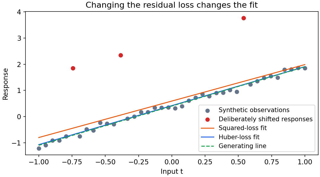
Code: fit a line with two losses
The data and shift are generated locally. The smooth optimization call follows the official SciPy interface [2]. We compare solutions and verify the robust objective’s gradient instead of asserting that one estimator always wins.
Code · Python · 23 lines
import numpy as np
from scipy.optimize import minimize

rng = np.random.default_rng(15)
t = np.linspace(-1, 1, 40)
A = np.column_stack([np.ones_like(t), t])
b = 0.4 + 1.5*t + rng.normal(0, 0.08, len(t))
b[[5, 12, 30]] += 2.5
least_squares = np.linalg.lstsq(A, b, rcond=None)[0]
delta = 0.2

def huber_objective(x):
    r = A @ x - b
    loss = np.where(abs(r) <= delta, 0.5*r*r,
                    delta*abs(r) - 0.5*delta**2)
    return loss.sum(), A.T @ np.clip(r, -delta, delta)

fit = minimize(huber_objective, least_squares, jac=True,
               method="BFGS", options={"gtol": 1e-9})
assert np.linalg.norm(huber_objective(fit.x)[1]) < 1e-6
print("squared-loss coefficients:", np.round(least_squares, 4))
print("Huber-loss coefficients:", np.round(fit.x, 4))
print("robust objective:", round(fit.fun, 6))
Uncertain operators
Suppose the matrix itself may vary in a specified set . A worst-case approximation model is
is the decision, the fixed target, and the allowed measurement matrices. Each fixed-matrix norm objective is convex in , so their pointwise supremum is convex [1, Section 6.4].
Convexity does not guarantee that evaluating this supremum is easy. A finite uncertainty set can yield finitely many epigraph restrictions. Structured ellipsoidal uncertainty can permit conic reformulations. A vaguely described “small perturbation” is not enough to select the correct counterpart.
An expected squared-error model is different. If , with , then
is the mean operator, its random variation and a positive-semidefinite second-moment matrix. The cross term vanishes under the zero-mean assumption. Here regularization follows from a specified uncertainty model, rather than an arbitrary complexity preference.
Worst-case and expected protection answer different questions. An uncertainty set is not a probability distribution. A covariance model does not promise control of every possible realization.
Function fitting with shape constraints
Plain version. We can ask a fitted function to be increasing or convex while keeping the optimization convex in its coefficients.
For fixed basis functions ,
is the input, are known basis functions, and are fitted coefficients. Evaluating at fixed sample inputs makes the predictions affine in , even when the basis functions are nonlinear in .
This distinction matters: convexity in the optimization variables is not the same as convexity in the function’s input. A polynomial regression may be a convex coefficient-fitting problem while the fitted polynomial is neither increasing nor convex.
At ordered knots , let be fitted values. Monotonicity can be imposed by . Convexity of the piecewise-linear interpolant requires
are variables and the knot spacings are fixed positive numbers. These slope-order inequalities are linear in fitted values. Unlike sampling a derivative of an arbitrary flexible function, they guarantee the shape of this particular interpolant throughout its knot interval.
Code: monotone absolute-error fitting as an LP
We fit five ordered measurements. The auxiliary variables represent absolute residual bounds. SciPy’s LP bounds are explicitly specified [3], including unrestricted fitted values.
Code · Python · 22 lines
import numpy as np
from scipy.optimize import linprog

observed = np.array([0., 2., 1., 3., 4.])
n = len(observed)
I = np.eye(n)
order = np.zeros((n-1, n))
for i in range(n-1):
    order[i, i], order[i, i+1] = 1, -1
G = np.vstack([np.hstack([I, -I]),
               np.hstack([-I, -I]),
               np.hstack([order, np.zeros((n-1, n))])])
h = np.r_[observed, -observed, np.zeros(n-1)]
fit = linprog(np.r_[np.zeros(n), np.ones(n)], A_ub=G, b_ub=h,
              bounds=[(None, None)]*n + [(0, None)]*n,
              method="highs")
assert fit.success
z = fit.x[:n]
assert np.all(np.diff(z) >= -1e-9)
assert np.isclose(abs(z-observed).sum(), fit.fun)
print("monotone fitted values:", z)
print("total absolute residual:", fit.fun)
Absolute-error solutions may be nonunique. The code verifies the property and objective rather than requiring one particular plateau value. Adding a strictly convex secondary objective would select one solution, but would be a different stated problem.
Constraints outside the observed interval require care. Piecewise-linear interpolation supplies a clear in-range function; extrapolation is an additional rule. Shape restrictions can improve plausibility while introducing bias if the underlying process violates them.
Likelihood and convex parameterizations
Plain version. A likelihood model can generate a convex objective, but the chosen parameterization and domain determine whether that is true.
For independent observations under a distribution with natural parameter ,
is a sufficient-statistic vector, the log-partition function and a parameter-independent base term. For an exponential-family model, is convex on its natural domain.
Ignoring terms independent of , the negative log-likelihood is
is the number of observations. This is convex in the natural parameter. An arbitrary nonlinear change of parameter does not necessarily preserve convexity [1, Section 7.1].
For Bernoulli observations with success probability and successes out of , the negative log-likelihood is . Its interior optimum is when both outcomes are observed.
If every observation is a success or every observation a failure, the optimum over the open domain may only be approached at a boundary. Allowing boundary distributions or adding a prior changes the existence question. A program that clips probabilities should record that clipping as a domain choice.
Maximum a posteriori estimation adds the negative log prior. A convex negative log prior preserves convexity in the selected coordinates. “Bayesian” alone does not guarantee a convex optimization problem, and a point estimate does not represent the entire posterior uncertainty.
Optional: Logistic separation and finite estimates (in the Supplementary notes). A worked example distinguishes diverging coefficients from an objective unbounded below.
Nonparametric probabilities
For discrete outcomes, estimate a probability vector on the simplex:
is the probability of outcome . Given counts , the negative log-likelihood is , with the appropriate extended-value convention for positive counts at zero probability.
Known moments become affine restrictions, such as for fixed outcome features and known mean . Maximizing entropy, equivalently minimizing , selects a distribution subject to such constraints [1, Section 7.2].
Moment restrictions should come from the same population and units as the data. Inconsistent empirical constraints can make the simplex model infeasible. Softening them adds a modeling decision about acceptable uncertainty, rather than repairing an algebraic nuisance.
Detector design as a linear program
Plain version. Choosing decisions after observing discrete evidence can be optimized directly. Allowing randomized decisions makes the feasible set convex.
Suppose is the known probability of observation under hypothesis . Let be the probability of deciding hypothesis after seeing .
is the probability of deciding when is true. is the decision variable; the conditional probabilities are fixed. Each entry of is linear in .
Weighted error costs, lower bounds on correct detection and upper bounds on false decisions can therefore be expressed as linear objectives and restrictions [1, Section 7.3]. A prior distribution on hypotheses can weight overall expected error, but should not be silently substituted for a conditional-error guarantee.
For binary hypotheses, likelihood-ratio threshold rules emerge from suitable optimal detector formulations. A boundary observation may need randomization to meet an exact error budget. Deterministic rules are a restricted subset; forcing them introduces discrete choices.
An optimized detector is only as valid as its conditional distributions. Distribution shift, estimated likelihoods and calibration uncertainty belong in the assessment. Numerical optimality under a specified probability table does not validate that table.
Worked detector: why randomization can be useful
A false-positive budget can fall between two deterministic rules. Suppose the observation is either or . Under hypothesis , its probabilities are ; under , they are . These are synthetic conditional probability tables, not measured frequencies.
Let be the probabilities of deciding after each observation. Maximizing true-positive probability with false-positive budget is the LP
Here the objective is detection probability under , and the first restriction is error probability under . Spending one unit of error budget on yields four units of detection probability, whereas spending it on yields only one quarter. Allocate the budget to : , , giving true-positive probability .
A deterministic decision on would cost , beyond the budget. With this discrete observation alphabet, every nontrivial deterministic rule violates the stated budget, so the only allowed deterministic rule always decides and detects nothing. Randomization fills the convex space between deterministic rules and achieves the desired operating point [1, Section 7.3]. This is randomizing a decision after a known observation, not treating unknown probabilities as decision variables.
Moment and exponential risk bounds
Plain version. Sometimes we know moments but not the whole distribution. Bounds can control a tail event conservatively, with assumptions stated explicitly.
For a scalar random variable with mean and finite variance , Chebyshev’s inequality gives
is a deviation threshold. The bound uses only the first two moments and can be loose. An upper bound above one can be replaced by one; it is not an estimated event probability [1, Section 7.4].
For a threshold , an exponential or Chernoff bound uses
is a positive auxiliary parameter, and the expectation must be finite where used. Optimizing its logarithm gives .
The log moment-generating function is convex in on its domain. This does not automatically make every joint design-and-risk problem convex in all its variables. Check how the random variable depends on decisions and which distribution assumptions are retained.
Tail bounds can support conservative design constraints. They do not replace checking whether moments were reliably estimated. Heavy tails, dependence and finite-sample uncertainty can make an assumed moment-generating function unsuitable.
Choosing the next measurements
Plain version. Estimation quality depends on what we measure, not only on how we fit. Convex experiment design allocates continuous measurement effort before any discrete rounding.
For candidate measurement vectors , independent unit-variance noise and normalized weights , define
is the information matrix per normalized measurement effort. The covariance of a corresponding linear estimator scales with its inverse when the matrix is positive definite, the measurement model is correct and total effort is accounted for.
D-optimal design minimizes , which targets an uncertainty-volume criterion. A-optimal design minimizes , targeting total coordinate variance. E-optimal design maximizes the smallest eigenvalue of , targeting the weakest measured direction [1, Section 7.5].
These are different scalar summaries. Units and coordinate changes can affect their interpretation differently. A small total variance may hide one poorly measured direction; a small uncertainty volume does not promise a bound on every coordinate.
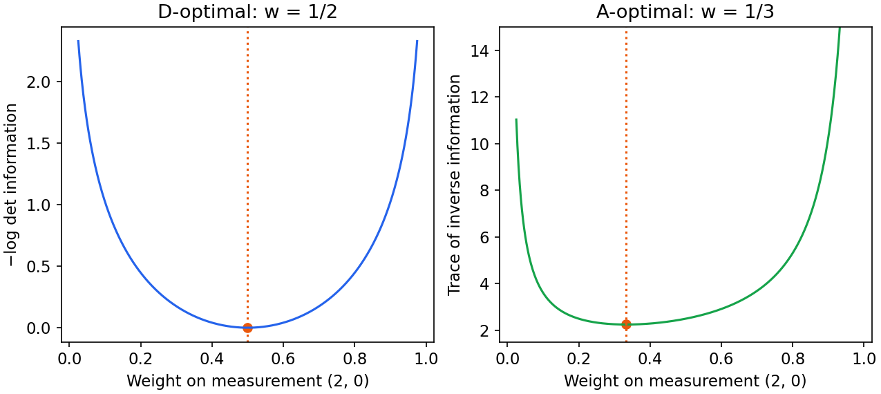
Code: two design criteria with exact checks
Use candidate vectors and , with first weight and second weight . The information matrix is diagonal: . Both criteria diverge at an unobserved direction.
Code · Python · 15 lines
import numpy as np
from scipy.optimize import minimize_scalar

def d_loss(w):
    return -np.log(4*w) - np.log(1-w)

def a_loss(w):
    return 1/(4*w) + 1/(1-w)

d = minimize_scalar(d_loss, bounds=(1e-6, 1-1e-6), method="bounded")
a = minimize_scalar(a_loss, bounds=(1e-6, 1-1e-6), method="bounded")
assert np.isclose(d.x, 0.5, atol=1e-5)
assert np.isclose(a.x, 1/3, atol=1e-5)
print("D-optimal first weight:", round(d.x, 6))
print("A-optimal first weight:", round(a.x, 6))
With a fixed number of experiments, actual counts are integers. Continuous weights are a relaxation or a randomized sampling policy. Rounding can destroy a budget or leave a direction unmeasured, so reassess the resulting matrix after converting weights into a schedule.
If candidate vectors do not span the parameter space, no weighting makes the information positive definite. Adding a prior matrix may regularize the design, but changes its interpretation to prior-plus-measurement information.
Derive why the two design criteria allocate differently
The two-direction experiment can be solved before running numerical code. With candidate vectors and and weights , its information matrix is . Let so both directions are measured.
The D-optimal objective and its derivative are
Here is the negative log-determinant criterion. Stationarity gives . The strength factor four changes the objective by a constant and does not change this D-optimal allocation.
For A-optimal design,
Here is the inverse-information trace criterion. Positive denominators turn its stationary equation into , giving . Each scalar objective has positive second derivative and diverges at the endpoints, so these stationary points are the unique global minima [1, Section 7.5].
The interpretation is useful: the first measurement already observes its direction more strongly, so minimizing total variance sends more effort to the weaker second direction. Minimizing uncertainty volume balances multiplicative directional information instead and gives equal effort. If measurement cost or noise variance differs, incorporate those changes in the information matrix and budget before repeating the derivation. Neither allocation is universally best; each answers its chosen uncertainty question.
A fitting and design audit
Start with the application quantity that must be accurate. Decide whether it is a prediction, parameter component, worst residual or a distributional probability. Then state the representation and units before selecting a numerical loss.
For each constraint, ask whether it is physically required, statistically estimated or introduced for numerical convenience. Those roles imply different responses to infeasibility. A physical limit may need a revised design; an empirical moment may need uncertainty; redundant algebra may need removal.
After fitting, verify domain membership, shape restrictions and solver residuals. Then assess generalization or uncertainty using an appropriate independent procedure. An optimum of a training objective and a reliable future prediction are separate claims.
For design, inspect the information spectrum, available budget, noise assumptions and schedule conversion. Report the final implementable schedule alongside the relaxed objective. This keeps the most consequential approximation visible.
What an uncertainty ellipsoid actually says
An inverse information matrix describes a covariance only under the corresponding measurement and estimator assumptions. Turning it into a region with a stated coverage probability needs a distributional argument and a correctly chosen threshold. Drawing an ellipse from that matrix alone does not establish a confidence level.
For a positive-definite covariance , an ellipsoid can be written as . Here is a center and is a threshold. The matrix specifies shape; the threshold specifies size. Coverage additionally depends on the actual distribution of estimation error.
A prior covariance, a sampling covariance and a numerical Hessian inverse need not have the same interpretation. They can coincide under particular models, but should not be exchanged without checking those models. Likewise, an estimator’s optimization tolerance and its sampling uncertainty have different units and sources.
When measurements are repeated, independent equal-variance assumptions justify a simple additive information model. Correlated repeats can provide less new information than their count suggests. A design that ignores that correlation may confidently allocate effort to redundant measurements.
This distinction affects stopping precision. Solving far below the uncertainty in the input coefficients may offer little practical value, while violating a hard physical bound by a seemingly small amount may still be unacceptable. Set optimization tolerances against the relevant application scale, rather than choosing precision solely from the number of available floating-point digits.
Finally, uncertainty visualization should state whether it displays an analytical model, an estimated covariance or repeated synthetic experiments. The figures in this chapter show illustrative fits and objective curves. They do not display empirically calibrated coverage regions or claim a particular confidence probability.
Modern view
Plain version. Current work combines structured convex estimation with large-scale first-order computation and learned convex components. The convexity guarantee belongs to the stated variables and domains.
Pokutta’s 2024 survey [4] organizes Frank–Wolfe methods around linear minimization over a convex feasible set, convergence guarantees and useful variants. Simplex-constrained experiment design is a natural setting for this viewpoint: an extreme-point search can avoid a full projection. The objective still needs the required smoothness and positive-definite domain control.
Schaller, Bemporad and Boyd’s 2025 manuscript [5] studies learning parametric convex functions for subsequent optimization. It connects fitting with disciplined curvature rules: a learned component can preserve convexity in decision variables for valid fixed parameters. Training the component is a separate problem and need not itself be convex.
These sources cover complementary questions: how to move through a structured feasible set, and how to construct functions usable inside such a set. Neither replaces uncertainty modeling, held-out evaluation or the physical feasibility of a design.
Current challenges include reliable uncertainty under model mismatch, informative measurements under resource limits, shape restrictions that remain appropriate outside the sample interval, and scalable updates when observations arrive sequentially. Distinguish a provably convex estimator from a complete validated statistical pipeline.
Key takeaways
- Residual norms, parameter norms and evaluation metrics answer different questions.
- Regularization weights depend on objective normalization and feature units.
- Robust residual losses and uncertain-operator models protect against different errors.
- Fixed nonlinear bases can still yield convex coefficient fitting.
- Likelihood convexity depends on parameterization and domain.
- Randomized discrete-evidence detectors can be formulated as LPs.
- Experiment-design criteria differ, and continuous weights require an implementation plan.
Exercises
- Formulate maximum absolute residual fitting as an LP, including unrestricted parameters.
Hint
Use one nonnegative residual bound.
- Scale observations and predictions by ten. Determine how a Huber transition and a quadratic regularization weight should change to preserve a chosen equivalent objective.
Hint
Write the scaled objective explicitly; the answer depends on whether parameters and penalty units are also scaled.
- Add convexity constraints to the five-knot monotone-fitting example, using unequal positive knot spacings.
Hint
Order adjacent slopes.
- Derive the Bernoulli maximum-likelihood estimate, and explain the open-domain boundary cases.
Hint
Set the likelihood derivative to zero, then inspect endpoints.
- Construct a two-hypothesis randomized detector LP with a stated false-positive budget.
Hint
Use decision probabilities per observation, and conditional error as a linear expression.
- Derive the two-direction D- and A-optimal weights in the code, then explain why rounding a small measurement budget needs another check.
Hint
Differentiate the scalar criteria; inspect whether each rounded direction receives a measurement.
References
-
Stephen Boyd and Lieven Vandenberghe, Convex Optimization, Cambridge University Press, 2004. Reading: Chapter 6, Sections 6.1–6.5; Chapter 7, Sections 7.1–7.5. Official book, free PDF.
-
SciPy developers, “scipy.optimize.minimize” and “scipy.optimize.minimize_scalar,” SciPy API documentation, accessed 2026. Multivariate interface, scalar interface.
-
SciPy developers, “scipy.optimize.linprog,” SciPy API documentation, accessed 2026. Official documentation.
-
Sebastian Pokutta, “The Frank-Wolfe Algorithm: A Short Introduction,” Jahresbericht der Deutschen Mathematiker-Vereinigung, 126, 2024. Open-access survey.
-
Michael Schaller, Alberto Bemporad and Stephen Boyd, “Learning Parametric Convex Functions,” manuscript, 2025. Official manuscript page.
-
SAS Institute, “Existence of Maximum Likelihood Estimates,” SAS/STAT 12.1 User’s Guide, accessed 2026-11-05. Official documentation.
Check your understanding
This tutorial has 6 exercises. Can you solve them without opening the hints?
Go to the exercises ↑Next OPT 06 · Gradient Descent, Newton Steps and Numerical Reliability · 19 min