OPT 02 · Convex Functions, Composition and Conjugates
Needs: OPT 01 · Modeling Decisions and Convex Sets
Navigate: this page and this track: Navigate: this page and this track
On this page
- What you’ll learn1 min
- The big picture1 min
- Chords, domains and epigraphs1 min
- Supporting planes: the first-order test2 min
- Curvature: the second-order test2 min
- A catalog of useful functions1 min
- Sums, substitutions and pointwise maxima1 min
- Composition with monotonicity2 min
- Log-sum-exp and stable evaluation1 min
- Perspectives: normalize a variable without losing convexity1 min
- Conjugates and linear lower bounds2 min
- Quasiconvexity and logarithmic structure2 min
- Modern view1 min
- Key takeaways1 min
- Exercises1 min
- References
Optimization
Explore this chapter 1 interactive experiment
Measure the Jensen gap while moving between two inputs. A negative gap supplies a concrete counterexample.
What you’ll learn
- Define convexity with domains, chords and epigraphs.
- Use first-order and second-order tests without assuming differentiability everywhere.
- Recognize important scalar, norm and matrix functions.
- Build convex models using sums, affine substitutions, maxima, composition and perspectives.
- Derive conjugates and understand their connection to linear lower bounds.
- Distinguish convex, strongly convex, quasiconvex and log-concave structure.
The big picture
The previous chapter described allowed choices. This chapter describes how their scores change. A convex objective has a useful consistency: mixing two choices cannot produce a score worse than the corresponding mixture of their scores. Its local supporting planes provide global lower bounds.
This does not mean every familiar loss is convex in every variable. Squared error is convex in the predicted values and in linear model coefficients. It is generally not convex in all parameters of a multilayer neural network. Always specify the variable being optimized and the domain being considered.
Boyd and Vandenberghe’s Chapter 3 [1] develops several ways to recognize this structure. The goal is not to memorize a huge catalog. It is to combine a small catalog with valid transformation rules, so a complicated objective comes with a reason for being convex.
Convexity is a statement about the complete function, including its domain. A formula may have positive curvature wherever defined, while its domain is disconnected. That does not define a convex function on the whole set. Domain restrictions deserve the same attention as derivatives.
Chords, domains and epigraphs
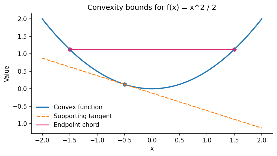
Plain version. Draw the straight line between two function values. For a convex function, the actual value at every intermediate input is no higher than that line.
For a function on convex domain ,
are arbitrary inputs, is a mixing weight, and is convex if this inequality holds for every such choice. Reversing the inequality defines concavity. An affine function satisfies equality and is both convex and concave.
The condition compares inputs and outputs simultaneously. Convexity of the domain ensures the mixed input is available. A function does not qualify by passing the inequality only for a convenient subset of endpoint pairs.
The epigraph is
is a scalar vertical coordinate and is a point above or on the function graph. A function is convex exactly when its epigraph is a convex set. This provides a bridge from Chapter 1’s geometry to objectives and inequality constraints.
An epigraph formulation introduces a variable and minimizes it subject to . It can make a nonsmooth objective easier to express using constraints. It does not change the mathematical optimum when the formulation is exact.
Jensen’s inequality and expectations
The two-point inequality extends to finite weighted averages:
are inputs and are weights. For a random vector with suitable integrability and domain conditions, the analogous statement is .
This explains why a convex cost applied after averaging can be smaller than the average individual cost. It does not say that averaging arbitrary model parameters improves prediction: the prediction function and its loss must be convex in those parameters for that conclusion.
Jensen’s inequality also helps reason about risk and uncertainty. A nonlinear transformation of an expected measurement need not equal the expected transformed measurement. The direction depends on convexity or concavity, not on a vague claim that averages are always representative.
Supporting planes: the first-order test
Plain version. For a differentiable convex function, the tangent approximation is a global lower bound, not merely a local sketch.
On an open convex domain, differentiable convexity is equivalent to
is the point where the approximation is made, is any domain point, and is the gradient with respect to the optimization variable. The affine expression on the right supports the function from below.
One way to derive the inequality is to apply the convex chord rule at , rearrange it, divide by positive and let tend to zero. This turns a global mixing condition into a directional derivative bound.
If , the supporting-plane inequality gives everywhere in the domain. Thus a stationary point is globally minimizing in an unconstrained differentiable convex problem. It need not be unique.
With constraints, a nonzero gradient can still be optimal because improving directions are disallowed. The duality and constrained-algorithm chapters express that fact precisely. Simply requiring a small gradient is not an appropriate stopping rule for every constrained problem.
Nonsmooth supporting vectors
A corner does not destroy convexity. For convex , a subgradient at satisfies
is a vector supplying a supporting affine lower bound; the set of all such vectors is the subdifferential . At a differentiable point it contains only the gradient. At the origin, the absolute-value function has all scalar subgradients in .
The notation is useful for absolute residuals, maxima and sparsity penalties. A subgradient is not an ordinary derivative chosen arbitrarily at a corner: it must satisfy a global support inequality. Later chapters use this structure when discussing proximal methods.
For a convex unconstrained function, implies global optimality. A zero gradient and a zero included among many subgradients therefore express the same underlying support idea in different settings.
Curvature: the second-order test
Plain version. A smooth function is convex when it bends upward in every direction. Looking at only one coordinate at a time can miss a downward diagonal direction.
For twice continuously differentiable on an open convex domain,
is equivalent to convexity. is the symmetric Hessian matrix, and means every directional quadratic form is nonnegative.
Nonnegative diagonal Hessian entries are insufficient. The function has zero coordinate second derivatives but an indefinite Hessian. Along one diagonal it curves upward, along the other downward.
The test is a global condition on the entire domain. Evaluating eigenvalues at ten points is a numerical diagnostic, not a proof. A symbolic Hessian with an analytical positive-semidefinite factorization can establish the property for all points.
Strict and strong convexity
Strict convexity requires a strict chord inequality for distinct endpoints and weights strictly between zero and one. When a minimum exists on a convex set, strict convexity ensures uniqueness.
Strong convexity in the Euclidean norm requires, for some ,
is a uniform curvature lower bound. For twice differentiable functions, it corresponds to , where is the identity matrix. Strong convexity is stronger than strict convexity; a function can be strictly convex without a positive uniform curvature bound.
Adding a positive quadratic regularizer often supplies strong convexity in the penalized coordinates. An unpenalized intercept or a restricted domain requires separate analysis. Do not infer strong convexity of every parameter merely from one regularization term.
What the Hessian test measures
A multivariable curvature test becomes a scalar test along every line. Fix a point and direction , and set on the interval that stays in the domain. Differentiating twice gives
Here is the line coordinate, the restricted scalar function, and any direction. A positive-semidefinite Hessian makes every such restriction convex. Every segment is part of one of these lines, so the chord definition follows. Conversely, convexity on every line requires its second derivative to be nonnegative. This explains why the test examines quadratic forms in all directions rather than individual matrix entries [1].
Strict and strong convexity differ in a concrete example. The scalar function is strictly convex on : its derivative is strictly increasing. Yet , so no positive global satisfies the strong-convexity Hessian bound. Its minimum is unique, but the strong-convexity stopping bound in OPT 06 is unavailable. Adding , with chosen , supplies the missing curvature floor and changes the objective.
A catalog of useful functions
Plain version. A few familiar building blocks cover a large share of practical convex objectives. Their domains and signs determine how they can be used.
Affine functions are both convex and concave. Norms are convex because of positive homogeneity and the triangle inequality. Squared Euclidean norm is convex and smooth; the norm itself is nonsmooth at the origin.
A quadratic
is convex exactly when symmetric . Here sets curvature, is a linear coefficient vector and is a scalar constant. Positive-definite gives strong convexity with a bound set by its smallest eigenvalue.
Scalar exponential is convex everywhere. Negative logarithm is convex on positive inputs. Powers need their exponent and domain specified; statements such as “all power functions are convex” are false. For example, square root is concave on nonnegative inputs, while its negative is convex there.
The maximum coordinate and maximum of affine scores are convex and generally nonsmooth. A minimum of affine functions is concave, not generally convex. The sign of a modeling expression is therefore important.
Matrix-valued domains
The function is convex for positive-definite symmetric matrices [1, Section 3.1]. The variable is a matrix, and the domain excludes singular matrices.
For a symmetric perturbation , its second directional derivative is
is a direction in the space of symmetric matrices and is trace. After a congruence transformation this becomes a squared Frobenius norm, explaining the nonnegative curvature.
The largest eigenvalue of a symmetric matrix is convex because
denotes the largest eigenvalue and ranges over unit vectors. Each quadratic form is affine in the matrix entries of , so their pointwise supremum is convex. This is a useful example of analyzing which quantity is the variable.
Code: Hessian checks for a quadratic and a counterexample
This code checks constant Hessians, so the eigenvalue test applies at every input. It also verifies one supporting-plane inequality numerically.
Code · Python · 14 lines
import numpy as np

Q = np.array([[3.0, 1.0], [1.0, 2.0]])
bad = np.array([[0.0, 1.0], [1.0, 0.0]])
assert np.linalg.eigvalsh(Q).min() > 0
assert np.linalg.eigvalsh(bad).min() < 0
x, y = np.array([0.4, -0.6]), np.array([-1.0, 0.8])
f = lambda z: 0.5 * z @ Q @ z
support = f(x) + (Q @ x) @ (y - x)
gap = f(y) - support
assert np.isclose(gap, 0.5 * (y - x) @ Q @ (y - x))
print("quadratic Hessian eigenvalues:", np.linalg.eigvalsh(Q))
print("product Hessian eigenvalues:", np.linalg.eigvalsh(bad))
print("supporting-plane gap:", gap)
Sums, substitutions and pointwise maxima
Plain version. Build a complicated objective from known functions through operations that preserve convexity. The preservation rule is the proof.
A nonnegative weighted sum of convex functions is convex. Negative coefficients generally reverse or destroy the property. An integral or expectation of convex functions is convex when the result is well-defined and the distribution is fixed independently of the decision variable.
Affine substitution preserves convexity:
is convex, is a fixed matrix and a fixed vector. The domain of contains points whose transformed values lie in the domain of . This rule establishes convexity of squared residuals, norm residuals and many regularized linear estimators.
If are convex, then is convex on their common domain. An epigraph variable expresses this as for every . This models the worst residual, worst scenario cost or maximum coordinate without needing a smooth objective.
An infimum over a jointly convex auxiliary variable also preserves convexity under the appropriate formulation:
is jointly convex in and is the eliminated variable. Joint convexity matters; convexity in each block separately is insufficient. This rule connects partial minimization with the projection of an epigraph.
What does not automatically preserve convexity
Products of convex functions are not generally convex. Dividing one convex function by another is not generally convex. Taking a minimum of convex functions can create multiple valleys.
For example, is not jointly convex merely because it is a product of two nonnegative convex expressions. A reciprocal or exponential outside an expression needs a composition argument with the right monotonicity. Mathematical plausibility is not a substitute for checking a rule.
Multiplying a fixed parameter by a variable is affine. Multiplying two decision variables is bilinear and generally nonconvex. Many modeling errors arise from accidentally treating a learned or unknown quantity as if it were fixed.
Composition with monotonicity
Plain version. An outer convex function can preserve convexity when it reacts to each inner argument in the right direction.
Suppose
is an outer function and are scalar inner functions. A standard sufficient rule is: is convex, and for each argument it is nondecreasing when is convex, nonincreasing when is concave, or the inner function is affine. Domain conditions and the appropriate extended-value interpretation are included in the rule [1, Section 3.2].
For instance, exponential is convex and increasing, so exponentiating a convex inner expression preserves convexity. Negative logarithm is convex and decreasing, so applying it to a positive concave inner expression gives a convex function.
The monotonicity qualifier cannot be omitted. Squaring a convex expression is not always convex because square is decreasing on negative inputs and increasing on positive ones. Squaring a nonnegative convex expression is a valid composition, while arbitrary signs require another argument.
These are sufficient recognition rules, not a complete decision procedure for every algebraic expression. An expression may be convex even though its current syntax fails the rules. Rewriting as a Euclidean norm exposes convexity directly.
A composition rule seen through derivatives
For scalar smooth functions, the chain rule shows where the monotonicity requirement enters. Set . Then
Here primes denote scalar derivatives, is the inner function and the outer function. If is convex and nondecreasing and is convex, both terms are nonnegative. If is convex and nonincreasing while is concave, the second term is again nonnegative. Composition rules also handle nonsmooth functions, but this calculation exposes the signs [1].
Take the convex inner expression and the convex outer function . Their composition is , whose second derivative is . It is negative at zero, so the composition is nonconvex. The inner output is negative near zero, where the square function is decreasing; the required sign agreement fails.
When the domain is convex and a convex inner expression is nonnegative throughout it, squaring is valid because the outer function is nondecreasing there. This is why squared Euclidean residual norms are convex but “square any convex loss expression” is not a valid general rule.
Log-sum-exp and stable evaluation
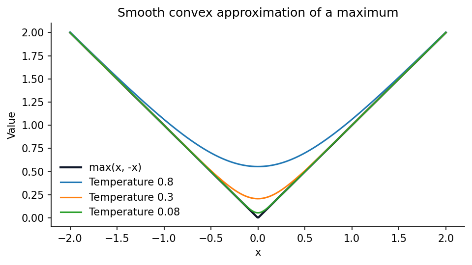
Plain version. Log-sum-exp is a smooth upper approximation to the largest score. It also provides the normalization behind probability-like weights.
For ,
are scalar coordinates; are normalized positive weights summing to one. Its gradient is and its Hessian is
places the weights on a diagonal. For any direction , the quadratic form is the weighted variance of , which is nonnegative. This proves convexity.
Adding the same constant to every coordinate shifts the function by that constant. The all-ones direction therefore has zero Hessian curvature; the function is not strongly convex on the entire space.
For temperature , define . Then
controls smoothness and the approximation error. A small temperature approaches the maximum but can make numerical optimization less well-conditioned. Stable evaluation subtracts the largest scaled coordinate before exponentiating.
Code: stable log-sum-exp and a Jensen check
This example avoids overflow at large inputs, verifies the Hessian and illustrates one finite Jensen comparison.
Code · Python · 16 lines
import numpy as np
from scipy.special import logsumexp

x = np.array([1000.0, 999.0, 997.0])
value = logsumexp(x)
p = np.exp(x - value)
H = np.diag(p) - np.outer(p, p)
assert np.linalg.eigvalsh(H).min() >= -1e-12
assert np.isclose(p.sum(), 1)
u, v = np.array([1., -1., 0.]), np.array([-2., 2., 1.])
theta = 0.3
left = logsumexp(theta * u + (1 - theta) * v)
right = theta * logsumexp(u) + (1 - theta) * logsumexp(v)
assert left <= right + 1e-12
print("stable value:", value, "weights:", p)
print("Jensen gap:", right - left)
Perspectives: normalize a variable without losing convexity
Plain version. A perspective combines a cost at a normalized input with the amount of scale used. This creates useful convex expressions that look like ratios.
For convex , its perspective is
is a vector, a positive scalar scale and is jointly convex in both variables. The positive-scale domain is essential.
Taking gives . This quadratic-over-linear function is jointly convex, even though arbitrary ratios are not.
The rule can be proved by mixing two pairs and , then recognizing that their normalized input is a convex combination with weights proportional to and . Apply convexity of and multiply by the combined positive scale.
Perspective formulations arise when cost depends on a normalized rate, allocated duration or positive mass. They can also reveal exact conic representations. Keep physical meaning and domain constraints visible: permitting zero or negative scale without a careful closed extension changes the function.
Perspective proof: the weights change after normalization
Ordinary averaging does not commute with division by a variable scale. The perspective remains convex because normalization produces a different, still valid pair of weights.
Take two domain points with and mixing weight . Define
Here are the mixed numerator and scale; is the normalized weight. Apply convexity of to the last line and multiply by . The coefficients become and , giving exactly the convex chord bound for [1].
For the quadratic-over-linear example, take and with . Their costs are and . The mixed point costs , below their average . Its normalized input is , obtained with weight on the first normalized input and on the second . The scale-dependent weights are the key step; simply averaging the normalized inputs would give a different number.
Conjugates and linear lower bounds
Plain version. A conjugate asks how much an arbitrary linear score can exceed a function. The answer describes the tightest intercept for a supporting line with that slope.
The convex conjugate is
is a candidate slope vector, is the original variable and is the supremum gap. A finite conjugate value yields the global lower bound
This follows immediately from the supremum definition and is the Fenchel inequality [1, Section 3.3]. Conjugates are useful for deriving dual problems and splitting algorithms.
For with positive-definite , maximizing the gap gives . Therefore
is the quadratic curvature matrix. In numerical code solve rather than explicitly inverting .
The conjugate of an indicator of a set is its support function. An extended-value indicator is zero on the allowed set and positive infinity elsewhere. This makes a constraint part of an objective without using a finite penalty.
For proper closed convex functions, conjugating twice recovers the original function. These regularity conditions matter: without them, the double conjugate describes the appropriate closed convex envelope rather than blindly reproducing every original formula.
Code: a conjugate certificate
Equality holds in the quadratic Fenchel bound at the matching slope . The code checks both equality and a nonnegative gap elsewhere.
Code · Python · 13 lines
import numpy as np

Q = np.array([[4., 1.], [1., 2.]])
x = np.array([0.5, -0.8])
y = np.array([1.2, 0.3])
f = lambda z: 0.5 * z @ Q @ z
conjugate = lambda slope: 0.5 * slope @ np.linalg.solve(Q, slope)
gap = f(x) + conjugate(y) - x @ y
matching = Q @ x
assert gap >= -1e-12
assert np.isclose(f(x) + conjugate(matching), x @ matching)
print("Fenchel gap:", gap)
print("matching slope:", matching)
A nonsmooth conjugate with a visible domain
The conjugate can turn a nonsmooth penalty into a simple restriction on slopes. Let with fixed . Separating the coordinates in its definition gives
Here are coordinates of the original variable and slope; . When , each coordinate expression is at most zero, attained at . When one slope exceeds that threshold in magnitude, choosing with its sign and increasing magnitude makes the expression unbounded.
Thus the domain of the conjugate is an infinity-norm ball. The corresponding lower bound is tight when nonzero coordinates have matching slopes . This links norm geometry, subgradients and dual feasibility in one calculation [1, Section 3.3]. OPT 08 uses the same threshold structure to derive a proximal update.
Quasiconvexity and logarithmic structure
Plain version. Some functions are not convex, but every set of inputs below a chosen score is convex. Other functions become convex or concave after taking a logarithm. These are useful structures with different guarantees.
A function is quasiconvex if all sublevel sets are convex:
is any real threshold and is its sublevel set. Equivalently, values at mixed inputs do not exceed the larger endpoint value. This is weaker than the convex chord inequality.
Every convex function is quasiconvex. A monotone scalar function on an interval is quasiconvex even when its curvature is not consistently upward. Under appropriate formulations, quasiconvex minimization can use bisection on a threshold and solve a convex feasibility problem at each step [1, Sections 3.4 and 4.2].
For positive , log-convexity means is convex; log-concavity means is concave. Positivity and the domain are part of these definitions. A density with concave log density has log-concave structure, but that does not make every parameter-estimation problem involving it convex in every parameterization.
Some geometric programs become convex after substituting logarithms of positive variables. This is an exact variable transformation in a specified problem class, not permission to take logarithms of arbitrary objectives and constraints. The next chapter derives the relevant form.
Convexity of a formula versus convexity of an implementation
A mathematically convex expression can be evaluated poorly. Overflow in an exponential, rounding near a matrix boundary or an accidentally broadcast array can invalidate the computed quantity while leaving the intended function convex.
Keep a symbolic curvature argument and a numerical evaluation check as separate evidence. A Hessian sampled at a few points may reveal a counterexample, but cannot prove nonnegative curvature everywhere. A stable implementation likewise does not prove the intended expression is convex.
When parameters are fixed during a solve, the convexity claim concerns decision variables at those fixed parameter values. A coefficient changing sign can invalidate a composition rule. Record which parameter ranges preserve the claim, rather than calling an entire parameterized family convex without qualification.
The same distinction applies to a learned function. Convexity in an input used later as a decision variable does not establish convexity in the weights being trained. Curvature rules describe one optimization problem at a time.
Modern view
Plain version. Convexity-preserving design is still useful when functions are learned from data. A learned function can be constrained to remain convex in its decision input without being convex in its training parameters.
Disciplined convex programming [2] formalizes composition rules so a model carries a recognizable convexity argument. The taxonomy separates affine, convex and concave expressions, tracks monotonicity and respects domains. Failing a syntactic rule can mean a reformulation is needed; it does not automatically disprove mathematical convexity.
Schaller, Bemporad and Boyd’s 2025 manuscript on learning parametric convex functions [3] studies fitting functions that remain convex in the variable for valid parameter values and are compatible with disciplined programming. It supports a specific modern connection: learning a component of an optimization model while preserving decision-variable convexity. It is an original research manuscript, not a review or a guarantee about unrestricted neural losses.
Pokutta’s 2024 survey [4] organizes constrained smooth methods around geometric access and uses convexity, smoothness and strong convexity to analyze updates. Its practical lesson is to keep curvature assumptions separate: global convexity, uniform lower curvature and an upper smoothness bound play different roles.
Open problems include choosing useful structured function classes without losing expressiveness, certifying domains under noisy learned parameters, handling nondifferentiable solution maps, and evaluating generalization of learned models. An optimization certificate proves a property of the fitted objective; it does not prove that the objective matches future observations.
Key takeaways
- Convexity includes a convex domain and a chord inequality.
- Tangents and subgradients give global lower bounds.
- Positive-semidefinite Hessians establish smooth convexity in every direction.
- Strict convexity, strong convexity and smoothness are different assumptions.
- Composition rules need monotonicity, signs and domains.
- Perspectives and conjugates expose useful structure hidden in ratios and constraints.
- Quasiconvex and log-convex formulations require their own reasoning.
Exercises
- Prove the first-order supporting-plane inequality from the chord definition for differentiable functions.
Hint
Rearrange the chord inequality, divide by the mixing weight and take its limit to zero.
- Show why nonnegative Hessian diagonal entries do not prove convexity, using a two-variable example.
Hint
Use and test diagonal directions.
- Reformulate to make its convexity visible through a norm.
Hint
Write the norm of .
- Derive the perspective of squared Euclidean norm and identify its domain.
Hint
Substitute and multiply by positive .
- Derive the conjugate of and find when Fenchel’s inequality is equality.
Hint
Maximize the quadratic gap by differentiation.
- Give a quasiconvex function on an interval that is not convex, and verify its sublevel sets.
Hint
A monotone concave function such as square root on positive inputs has interval sublevel sets.
References
- Stephen Boyd and Lieven Vandenberghe, Convex Optimization, Cambridge University Press, 2004. Reading: Chapter 3; Section 4.2 for quasiconvex feasibility. Official book page, free official PDF.
- Michael Grant, Stephen Boyd and Yinyu Ye, “Disciplined Convex Programming,” in Global Optimization: From Theory to Implementation, Springer, 2006. Author’s publication page.
- Michael Schaller, Alberto Bemporad and Stephen Boyd, “Learning Parametric Convex Functions,” manuscript, June 2025. Verified manuscript page.
- Sebastian Pokutta, “The Frank-Wolfe Algorithm: A Short Introduction,” Jahresbericht der Deutschen Mathematiker-Vereinigung, 126, 2024. Open-access survey.
Check your understanding
This tutorial has 6 exercises. Can you solve them without opening the hints?
Go to the exercises ↑Next OPT 03 · Linear, Quadratic, Conic and Geometric Programs · 18 min