OPT 07 · Equality Constraints and Interior-Point Methods
Needs: OPT 06 · Gradient Descent, Newton Steps and Numerical Reliability
Navigate: this page and this track: Navigate: this page and this track
On this page
- What you’ll learn1 min
- The big picture1 min
- 1. Equality constraints change the permitted directions3 min
- 2. A constrained quadratic with an inspectable certificate1 min
- 3. Inequalities become a smooth interior problem1 min
- 4. The central path links interior points to dual bounds2 min
- 5. A complete one-dimensional barrier experiment1 min
- 6. Feasibility, strict feasibility and Phase I2 min
- 7. Primal–dual steps and reliable stopping2 min
- 8. Interpret a certificate at the application boundary2 min
- Modern view2 min
- Key takeaways1 min
- Exercises1 min
- References
Optimization
Explore this chapter 1 interactive experiment
Raise the barrier weight t on a two-variable linear program and watch the central point, its dual bound and the gap m/t.
What you’ll learn
- Extend Newton’s method to a convex objective with affine equalities.
- Derive a logarithmic barrier, its central path and the associated duality gap.
- Implement a small feasible barrier solver with an explicit line search.
- Distinguish feasible, strictly feasible and infeasible constraint systems.
- Interpret primal–dual residuals, complementarity and infeasibility certificates.
- Compare modern interior-point and first-order solver designs using their numerical demands.
The big picture
Constraints describe what a solution is allowed to do. A solver cannot ignore them while improving the objective. Equality constraints restrict every permitted step to a lower-dimensional space; inequality constraints create boundaries the solver must handle. Interior-point methods approach useful boundary solutions through a sequence of problems whose iterates remain inside those boundaries.
The reading is Boyd and Vandenberghe, Chapters 10–11 [1]. Chapter 10 treats equality-constrained minimization; Chapter 11 develops barriers, the central path, initialization and primal–dual methods. Read them after gradient and Newton methods and return to duality and optimality when a certificate seems mysterious. Bubeck’s algorithmic monograph [2] supplies a complementary view of complexity and solver families.
This chapter uses synthetic low-dimensional problems so you can check every claim independently. The code is a teaching implementation, with assertions and transparent assumptions. A production conic solver adds scaling, sparse factorizations, numerical regularization, termination policies and infeasibility handling. Understanding the small problem helps explain those engineering choices.
1. Equality constraints change the permitted directions
An affine equality must remain satisfied while the objective decreases. If the current point satisfies , a step preserves feasibility exactly when . This gives a geometric explanation before any matrix derivation: permitted steps lie in the nullspace of the equality matrix.
Consider the convex problem
Here is the variable; is a twice-differentiable convex objective; is fixed; and is fixed. We initially assume has independent rows and the equality system has a solution. The Lagrange multiplier accounts for the equality restriction.
At a feasible iterate, minimize the quadratic approximation along feasible directions. The resulting Newton system is
Here is the Hessian; is the proposed primal step; is the equality multiplier of the local quadratic subproblem; and the zero block has size . The second block equation enforces . The multiplier solves the local model; it is not automatically the increment of a separately maintained multiplier estimate.
The Hessian need only have positive curvature along nonzero feasible directions to make the constrained quadratic model well behaved. A direction excluded by the equalities need not have positive curvature. This distinction explains why a full Hessian can be singular while the constrained minimizer is unique. Check the actual feasible subspace before diagnosing singularity as nonuniqueness.
The block matrix is a Karush–Kuhn–Tucker, or KKT, matrix [1]. It is generally indefinite even when is positive definite. Do not apply a positive-definite factorization to the entire matrix merely because the original objective is convex. Its structure reflects simultaneous primal and dual equations. For a small dense example, a general linear solve is adequate.
An alternative eliminates equalities. Choose one feasible point and a matrix whose columns span the nullspace of . Write , where is the reduced variable. Then solve the unconstrained problem in . Elimination can simplify a tiny problem but destroy sparsity in a large one. Both formulations express the same geometry; the computational representation determines the cost.
Reduced curvature and block elimination
A singular Hessian need not make the constrained step ambiguous. Minimize under . The Hessian is , but the only feasible directions change . The unique minimizer is : the equality removes precisely the flat direction.
More generally, let contain independent columns spanning the nullspace of . The reduced Hessian is . Positive definiteness of this smaller matrix gives a unique local quadratic minimizer along feasible directions, even when is singular. Here is the current Hessian and the full-row-rank equality matrix [1, Chapter 10].
If itself is positive definite, the KKT step can also be derived by eliminating the primal direction. Write and use the first block equation:
Here is the step and the local equality multiplier. The second line follows by substituting the first into . The smaller matrix is positive definite when has independent rows: for nonzero , its quadratic form is .
These equations explain the block solve, but the inverse notation is algebraic. Compute products through solves with and compare the cost of this elimination with a direct sparse KKT factorization. In the singular example above, the nullspace formulation remains valid while this full-Hessian elimination does not.
2. A constrained quadratic with an inspectable certificate
A quadratic objective makes the KKT equations exact rather than approximate. Solving the block system produces a candidate; checking equality feasibility and stationarity determines whether the candidate is an optimality certificate for this convex problem.
For
is a symmetric positive-semidefinite matrix, is fixed, and is the variable. An optimal pair satisfies and . The superscript star denotes an optimal value. These equations are sufficient for a feasible convex quadratic; uniqueness requires additional curvature on feasible directions.
Code · Python · 17 lines
import numpy as np

Q = np.diag([2.0, 4.0])
c = np.array([-2.0, -1.0])
A = np.array([[1.0, 1.0]])
b = np.array([1.0])
K = np.block([[Q, A.T], [A, np.zeros((1, 1))]])
solution = np.linalg.solve(K, np.concatenate([-c, b]))
x, nu = solution[:2], solution[2:]
primal = A @ x - b
dual = Q @ x + c + A.T @ nu
print("Primal solution:", x)
print("Equality multiplier:", nu)
print("Residual norms:", np.linalg.norm(primal), np.linalg.norm(dual))
assert np.allclose(x, [5/6, 1/6])
assert np.linalg.norm(primal) < 1e-12
assert np.linalg.norm(dual) < 1e-12
The coordinates sum to one. The unconstrained optimum would have coordinates one and one quarter, so it would violate the total constraint. The multiplier adjusts the stationarity equation to account for that restriction. A small objective value alone would not establish this adjustment; the residual checks make it explicit.
Residuals depend on units. Multiplying the equality by a large constant leaves the feasible set unchanged while changing the raw primal residual and multiplier scale. Report the units and scaling of the original constraints, and compare residuals against meaningful tolerances. A solver’s internal normalized stopping test should be translated back into the application’s measurements.
Do not form a matrix inverse to compute this solution. A linear solve is more direct and usually more stable. In a repeated problem, factorization reuse can reduce work, but only when the matrix structure permits it. Updating a linear term is different from updating the Hessian or the constraint matrix; distinguish these changes when planning warm starts and caching.
For nonlinear objectives, recompute the local curvature and use a feasible line search. A full Newton step can leave the objective’s domain even if it preserves the equalities. The domain is an additional restriction: a logarithm or a positive-definite matrix variable is not defined everywhere. The equality equations alone do not protect it.
3. Inequalities become a smooth interior problem
A boundary can be represented by a barrier that grows without bound as the iterate approaches it. The barrier is finite only at strictly feasible points. This lets a smooth constrained Newton method handle the inequality through the objective, while retaining explicit affine equalities.
Consider convex inequalities for , with affine equalities . Define
Here is the original convex objective; each is a convex inequality function; is the number of scalar inequalities; is the logarithmic barrier; and controls the relative importance of the objective. The domain requires every . The barrier problem minimizes subject to .
Constraint functions should be expressed consistently in chosen units, or normalized by a positive reference scale before taking a logarithm. Positive rescaling changes the barrier by an additive constant and does not change its minimizer, although finite-precision calculations can still be affected. The mathematical invariance is not a reason to neglect numerical scaling.
For a twice-differentiable inequality, its barrier contribution has gradient and Hessian
Here is the gradient column vector and is its Hessian. Both terms are positive semidefinite in the strictly feasible domain because is convex. The expression also shows rapidly increasing curvature near an active boundary, where becomes small.
An inequality representation affects the path. Repeating an identical constraint repeats its barrier contribution, changing the approximate problem for finite . The exact feasible set remains unchanged. This illustrates an important separation: equivalent constraint sets need not produce identical intermediate iterates. Canonicalization and scaling are algorithmic decisions with observable effects.
The barrier cannot begin on the boundary. If a nonnegative variable starts at zero, is undefined. Use a strictly positive initialization or reformulate a variable that is forced to zero by equalities. Adding an arbitrary positive offset to a constraint changes the optimization problem and must not be mistaken for an innocuous implementation fix.
4. The central path links interior points to dual bounds
For each barrier weight, solve the interior problem accurately. The resulting minimizers form the central path. Increasing the weight weakens the barrier relative to the original objective, allowing the solution to approach a constrained optimum on the boundary.
Let minimize subject to . Define
Here is the inequality multiplier; is the equality multiplier for the scaled barrier problem; and is the multiplier in the original objective’s scale. The variables , and retain their definitions above.
Barrier stationarity becomes original Lagrangian stationarity, while complementarity becomes . Each scalar inequality contributes the same positive product. At a true optimum, complementary slackness requires those products to vanish; the barrier path approaches that condition as increases.
For an exactly centered point satisfying the stated assumptions, the associated primal–dual gap is
Here is the Lagrange dual function, a lower bound on the optimal objective for dual-feasible multipliers. The gap bounds objective suboptimality because the primal value is an upper bound and the dual value is a lower bound. This is a statement about the formulated convex problem, not a guarantee that the formulation matches the application.
The equality requires exact centering and a valid dual construction. A numerical iterate with a large stationarity residual cannot claim an exact gap merely by printing . Use the theoretical quantity to plan the barrier schedule, then check the actual residuals and, where available, evaluate a genuine dual lower bound. This prevents an outer-loop counter from masquerading as a certificate.
An outer barrier method therefore alternates two activities: solve a fixed- interior problem, then increase . Reuse the previous solution as the next starting point. The next problem usually has a nearby minimizer, but very large changes in can make centering expensive. Choose the increase based on measured centering behavior rather than assuming that fewer outer iterations always mean less computation.
Where the gap actually comes from
The central-path gap is a sum of explicit prices times explicit slacks. At an exactly centered point, divide barrier stationarity by :
Here minimizes the barrier problem, is its equality multiplier, are the original objective and inequalities, and is the barrier weight. Substituting the defined and makes this exactly the original Lagrangian’s stationarity equation.
The Lagrangian is convex in because the original functions are convex and the inequality multipliers are nonnegative. Stationarity therefore makes its global minimizer, so evaluating at this point really computes the dual function. Equality feasibility removes the equality term, giving
Here is the dual function and the scalar inequality count. The gap follows by subtracting this lower bound from the feasible primal objective. The central point is usually not the original optimizer: it trades objective improvement against positive slack. Its multipliers already supply a certificate whose error decreases as the barrier weakens [1, Section 11.2].
For a desired theoretical gap at most , choose and then solve the centering problem accurately enough. The choice of supplies a target; the stationarity solve is what justifies using the formula. Increasing without centering omits the key equality in the proof.
5. A complete one-dimensional barrier experiment
Use a constrained quadratic whose true optimum is easy to check. We minimize subject to . The unconstrained minimizer is two; the closest permitted point is one, with objective one half. A barrier solution stays strictly between zero and one and approaches the upper endpoint.
For this example,
Here is the scalar variable and is the objective weight. The first and second derivatives are and . Every denominator is positive in the barrier domain.
Code · Python · 36 lines
import numpy as np

def center(t, x):
    def value(z):
        return 0.5*t*(z-2)**2 - np.log(z) - np.log1p(-z)
    for _ in range(100):
        grad = t*(x-2) - 1/x + 1/(1-x)
        hess = t + 1/x**2 + 1/(1-x)**2
        step = -grad/hess
        if grad*grad/hess < 1e-16:
            break
        alpha = 1.0
        for _ in range(100):
            trial = x + alpha*step
            if 0 < trial < 1 and value(trial) <= value(x) + 0.01*alpha*grad*step:
                break
            alpha *= 0.5
        else:
            raise RuntimeError("Line search failed")
        x = trial
    else:
        raise RuntimeError("Centering iteration limit reached")
    return x
x = 0.5
for t in [1., 4., 16., 64., 256., 1024.]:
    x = center(t, x)
    lower, upper = 1/(t*x), 1/(t*(1-x))
    stationarity = x-2-lower+upper
    primal = 0.5*(x-2)**2
    dual = 2-upper-0.5*(-2-lower+upper)**2
    gap = primal-dual
    print(int(t), round(x, 6), round(gap, 7), round(2/t, 7))
    assert 0 < x < 1
    assert abs(stationarity) < 1e-5
    assert abs(gap-2/t) < 1e-8
    assert primal-0.5 <= gap + 1e-8
The feasible backtracking check runs before the objective comparison. This prevents logarithms from being evaluated outside their domain. The sufficient-decrease test uses the directional derivative, and the Newton decrement supplies the centering test. Maximum iteration counts turn an unexpected failure into an explicit error instead of an infinite loop.
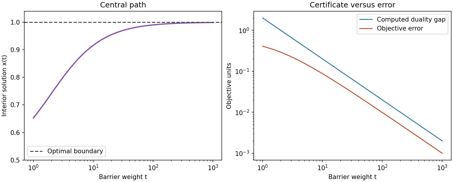
The experiment computes a genuine dual value using the unconstrained minimum of the scalar Lagrangian. It therefore checks the gap separately from the prescribed . In a larger nonlinear problem, evaluating the dual function may itself require another optimization. A primal–dual residual test is then useful, but describe what it certifies and under which regularity assumptions.
Near the endpoint, 1-x becomes small and the barrier Hessian becomes large. A smaller error target can make the numerical system harder even though the mathematical problem is unchanged. Stop when the solution is accurate enough in meaningful units. Demanding every last representable digit can waste work or expose conditioning that the application never needed to resolve.
6. Feasibility, strict feasibility and Phase I
A feasible solution may exist without any strictly feasible solution. A barrier for the original inequality representation then has no domain. This is different from infeasibility, and a solver must distinguish the two cases before trying to follow a central path.
A simple Phase I construction introduces one scalar and solves
Here bounds the largest inequality violation and is an additional variable. A point with is strictly feasible for the original inequalities. A certified positive lower bound on the optimal proves infeasibility. An optimal value zero can mean boundary-only feasibility; nonattainment and numerical uncertainty require separate attention. Finite iteration failure does not itself prove any of these outcomes.
For the contradictory system and , the violation measure is . Its minimum is one half at . Equal nonnegative weights on the two inequalities also produce an explicit infeasibility certificate.
Code · Python · 18 lines
import numpy as np

A = np.array([[1.0], [-1.0]])
b = np.array([0.0, -1.0])
y = np.array([0.5, 0.5])
print("A transpose y:", A.T @ y)
print("b transpose y:", b @ y)
assert np.all(y >= 0)
assert np.allclose(A.T @ y, 0)
assert b @ y < 0
# If A x <= b existed, multiplying by y would imply 0 <= b@y < 0.
grid = np.linspace(-1, 2, 301)
violation = np.maximum(grid, 1-grid)
assert np.isclose(violation.min(), 0.5)
# A different system is feasible only on its boundary.
A_boundary = np.array([[1.0], [-1.0]])
b_boundary = np.zeros(2)
assert np.all(A_boundary @ np.array([0.0]) <= b_boundary)
The grid is an illustration of the already derived minimum, rather than a proof that an arbitrary optimization is globally solved. The certificate is the decisive argument: if , multiplying by would imply , a contradiction. The certificate checks data and multipliers directly.
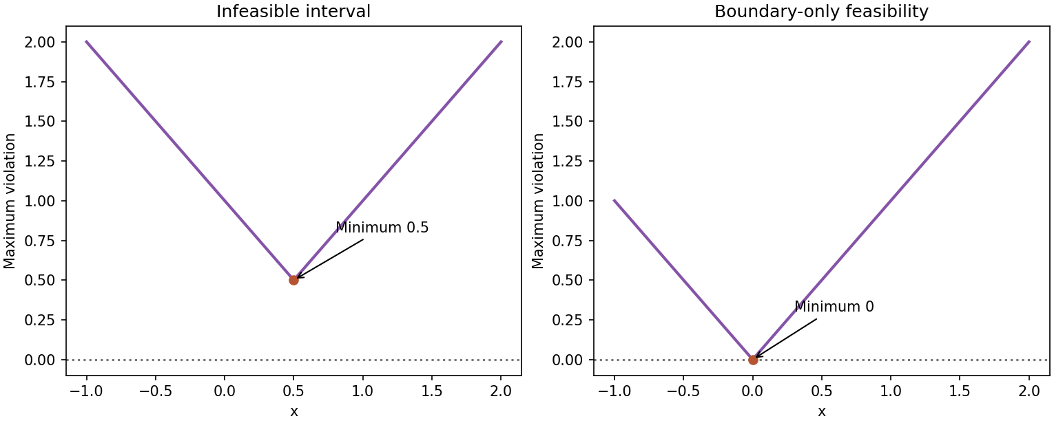
For the boundary-only system and , the only feasible point is zero. Eliminate the forced variable or represent the condition as an equality. Merely nudging the starting point fails because one inequality becomes violated whichever direction you move. The relevant interior is the relative interior after the forced equality is accounted for.
Phase I also depends on the domains of the . Relaxing their inequality values does not automatically make logarithms, matrix inverses or other expressions defined. Initialize inside the function domains or choose an appropriate reformulation. Inspect domain feasibility separately from the affine and inequality residuals.
Phase I has normalized dual prices
The maximum-violation formulation connects initialization to dual certificates. Attach multipliers to and multiplier to . Its Lagrangian is
Here are Phase I variables, its multipliers, and the original restriction data. Since is unrestricted, its infimum is finite only when . The inequality prices therefore form normalized nonnegative weights. A finite lower bound on the remaining weighted function bounds the largest original violation [1, Section 11.4].
For and , choose . Their weighted sum is exactly for every . Thus the Phase I optimum is at least ; choosing attains it. This supplies matching primal and dual values, proving that the original inequalities are infeasible.
For the boundary-only pair , , the same normalized sum is zero. The feasible Phase I point matches it, but no negative is possible. Zero violation can therefore prove ordinary feasibility without providing the strict interior needed by a logarithmic barrier. Eliminating the forced equality is the appropriate next modeling step.
7. Primal–dual steps and reliable stopping
A primal–dual method works directly with approximate optimality equations rather than completely solving each separate barrier problem. It maintains positive inequality multipliers and positive slacks, then solves a linearized system to reduce stationarity, feasibility and complementarity errors together.
Write the slack of inequality as and its multiplier as . For the original problem, the residuals include
Here is the stationarity residual, is the equality residual, and is the sum of complementarity products. The functions, matrix, multipliers and slacks have been defined above. For affine inequalities, separate slack equations can be included explicitly; nonlinear formulations may represent them through .
A small with a large feasibility residual is not a valid approximate solution. Nor does a small gradient in unconstrained coordinates establish constrained optimality. Require all relevant residuals, multiplier signs and domain conditions to pass. When the multipliers and primal point are feasible and stationarity holds, the complementarity sum corresponds to the duality gap; otherwise that interpretation needs qualification.
A fraction-to-boundary line search limits the step so the slacks and multipliers remain positive. It is a numerical safeguard for the algorithm’s domain, not a separate solution constraint. An infeasible-start method can initially violate affine equalities while still respecting the interior conditions needed by its formulas. Its merit function must reduce residuals, rather than simply evaluate the original objective at an infeasible point.
Sparse linear algebra often dominates the solve. The pattern of nonzero entries determines factorization fill, memory use and whether reuse is possible. A small iteration count can coexist with expensive iterations. Record factorization time and peak memory alongside iteration count when comparing methods. A dense educational implementation hides these costs and should not be used to predict large-problem performance.
Check the solution in the original formulation after canonicalization. A solver may introduce auxiliary variables and cones, normalize data, or remove redundant rows. These operations help computation, but the final application needs original-unit constraints and an interpretable objective. Record solver status, residuals, tolerances, formulation version and any postprocessing that modifies the returned point.
Linearize the primal–dual equations
A primal–dual Newton step targets the optimality equations jointly. For a quadratic objective with , affine inequalities , and equalities , use positive slack vector and positive multiplier vector . Let be the objective’s linear coefficient and the equality multiplier.
Define , , and . With a chosen complementarity target , linearization gives
Here specify the affine inequality coefficients and bounds; specify the equalities; are stationarity, inequality-feasibility and equality-feasibility residuals; and is the complementarity target. The quantities are increments; , , and is an all-ones vector. The last row linearizes the products , dropping only the second-order increment products. Unlike a full barrier centering solve, one step simultaneously reduces feasibility, stationarity and complementarity errors [1, Section 11.7].
If an increment has a negative slack coordinate, positivity requires step length in that coordinate. Apply the same rule to negative multiplier increments, take the smallest permitted bound, and stay slightly inside it. This derives the fraction-to-boundary safeguard rather than treating it as an arbitrary clipping rule. A further residual-decrease test is still needed: preserving positivity alone does not guarantee convergence.
8. Interpret a certificate at the application boundary
An optimality certificate answers a mathematical question about a specified model. An application decision also depends on whether that model includes the right constraints, quantities and uncertainty. Keep these two checks separate in the final report: numerical correctness cannot repair an omitted requirement.
Suppose a resource-allocation model limits total power but overlooks a per-device limit. The solver can return a globally optimal, accurately certified allocation that one device cannot implement. Add the missing constraint and solve again; do not describe the earlier result as a solver failure. Conversely, if every required constraint is present but the returned point violates one beyond tolerance, the issue belongs to numerical acceptance or the solve itself.
Choose tolerances before seeing the answer. A temperature bound, a budget equality and a dimensionless probability constraint need different interpretations of error. Write the acceptable deviations in original units, then connect them to solver tolerances and scaling. If a downstream rounding operation changes the variables, recheck feasibility after rounding. A certificate for the unrounded vector does not automatically certify the displayed or implemented decision.
Dual multipliers can explain sensitivity when the assumptions from the duality chapter hold. A large multiplier on a tight constraint suggests that a small relaxation may strongly affect the objective locally. It is not a prediction for an arbitrary large change, especially when the active constraints change. Test a small perturbation, resolve the problem and compare the observed objective change with the local prediction.
Near-degenerate problems deserve careful interpretation. Several almost redundant constraints can produce poorly determined multipliers while the primal decision is quite stable. A solver’s multiplier variation may then overstate uncertainty in the decision itself. Examine both primal sensitivity and dual sensitivity, and avoid reporting a shadow price with more precision than the data and conditioning justify.
Warm starts also belong to this boundary. Yesterday’s solution may be near today’s optimum but violate today’s updated constraints. A feasible-start barrier method must first find a new interior point. A primal–dual or homogeneous-embedding solver may handle a different initialization strategy. Pass a warm start only through a method that supports its feasibility state; do not clip variables independently when clipping can break coupled equalities.
A useful result bundle includes the formulation and data versions, original objective, primal variables, relevant multipliers, maximum original-unit violations, a gap or lower bound when valid, and the termination status. Add the measured time and memory if performance matters. This bundle lets another reader distinguish a trustworthy approximate optimum, an infeasibility certificate, an unresolved numerical outcome and a model that needs revision.
Modern view
Interior-point theory remains useful while current solvers make different choices about precision, memory and hardware. The following readings provide an algorithmic taxonomy and verified modern evidence through October 4, 2026.
Bubeck’s monograph [2] organizes convex optimization around oracle information, geometry and structure, covering first-order, structural and interior-point approaches. Its useful comparison is the cost of an iteration together with the guarantees attached to the oracle and assumptions. Our synthesis is to choose a method by the operations the problem makes cheap: matrix–vector products, projections, proximal maps or factorizations.
Parikh and Boyd’s proximal survey [3] maps nonsmooth, constrained and distributed algorithms through small convex subproblems. It complements the barrier viewpoint: a projection or proximal operation can enforce a constraint without representing its interior through logarithms. These operations can be inexpensive or costly depending on the set. A problem’s mathematical convexity does not determine which operation is affordable.
Goulart and Chen’s 2026 Clarabel paper [4] describes an interior-point solver for conic problems with quadratic objectives, using a homogeneous embedding and supporting several cone types. It connects textbook ideas to software that also addresses infeasibility and computational structure. Its comparisons apply to the tested problem sets and solver configurations; they do not establish one universal winner for every convex model.
Applegate et al.’s PDLP manuscript [5], first posted in 2025 and revised in 2026, develops a practical first-order approach to large-scale linear programming. It adds techniques such as preprocessing, scaling and adaptive behavior around matrix–vector operations. It is a preprint, and its performance claims are empirical for the reported workloads. The comparison with interior-point methods should include requested accuracy, memory budget and original-unit residuals.
| Solver family | Expensive operation | Typical structural question | What to verify |
|---|---|---|---|
| Equality-constrained Newton | KKT linear solve | can sparsity and factorization be reused? | feasibility and stationarity |
| Barrier/interior-point | changing curvature and constrained solve | is there an appropriate interior and cone representation? | domains, residuals, gap or certificates |
| Projection/proximal | projection or proximal subproblem | is the constraint or nonsmooth term simple to process? | iterate residual and feasible output |
| Large-scale first-order LP | matrix–vector products | does memory or factorization dominate the alternative? | scaled and original residuals at target accuracy |
The current methodological lesson is broader than a preference for first- or second-order methods. Formulation, preprocessing, scaling, linear algebra and stopping policy are part of the algorithm’s practical behavior. Comparing only the named update equation leaves out much of the system that determines reliability.
Open questions include accurate certificates for poorly scaled models, robustness when the feasible region is nearly lower-dimensional, memory limits in large factorizations and effective warm starts across changing constraints. A learned prediction can offer an initial point, but it still requires a feasibility and optimality check. Approximate solutions are useful when their errors are measured in the quantities the application can tolerate.
For a solver experiment, construct a family with one varying property: condition number, number of active constraints, sparsity or requested tolerance. Keep the mathematical optimum or an independently checked bound where possible. Report failures and inaccurate statuses alongside timings. Such a controlled family teaches more than a single successful solve with default settings.
Key takeaways
- Equality-constrained Newton steps remain in the nullspace of the equality matrix.
- The KKT matrix is generally indefinite even for a convex objective.
- A logarithmic barrier requires strict feasibility in the relevant domain.
- Exactly centered points yield a dual construction with gap under the stated assumptions.
- Numerical iterates need actual feasibility, stationarity and complementarity checks.
- Boundary-only feasibility differs from infeasibility; Phase I needs a certificate to distinguish them reliably.
- Compare solver cost, precision and memory in the original problem’s units.
Exercises
- Constrained curvature. Construct a positive-semidefinite quadratic whose full Hessian is singular but whose objective has a unique minimizer on an affine equality set.
Hint
Let a zero-curvature direction be excluded by the equality. Check positive curvature only along nonzero vectors satisfying the homogeneous equality.
- Equality scaling. Multiply the quadratic example’s equality by 1000. Compare the solution, multiplier and residual scales. Explain which quantities should remain invariant.
Hint
The feasible set is unchanged. The equality multiplier scales inversely, and raw residuals scale with the row. Verify stationarity in both representations.
- Duplicate barriers. Duplicate the upper-bound inequality in the scalar example. Compare the finite- central path and the count used in the theoretical gap.
Hint
The feasible set is identical, but the upper-bound logarithm appears twice. There are now three scalar barrier contributions.
- Initialization. Start the scalar barrier solver at zero and explain the failure. Give a principled repair for this problem and for a variable forced to zero by equalities.
Hint
A free nonnegative variable can begin strictly positive. A forced zero variable needs elimination or a suitable equality representation, rather than a numerical nudge.
- Infeasibility certificate. Generalize the contradictory interval to and with . Derive its minimum maximum violation and nonnegative certificate.
Hint
Balance the two violations at the midpoint. Equal weights cancel the variable and leave a negative right-hand-side sum.
- Stopping policy. A solver reports tiny complementarity but a nonzero equality residual. Write the additional checks needed before accepting its output, and explain why an objective-only report is insufficient.
Hint
Include original-unit equality and inequality residuals, domain checks, multiplier signs, stationarity and a valid lower bound when available.
References
- S. Boyd and L. Vandenberghe, Convex Optimization, Cambridge University Press, 2004, Chapters 10–11. Book and official PDF
- S. Bubeck, “Convex Optimization: Algorithms and Complexity,” Foundations and Trends in Machine Learning, 2015. Monograph
- N. Parikh and S. Boyd, “Proximal Algorithms,” Foundations and Trends in Optimization, 2014. Author page and article
- P. J. Goulart and Y. Chen, “Clarabel: An Interior-Point Solver for Conic Programs with Quadratic Objectives,” Mathematical Programming Computation, 2026. Published paper · Author manuscript
- D. Applegate, M. Díaz, O. Hinder, H. Lu, M. Lubin, B. O’Donoghue and W. Schudy, “PDLP: A Practical First-Order Method for Large-Scale Linear Programming,” arXiv preprint, 2025, revised 2026. Paper
Check your understanding
This tutorial has 6 exercises. Can you solve them without opening the hints?
Go to the exercises ↑Next OPT 08 · Geometric Applications, Splitting and Modern Methods · 22 min